May 4, 1988 - 1,5132. (. 18. ) RELATIVE. AZINUTH. _IN. NO,. 1. Z. 3. 4. 5. 6. 7. 8. ANuLEiOEG.) 0-9. 9-30. 30-bO. 60-_0. qC-1ZO. 120-150. 150-171. 171-180.
NASA Reference Publication 1184 1988
Angular Radiation for Earth-Atmosphere
Volume
ImShortwave
j. T. Suttles, P. Minnis,
and
Research
Hampton,
Hampton,
B. A. Wielicki
Center
Virginia
I. J. Walker Planning
Radiation
R. N. Green, G. L. Smith,
W. F. Staylor, Langley
Models System
and
Research
D. F. Young Corporation
Virginia
V. R. Taylor and L. L. Stowe NOAA National Environmental Satellite, Data,
and Information
Washington,
National Aeronautics and Space Administration Scientific and Technical Information Division
D.C.
Service
i | i
] 1
|
!
J | !
|
! J i =
!
|
Contents Summary
..................................
Introduction Symbols
.................................
Shortwave
and Angular
Directional Satellite
1
Grid
Model Parameters
Bidirectional
GOES
Parameters Parameters
Data
Nimbus
Sets
Data
Bidirectional Directional Overcast Results
3
...........................
3
...........................
4 4
.......................
5
...........................
5
..............................
Models Models
6
............................
6
.............................
7
.............................
8
Cloud Models
...........................
8
...................................
Bidirectional Directional
Models Models
8
.............................
9
.............................
10
Remarks
References
..................................
Appendix A--Application Bidirectional Models B
8
............................
Concluding
Figures
2
..........................
Processing
Processing
Models
Mixed-Scene
.........................
..............................
7 ERB Data
Model Development
Tables
1
...................................
Scene Types
Appendix
1
Equations
10
of Helmholtz ..................... for Mixed-Scene
Reciprocity
Principle
....... Properties
................
....................................
12 13 14
...................................
PRECEDING
to
19
PAGE
BLANK
NOT
III
I_LMED
:1 I!
Summary This document presents the shortwave angular radiation models that are required for analysis of satellite measurements of Earth radiation, such as those from the Earth Radiation Budget Experiment (ERBE). The models consist of both bidirectional and directional parameters. The bidirectional parameters are anisotropic function, standard deviation of mean radiance, and shortwave-longwave radiance correlation coefficient. The directional parameters are mean albedo as a function of Sun zenith angle and mean albedo normalized to overhead Sun. Derivation of these models from the Nimbus 7 ERB (Earth Radiation Budget) and Geostationary Operational Environmental Satellite (GOES) data sets is described. Tabulated values and computer-generated plots are included for the bidirectional and directional models. Introduction Analysis of satellite measurements for determination of the Earth's radiation budget requires information about the angular characteristics of radiation that is reflected (shortwave) 1 and emitted (longwave) 1 from the Earth-atmosphere system (Smith et al. 1986). The angular characteristics can be defined by models which express, for an imaginary surface element at the top of the atmosphere, the exiting radiance for each direction out to space as a function of the total hemispheric flux leaving the element. In principle, a radiance measurement at a single angle can then be converted into an inferred hemispheric flux. For successful application of the angular models, it is necessary to classify the Earth observations into a set of scenes (e.g., ocean, land, snow, and clouds) and to have a complete set of angular models for each scene class. Past investigations of Earth radiation budget from satellite measurements have varied considerably in the approach to angular models for reflected radiation. To analyze the Nimbus 3 measurements, Raschke et al. (1973) used three scenes (ocean, snow, and a cloud-land combination) and "gross-empiriear' models derived from a variety of sources including aircraft, balloons, and early satellite data. The scene identification was a static process, since the scene type for a given measurement location was determined a priori. Because of the lack of well-defined angular models, Gruber (1977) assumed isotropy for all shortwave observations while analyzing the National Oceanic and Atmospheric Adminstration (NOAA) I Reflected spectral marily
region
radiation (0 5#m),
in the longwave
occurs and region
primarily emitted (> 5 #m).
in radiation
the
Scanning Radiometer (SR) data. The isotropy assumption obviated the need for scene identification and detailed models; however, accuracy of the results was reduced considerably. For the Nimbus 7 Earth Radiation Budget (ERB) measurements, Jacobowitz et al. (1984) used four scenes (ocean, land, snowice combination, and cloud); a threshold method based on climatological values of reflected and emitted fluxes for cloud identification; and detailed angular models for each scene. The angular models for this analysis were derived by Taylor and Stowe (1984) from the ERB scanner observations. The ERB data processing was the first attempt to use a dynamic cloud-identification procedure for radiation budget analysis. The recent Earth Radiation Budget Experiment (ERBE) described by Barkstrom and Smith (1986) has a complex system of inversion algorithms which include angular radiation models. The ERBE inversion algorithms (Smith et al. 1986) use a set of 12 scenes, a Maximum Likelihood Estimation (MLE) scene identification method, and a comprehensive set of angular models. Because of the special requirements of the MLE method, statistical parameters are required as part of the angular model data set (Smith et al. 1986). The purpose of this report is to describe and present the shortwave angular models and associated statistical quantities that have been developed for the ERBE inversion algorithms. This report is Volume I of a set of two documents; Volume II describes the longwave models developed for the ERBE analysis. The shortwave models include bidirectional and directional parameters and were derived from existing Nimbus 7 ERB and Geostationary Operational Environmental Satellite (GOES) measurements and from theoretical relations. Bidirectional parameters are: anisotropic function, standard deviation of mean radiance, and shortwave-longwave correlation coefficient. Directional parameters are: mean albedo as a function of Sun zenith angle and mean albedo normalized to the overhead Sun value. A brief description of the model characteristics and derivation is presented. Tabulated values and computer-generated plots of the models are also included.
Symbols A
albedo
Ai
average albedo for ith solarzenith-angle bin
a,b
known values used in interpolation
shortwave occurs
pri-
coefficient
Cjk
in normalization
equation for anisotropic factors for angle bin with jth viewingzenith-angle and kth relativeazimuth-angle ranges COVAR(sw,
lw)
covariance and
E0
between
longwave
Earth
GOES
Geostationary Environmental
L
radiance,
L'
normalized
of viewing angle
it0
cosine
of solar
p
correlation
a
Budget Operational Satellite
M
radiation
flux,
Mi
average
radiation
W/m
flux
for ith
bin,
W/m
solar-zenith-angle number
2
2
shortwave anisotropic (defined by eq. (2))
function
average shortwave anisotropic factor for angle bin having ith solar-zenith-angle, jth viewingzenith-angle, and kth relativeazimuth-angle ranges r
Earth-Sun
ro
mean
$C, 0
unknown equation
distance,
Earth-Sun
azimuth
angle,
CR
relative fig. 1)
azimuth
and
Oo
solar
:
angle,
deg
(see
superscripts:
J
index bin
for viewing-zenith-angle
k
index bin
for relative-azimuth-angle
L
land
scene
bin
type
lw
longwave
m
index for a given an angle bin
mix
value for mix and 50-percent
n
index
for colatitude
0
ocean
scene
q
index
for seasons
r
reflected
8w
shortwave
albedo
function
zenith
observation
in
of 50-percent land
ocean
zenith
angle,
deg
deg (see
km
and
includes vegetated snow scene includes scene Data
for
Angular
bin
type
average
value.
Grid
and nonvegetated snow and ice.
types, and the There are twelve
types: nine basic types and three mixed types. for the land-ocean mixed scenes are derived
from values for the basic types as described in the section entitled "Mixed-Scene Models." Four levels
(see
fig.
Types
denotes
angle
The scene types selected for the ERBE data analysis (Smith et al. 1986) are used in this work. These scene types were defined on the basis of broad categories oi%]imat0iogically important surface and cloud features and are given in table 1. The desert scene
bin
angle,
a symbol
1)
of cloud coverage are included: clear sky (0 to 5 percent), partly cloudy (5 to 50 percent), mostly cloudy (50 to 95 percent), and overcast (95 to 100 percent).
2
_--
deg
for solar-zenith-angle
Scene
in interpolation
solar-zenith-angle
viewing fig. 1)
of radiance,
index
A bar over
km
distance,
values
normalized ith
deviation
radiance
of observations
number of observations for angle bin having ith solar-zenith-angle, jth viewing-zenith-angle, and kth relative-azimuth-angle ranges R
between
i
W/(m2-sr)
average radiance for angle bin having ith solar-zenith-angle, jth viewing-zenith-angle, and kth relative-azimuth-angle ranges, W/(m2-sr)
angle
longwave
¢
eq. (13)) Lijk
and
standard
Subscripts
(see
zenith
satellite)
W/(m2-sr)
W/m 2 (value distance)
radiance
(e.g.,
coefficient
shortwave
radiance
Radiation
cosine zenith
shortwave
solar constant, 1376 for mean Earth-Sun
ERB
#
=
11
The surface type at a given location on the Earth can be determined a priori by reference to a geographic map or atlas. The presence of a cloudy scene must be determined as part of the data processing using a scene identification technique. Note that a scene identification procedure must be applied during both the development and application stages for the angular models. Because of differences in measurements available in the two stages, the scene identification methods for development and application, in general, are not the same. The shortwave models in this report are defined according to the angular coordinate system shown in figure 1. The principal plane is the plane containing the ray from the Sun to the target area and the zenith ray that is normal to the target area. For an exiting ray (e.g., to a satellite), the relative azimuth angle CR is measured from the principal plane on the side away from the Sun. Thus, forward reflecting corresponds to CR = 0°, and backward reflecting corresponds to CR = 180°. To describe the angular variation of radiance, the angular coordinates are divided into ranges called "bins," and the model is represented by mean values for each bin. Table 2 gives the angular bin definitions for the solar zenith angle, viewing zenith angle, and relative azimuth angle. Symmetry about the principal plane is assumed for the azimuth angle. The illustration accompanying table 2 shows no bins for the first viewing-zenith-angle bin because, in fact, little variation exists. To derive a value for this socalled "cap bin," data for all azimuths are included in determining the average. However, as a practical matter for computer application, azimuthal bins are also provided for the first zenith bin to avoid indexing problems. This is accomplished by replicating the cap-bin value for all azimuths. The data presented in this report include this replication. Shortwave
Model
Parameters
Bidirectional
Parameters -a7
,76 2.6 -.34b
(!0) (10) (I0)
.76 Z.5 -.638
(I0) (10) (lb)
,73 2._ -,411
(i01 (I0) (10)
.b7 _o7 -.369
(i0) (I0} (IC)
,6E 2._ -,305
liD) liD) (iC)
,68 _,9 -,356
(I0) (I0) (i0]
,70 Z,_ -.600
410} (I0] (I0)
,72 _o_ -.458
(101 (I01 (10)
_7-39
.85 2.7 -,239
(_) (q) ( 9)
.e2 3.0 -.337
[Ib) (_u) [i0)
.76 _.9 -,668
(I0) (Iu) (101
.72 2,5 -._lZ
(i0) (i01 (10}
.7_ a.E -._7_
(iO) (iO) (10)
,74 Z,8 -.368
(IO) (lO) (lO)
,76 1,3 -,_T6
(I0) (lO) (lO)
.83 _.7 -,331
( 9) ( _) ( q)
_9-5_
*.12 3.6 -,26b
(I0) (/0) (i0)
l. U5 3.0 -,231
(_u) (ib) (lu)
• 91 3.1
5
_l-b3
1,61 5.9 -.17_
(i0) i/U} [iO)
1.42 5.0 -,036
(i_) (I0) {iu)
o
_J-75
3.i0 ZC,2 -,05v
(i01 (I0) (I0)
2.3E 11.6 -.013
7
f_-90
3.07 _7.8
3
5._0 29.8 -.028
2.00
(g) { q) (
9]
-.173
(10) (10)
.79 2.5
(10) (10)
-.28o
(lO)
-.323
(1C)
-._05
(10)
-,196
(lO)
-.38Z
(lO)
-.225
(lO)
l.i_ 3.b 1,058
(I0) (10) (10)
.82 _.7 1.1Z5
(I0} (10} (10]
,8! Z._ m'_04
(I0) (10) (1O)
._ 3.Z --'333
(tO) (10) (10)
1.01 2.6 --'368
(lOl (10) (10)
.qq 2.5 --.Zk8
(I0) (101 (101
(i_) (11} (i_)
1.o6 6.1 -.17_
(iO) (10) (10)
.Qb 3.7 -,227
(i0} (10) (10)
.q_ 3.C -.kl_
(iO) (10) (lO)
l.lb 3.5 -._0_
(I0) (lO) (lO)
1.28 3,Z -,314
(II) (11) (11)
l,ZP 3.7 -.18_
(i01 (10) (lOI
(10) (lu)
Z.3Z 8.8 -.ZZ9
(10) (10) (10)
1.50 5,4 -.19_
(5) ( 5] ( 5)
1.35 6,3 -.Z6_
(5) ( 5) ( 5)
1.48 4.1 -.015
(q) ( q) ( _)
1.Sq 3,4 -.Z85
(10) (10) (lO)
1.b7 3,1 -,_23
(9) ( 9) ( q)
(lul
-
/
,77 2.5
2.00
(lO) (101
,T8 3.1
(lO) (1O)
.83 2.3
(10) (lOI
.86 z.q
(lO) (1CI
--
1.75
1.75
1.50 1.50
0 0 ,( 1.25 U.
_b1.25
/1t
1.00
0
.75
I
0 1.00 0 C_ .75
AZIMUTH
AZIMUTH
BIN 1 2 3 4
.50
.2
I I 1 I I I I I I 0
10
20
30
40
VIEWING ZENITH
50
80
ANOLE(
(j)
70
80
.SO
.25
--
I I I I I I I I 1 0
10
20
30
40
VIEWING ZENITH
DEO )
Solar-zenith-angle Figure
5 6 7 8
--
0
90
BIN
Z
50
60
ANGLE(
70
80
gO
DEG )
bin 10, 84.26 ° to 90.00 °. 9.
Concluded.
51
SCENE DATA
SUN MEAN NORMALIZED
TYPE 1 Z 3 ( )
ZENITH ALBEDO ALBEDO
RELATIVE I C-q
BIN NO, ANGLe(DE6,) VI_wIN_ ZEhLT_ bin NO, ANbLE(bE_,) 1 0-15
Z q-30
1.o7 23,_ -.lOJ
(1l) (111 (11)
Z
1_-27
1._b 23.8 -.DZo
(i0) (1_) (10)
3
17-30
.q_ 23.8 -.Oeb
(101 (10) (10)
_9-_1
1.07 23.0 -.lu_
3 30-60
: : s
,C .2369 1.0C00
25.8 ( 14 ( 16
SW RADEANCES(WINee21SR) SW RADIANCES
) )
AZIMUTH
4 60-_C
5 QC-120
6 120-150
7 150-171
B 171-180
(11) (111 (11)
1.07 23.0 -.10G
(11) (11) (11)
1.07 23.0 -.100
(111 (11) (111
1.07 23.C -.10C
(11) (111 ill)
1.07 13.0 -.I00
(11} (11) (111
1.07 23.0 -.100
(11) (11) (11)
1.07 23.0 -.100
(111 (11) (11)
._g 24.1 .004
(11) ill) (lid
1.03 14._ -.OlO
ill) (lid (11)
1.04 24.0 -.081
(11) (11) (11)
1.0_ 23.C -.09_
(11) (11) (11)
1.08 22.7 -.194
(11) (lid (11)
1.09 21.6 -.227
(11) (Ill (11)
1.12 22.0 -.252
(11) (11) (11)
.98 2_.2 -.Oe?
{11) (1_) (i_]
1.01 Z4.2 -.0_5
(11) (11) (111
1.01 2_.1 -.130
(11) (11) (111
1.O_ 23.4 -.176
(11) (11) (11)
1.05 22.4 -.229
(11) (111 (Ii}
1.09 22.3 -.229
ill) (11) i11)
1.08 21.6 -.292
(10) (101 (101
._2
(1C)
(111
.q_
(11)
1.00
(11)
1.0_
(111
1.02
(11)
1.05
(11)
1.03
(11)
2_.t .04_
(101 (101
24.e -.103
(11) (111
24.7 .01_
(11) (11)
24.0 -.O4Q
(11) (11)
23._ -.151
(11) (11}
22.3 -,214
(11) (111
22.8 -.188
(111 (11)
22.4 -.136
(11) (11)
_1-b3
._1 23.u -.o_e
(10) (13) (10)
._3 24._ -.O_
(111 (1.) (11)
.ql _.o .031
(lid (111 (11)
.qB 24.0 -.064
(10) (10) (10)
.94 22.E -.14_
(lid (I1) (11)
1.01 22.1 -.149
(lid (111 (111
1.02 22.4 -.190
(Ill (11) (111
1.01 22.3 -.153
(11) (11) (11)
b
0_-7_
._ Z_._ -.0_2
(10) (iu) (101
.93 2_.1 -.142
(111 (11) (111
.91 23.5 -.Oq_
(11) 411) (11)
.94 2_.4 -,161
(11) (11) (11)
.97 22._ -.2_(
(11) (11) (111
1.00 20.9 -.148
(11) (111 (11)
.98 21.5 -.110
(11) (111 (11)
.99 21,3 -.1_9
(11) (111 (11)
7
75-_
._ _.7 -.153
(lO) (10) (10)
.q_
._3 21.9 -.13_
(10) (1_) (101
.go 21._ -.0_7
(11)
,@7
(Ill (11)
(10)
18.8 -.093
2.00
1.75
--
1.75
l
1.25
(lO) (10)
.98 18.b -.214
(101 (10) (10)
.96 18.2 -.094
(11)
.98
(10)
(11) (11)
20.0 -.242
(10) (10)
"50
--
1.25 I
--
IJ.
L_
0 _. 1.00 0 Q::
r..) _. 1,00 0 n,_)
.75
AZIMUTH
(,rl
z
AZIMUTH
_m
BIN I
50
.7S
l
50
"
I
n," 0 I-C)
(101
lq.C -.27_
l
--
F-0
.9E
(lO) (10)
2.00
1
s CLEJR DESERT - SW JNISOTROPIC FACTOR - STANDARD DEVIATION Of - CORRELATION OF LW AND - DATJ SOURCE
_
BIN 5 6 7 8
.SO
.25
25
I I I I I I I I I 0
I0 20 :30 40 VIEWING ZENITH
50 60 ANGLE(
70 DEO
80 )
gO
(a) Solar-zenith-angle Figure
10. Bidirectional
model
for clear over desert.
0 I I I I I I I I I 0
10 20 30 40 VIEWING ZENITH
50 60 ANGLE(
70 DEO
ISO )
bin 1, 0° to 25.84 °. (See table 5 for explanation
52
i
of data
sources.)
9O
ORIGINAL OF
PAGE
POOR
SCEHE DATA
IS
TYPE 1 2 3 ( )
QUALITY SU_
ZENITH
!
2_,E
ALBEDO ALBEO0
! ;
,2388 1.0080
VLtWLN_
3 30-60
q-3C
0-q
CLEAR DESERT Sw $NISOTRDPZC FACTOR STANDARD DEVIATIDN OF CORFELATIDN OF LW AND OATA SOUPCE
MEAN NUE_ALIZED
RELATIVE
ANGLf(DEG.)
I -
-
SW RAOIANCES(WIHee21SR) SW RADIANCES
3b.% [ (
1_ 1_
) )
AZIMUTH
_ 60-%0
5 9C-120
6 120-1_0
T 150-171
e 1Tl-180
_LNITH _-15
.gV 24,4 •ogG
(11) (11) (11)
,g9 2_.& .U9¢
(11) (1_) (11)
,Qg 2_._ ,09G
(11) (11) (11)
,g9 2..4 ,090
(11) (11) (11)
,9; Zk.; ,OgC
Z
i_-Z7
.9_ ZS.O -.Or7
(iv) (10) (i_)
.$g 24,o ,155
(lu) (LO) (L0)
,99 29,6 ,008
(11) (11) (11)
,97 2;,3 -,003
(11) (11) (11)
1,01 (11) 25,((11) ,01; (11)
3
_1-3_
.99 26._ -.OZ_
(10) (10) (I0)
.Q5 26.9 -.0;4
(1v) (LO) (1_)
.q2 2_.7 -.037
(10) (10) (10)
,_5 22.3 ,102
(10) (10) (10)
,gE 22,2 -,06_
39-_1
.8_ _._ ,0_
(IO) (lOJ (10)
._9 27.1 -.01_
(11) (_1) (11)
.87 24._ .0_
(10) (10) (10)
,_7 25,0 -,C89
(10) (10) (10)
1,01 2_,_ -,11¢
_1-o3
._ l_._ • O1_
(10) (I_) (iv)
._C 26.7 -.0_6
(_0) (10) (_O)
,go 25,7 -.037
(1C) (1C)
1.O1 27.2
(10) (10)
,g_ Z3,2
(1C) (10)
1,10 26.0
(10) (10)
(10)
,01]
(10)
,058
(10)
-,022
(10) (10) (10)
1,03 2_,_ -,103
(10) (10) (10)
(5) (5) (_)
1,05 23.7 -,0_
(6) (6) (6)
(10}
-.102
6
o5-7)
1,00 Z7._ -.1_
(iO) (10) (10)
._2 24.2 -,I2_
(11) (1_) (11)
,8_ 23.8 -.023
(11) (11) (11)
,_3 26._ .Z_3
(10) (10) (10)
.q_ 21._ -.00_
7
7_-90
1.11 lo,_ -,13_
( ( (
1.C2 2_.9 -.2_1
(lu) (i0) (10)
.9_ 2_.2 -,Obb
(10) (10) (10)
._9 Z5.6 .132
(8) (B) (B)
,_ 22,£ .034
9) 9) 9)
2.00
2.00
1.75
1.75
rv" 1.50 O Ft.) -90
2,Ol _3,_ .oco
(12) (13) (O)
1,99 t2,9 .000
(12) (13} (_)
1,71 10,0 .OoC
(123 (13) (D)
1,41 9,5 .000
(123 (13) O)
1.4_ 8,_ • OOf
(1E} 413) (C)
1.79 I0.0 .000
(12} (13) (O)
2,10 10.6 .000
(123 (13) O)
2.1q IO,0 .000
(12} (13) O)
7
.q_
//
2.00
2.00 1.75
--
1.25
/f
1.75
r_ 1.50 O I--
S!J
--
) (2)
1,63 q.7
(2) (2)
1,42 7.2
(2) (2)
1.65 6.3
(2) (2)
-,DOg
(2)
.065
(
( 2} (2)
1.0_ 8.1
,6d 4,6 -.041
(2) ( 2}
,84 6,8
2)
-,Iii l.
2,58 I_.8
(2) (2)
(2) (2) (2)
-,OBg
(2)
,.oo_ ///
-.03!
2}
1,94 8.2
(2) ( 2}
2._3 12.e
(2) t 2)
.005
(2)
,192
(
i 2"00
F
1.75
F
2!
•
1.75
(Z: 1.50
//
-
--
/
//
C)
/ 1 25
0
/_//i/
II
///
¢D
./Y 1#// /
_O100
_.._ _ J
(/I "