angular reconstitution in three-dimensional electron microscopy

Scanning Microscopy Vol. 11, 1997 (Pages 179-193) Scanning Microscopy International, Chicago Angular (AMF reconstruction O’Hare), ILin60666 3D electron USA microscopy

0891-7035/97$5.00+.25

ANGULAR RECONSTITUTION IN THREE-DIMENSIONAL ELECTRON MICROSCOPY: PRACTICAL AND TECHNICAL ASPECTS M. Schatz1,3,*, E.V. Orlova2,4, P. Dube3,4, H. Stark2,4, F. Zemlin2 and M. van Heel2,4 1

Image Science Software GmbH, Berlin, 2Fritz-Haber-Institut der Max Planck Gesellschaft, Berlin, 3 Max-Planck-Institut für Molekulare Genetik, Berlin, Germany 4 Department of Biochemistry, Imperial College of Science, Medicine and Technology, London, UK Abstract

Introduction

Cryo-electron microscopy in combination with the angular reconstitution technique has become an important and rapid technique for analyzing the three-dimensional (3D) structure of individual, non-crystallized biological macromolecules. Behind this technique is the idea that a 3D structure can be calculated based on a very large number of images of individual molecules randomly oriented within a homogeneous matrix. The approach has great practical and theoretical advantages over earlier techniques which require tilting of the specimen holder in the electron microscope. We want to elaborate on some of the specific details of our procedures. For example, alignments are used to remove the “in-plane” positional x- and y-shifts, as well as the inplane rotations of the molecules. Automatic classification procedures are subsequently used to find the different characteristic views of the molecules due to “out-of-plane” rotations of the molecules. The characteristic views are assigned Euler angles by the angular reconstitution technique using sinograms and sinogram correlation functions under the boundary conditions dictated by the pointgroup symmetry of the structure. Three-dimensional reconstructions can thus be calculated; and once a preliminary reconstruction is available, iterative refinements are applied to further improve the quality of the results.

The principles of the angular reconstitution approach have been published in the late eighties (van Heel, 1987; Goncharov and Gelfand, 1988). In an accompanying paper we place this technique in a historical perspective and compare the approach to other related techniques. In this paper we concentrate exclusively on the practical aspects of our own procedures. Although the methods were already published about ten years ago, the practical application of that technique to real electron microscopical data sets of biological macromolecules required further algorithmic improvements and the development of various iterative refinement procedures. The first full paper applying our angular reconstitution algorithms in low-dose electron cryomicroscopy on the structure of the closed state of the calcium-release channel appeared in January 1995 (Serysheva et al., 1995). The angular reconstitution approach aims at exploiting the random orientations that macromolecules can assume within a homogeneous embedding medium. When thousands of molecular projections in all possible orientations are available, that information can be integrated into a single three-dimensional (3D) structure calculated from these thousands of images. Since this approach does not require any (macroscopic) tilting of the specimen holder in the electron microscope with its attendant disadvantages (such as defocus gradients, changes in the specimen/ microscope between tilts), it has great practical and theoretical advantages over most earlier single particle techniques. The electron microscope (EM) produces almost perfect projection images of the molecules in a plane perpendicular to the beam, and thus the z-position of the molecules within the embedding medium is, to a first approximation, irrelevant. The molecules, however, then still have 5 degrees of freedom that need to be taken into account in order to calculate the 3D structure. First, the molecules may be located anywhere in the micrograph, and we thus need to determine their exact (x,y) positions. Moreover, at that (x,y) position, a molecule can have any orientation in terms of an “in-plane” rotation (we call this rotation the α -angle rotation). Reference-free and cross-correlation-based

Key Words: Angular reconstitution, Euler angles, sinograms, sinogram correlation functions, three-dimensional reconstruction, automatic classification, alignment, image processing, cryo-electron microscopy, structural biology.

*Address for correspondence: Michael Schatz Image Science Software GmbH Heilbronner Straße 10 D -10711 Berlin, Germany Telephone number: +49 30 - 8909 5326 FAX number: +49 30 - 8909 5321 E-mail: [email protected]

179

M. Schatz et al. alignment procedures are used in order to eliminate these three in-plane degrees of freedom (x, y, α). At this (x, y, α) position and orientation the molecule still has two further degrees of freedom of “out-ofplane” rotations, say, around the x-axis and around the yaxis. Actually, in an object-centered coordinate system, we normally describe the three rotational degrees of freedom (three “Euler angles”) of the molecules as a rotation “γγ” around the z-axis, followed by a rotation around the y-axis β”, which is then followed by the α rotation, again around “β the z-axis. Automatic classification procedures are used to find the different “characteristic views” (Van Heel and Stöffler-Meilicke, 1985) associated with these two out-ofplane rotational degrees of freedom (γγ, β). The characteristic views are then assigned Euler angles by the angular reconstitution technique per se in which sinograms and sinogram correlation functions are used, under the boundary conditions dictated by the pointgroup symmetry of the structure. Three-dimensional reconstructions can subsequently be calculated using a 3D reconstruction technique which correctly weighs the various characteristic views contributing to the 3D map. Once a (preliminary) 3D reconstruction is available, reprojections of the 3D map are used as references to realign the full data set by further multi-reference alignments. In this phase of the analysis, all Euler angle assignments are performed with respect to a small set of reprojections of the map, the socalled “anchor set”. All procedures are iterated until no further improvements of the various quality criteria are observed. The angular reconstitution technique has now evolved into a powerful and rapid technique for elucidating 3D structures of individual non-crystallized macromolecules (“single particles”) imaged in the cryo-EM, as has been illustrated in a number of studies of biological macromolecules recently published. Resolutions of up to 15Å have been obtained for symmetrical particles (Serysheva et al., 1995; Schatz et al., 1995; Tavares et al., 1995; Dube et al., 1995a,b; Orlova et al., 1996), but the technique may equally well be applied to asymmetric particles such as the 70S E. coli ribosome (Stark et al., 1995, 1997). The general philosophy of the method and its historical development are discussed in a separate paper in this issue (van Heel et al., 1997). Here we focus on the image processing protocols and on the various iterative refinement procedures used during a typical 3D analysis of a macromolecular complex. Note that all procedures discussed are implemented within the IMAGIC-5 image processing system (van Heel and Keegstra, 1981; van Heel et al., 1996).

most important aspects of (cryo-) electron microscopy. The actual electron microscopy is equally crucial for attaining high-resolution results on a good specimen. Indeed, now that 3D single-particle electron microscopy is approaching the 10Å resolution level, these microscopy-oriented issues are of central importance. Nevertheless, the starting point of our discussion here occurs after the good micrographs have been collected. It is important to maintain the good quality of the micrographs during the digitization process. A key issue in digitization is the numerical aperture (NA) of the optical system used for looking at the micrograph. This issue appears to have received too little attention in recent years which, in turn, appears to have caused some unnecessary problems in practical analyses. Microdensitometers, such as the Perkin Elmer (Norwalk, CT) PDS, are high-resolution scanning devices which are typically operated with a light-microscopical 5x or 7x objective lens with an NA of ~0.2. With such a diffraction-limited optical system, a resolution of ~2 µm (point-to-point resolution: Rayleigh criterion) may be achieved which allows one to comfortably digitize a micrograph using ~5x5 µm2 pixels (the limit being ~1x1 µm2, or twice the “Nyquist” frequency). Note that we here are looking only at the optical resolution issue: it is clear that at this level of resolution other factors such as the grain size of the emulsion, the mechanical stability of the set-up, and the flatness of the x-y table enter the equation. However, such high-resolution microdensitometers typically measure only one pixel at a time and scan the micrograph mechanically in both directions, a process which can lead to excessively long digitization times. The amount of data that we need to digitize for a single project can be ~100 micrographs. On a high-resolution microdensitometer it may already take a day to digitize a single micrograph to high resolution. These devices are thus simply not fast enough for our purpose. Much faster devices are available which digitize a micrograph in a few minutes by scanning a linear CCD (charge-coupled device) array over an image of the micrograph; this image is generated by a (to an approximation) diffraction-limited lens such as the APO-Rodagon D (Optische Werke G. Rodenstock, Munich, Germany). The Kodak “Eikonix” (Eastman Kodak, Rochester, NY) and the Image Science “EMiL” scanner (Image Science Software GmbH, Berlin, Germany) are typical examples of this family of densitometers. These devices, which use photographic lenses rather than light-microscopy objectives, can also give good results provided one uses the optical system wisely (and provided these devices are mechanically stable and do not suffer from vibrations). A high-quality optical lens like the APO-Rodagon D (similar lenses are manufactured by other lens manufactures such as Zeiss (Carl Zeiss, Oberkochen, Germany), or Nikon (Nikon Corp., Tokyo, Japan) may operate in the diffraction-limited regime for relative

Electron Microscopy and Densitometry Specimen preparation is undoubtedly one of the

180

Angular reconstruction in 3D electron microscopy apertures in the range of f:5.6-11. Assuming one uses such a good lens optimized for 1:1 imaging (“4F” configuration: the object plane is 2 focal distances F in front of the lens, the image is 2F behind the lens), then the numerical aperture for the 1:1 optical system may be estimated from the equation: NA = D/4F = 1/4f

Meilicke, 1985) (Fig. 1, row 1). We routinely band-pass filter to suppress disturbing very low and very high spatial frequencies (Fig. 2). In our experience, this filtering is a very important first step in all image analysis of biological macromolecules. The presence of strong low frequency components in the images (often associated with density ramps) may especially seriously disturb many aspects of the subsequent data processing. For example, alignment procedures using cross-correlation functions are very sensitive to the presence of disturbing low frequencies. The very high frequencies in the images may represent only unwanted noise and can thus also be suppressed. However, suppressing these frequencies is in practice less important than suppressing the very low frequencies; moreover, these very high spatial frequencies may also contain the essential highfrequency information one is seeking (see previous paragraph). The applied band-pass filter is the product of a wide Gaussian low-pass filter to cut away the very high spatial frequencies, and a narrow Gaussian high-pass filter to cut away the disturbing low frequencies. One may choose to leave in a fraction of the very low frequency components in the data (say, 0.001) in order to be able to restore these components in the images at a later stage. The parameters of the band-pass filter (Fig. 2) are chosen considering the overall size of the particle (the low-frequency cut-off) and the expected resolution in the data (high-frequency cutoff). During the first iterations of a 3D single-particle analysis it may first be necessary to suppress the high frequencies to find a rough, preliminary 3D model for the later refinement procedures, during which the high frequencies are reintroduced for obtaining high-resolution results. The filtering parameters may thus be adapted in the course of the processing. After suppressing unwanted frequency ranges, one then typically removes unwanted background by imposing a circular mask to the filtered images. The data within the mask is then normalized to zero average density and an arbitrary variance value of 100 (van Heel and StöfflerMeilicke, 1985). These pretreated images all reside in a single IMAGIC file (van Heel et al., 1996) and are used as the starting point for all subsequent alignments, which is discussed below.

(1)

In this equation D is the diameter of the lens, F its focal length, and f is the relative aperture F/D). Thus, at f:8 the numerical aperture of this system is NA≈0.03, and the diffraction limit will be around ~15 µm. The EMiL densitometer, for example, has 7x7 µm2 pixels in its CCD line, a sampling still appropriate for the optical resolution of this 1:1 setup. However, when the light level is too high, one might naturally tend to close the lens aperture to, say, f:22. At that relative aperture, however, the resolution of the imaging system - still assuming it to be diffraction-limited has dropped to ~40 µm and sampling with a pixel size smaller than 20 µm is useless. It is much better to reduce the light by, for example, decreasing the integration time of the CCD camera while keeping the lens aperture at, say, 5.6. Thus, as is demonstrated by this example, digitizing systems need to be used with (love and) understanding. A new generation of hybrid densitometers has recently emerged in which a high NA lens (NA ~0.2) guarantees high optical resolution, yet that lens images a large area of the micrograph, say, 512x512 pixels, onto a square cooled CCD chip which digitizes that extended area at once. Stepper motors driving the stage that hold the micrograph then allow the micrograph to move to the next square such that it is digitized checkerboard-wise (Schatz and van Heel, 1994). This hybrid densitometer thus combines the high resolution of the conventional pixel-by-pixel microdensitometers with the high speed of the linear CCD electronic scanners. In the long term, one may expect the photographic film to become superfluous with the advent of affordable, large-area CCD arrays to be used inside the microscope, or with improvements of the imaging plate technology to very high resolution. At present, the breakeven point between these novel technologies and the conventional photographic film that can store very large amounts of information has not yet been reached for this application.

Reference Free Alignment Pretreatment of the Molecular Images The raw pretreated images of individual biological proteins are excessively noisy and are difficult to appreciate visually. The first priority is thus to develop a feeling for the data, in particular to understand whether the data contains a wide range of characteristic views (a good preparation) or just a few preferred orientations (a bad preparation). This

Once the digitized micrographs are available in the computer, the individual particles may be selected interactively or by automatic techniques. For a number of reasons, the raw images of the individual macromolecules first need to be filtered and normalized (van Heel and Stöffler-

181

M. Schatz et al.

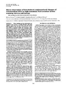
Figure 1. A summary of the image processing and 3D reconstruction of Lumbricus terrestris hemoglobin (at 30Å resolution). Row 1: Some original molecular images after band pass filtering and normalization (Fig. 2). These images are members of the corresponding class averages shown in the second row. Row 2: Some characteristic views (class averages) obtained by multi-reference alignment and multivariate statistical classification as described in the main text. Row 3: 3D surface representation of the reconstructed 3D volume in viewing directions corresponding to the Euler angle orientations of the images shown in rows 1 and 2. Row 4: The 3D structure of the Lumbricus terrestris hemoglobin molecule is reprojected in Euler directions assigned to the class averages (row 2).

“Double Auto Correlation Functions” (Schatz and van Heel, 1990) or “Double Self Correlation Functions” DACF/DSCF classification techniques (Schatz and van Heel, 1992). Our favorite reference-free alignment procedure is the alignment-by-classification technique (Dube et al., 1993). In this approach, the selected molecular images are first centered by translational alignment relative to the rotationally averaged total sum of all images in the set. Multivariate statistical classification procedures (see below) are then used to find similar images, in similar rotational orientations. An additional advantage of this procedure is the unbiased finding of symmetry properties of the molecule (Dube et al., 1993; van Heel et al., 1996). The class averages resulting from this procedure are then used as a first set of independent reference images for a multi-reference alignment (MRA) procedure (van Heel and Stöffler-Meilicke, 1985).

aspect of the data processing is particularly important when the first images of a new sample must be evaluated. Because of the very high noise level in the images, it is virtually impossible to judge the quality of the molecular images without first applying averaging procedures to improve the signal-to-noise ratio (SNR). To average images, however, it is necessary to align the molecular images and to sort them into homogeneous groups (“classes”) showing the same molecular view. Images within such homogeneous groups may be averaged into “characteristic views” (van Heel and Stöffler-Meilicke, 1985). Aligning a set of images with respect to a reference image using correlation function-based alignment procedures (Frank et al., 1981, Steinkilberg and Schramm, 1980; van Heel et al., 1992a), i.e., eliminating the “x, y, α” degrees of freedom, however, tends to bias that data set towards the reference image (Boekema et al., 1986) and thus is not a technique suitable for obtaining a first overview of the data. We have developed “reference-free” alignment techniques to avoid the reference bias problem which uses invariant

182

Angular reconstruction in 3D electron microscopy for more than a decade now and can be considered standard. MRA procedures are used in various phases of the iterative analysis, as will become clear below, and not only in the preparative phase we have just described. Automatic Multivariate Statistical Classification Multivariate statistical analysis (MSA) classification was introduced to electron microscopy some 15 years ago (van Heel and Frank, 1981) and is now an integral part of many image processing procedures. With the MSA techniques one considers images as a linear combination of the main eigenvectors (eigenimages) of the set, thus reducing the total amount of data and facilitating the interpretation. Although the eigenvector analysis was originally performed using the χ2-metric, we now prefer using the modulation metric (Borland and van Heel, 1990). This metric can deal with phase-contrast EM images which may have a zero average density, a situation which cannot be dealt with in strict correspondence analysis other than either by adding a constant or by thresholding the negative densities away. Strict correspondence analysis uses a χ2metric which is designed for positive data such as histogram data. In our standard pretreatments of the molecular images (see above) we cut away virtually all low frequency image components leading to images which essentially have a zero mean. Such images could not be used for the strict correspondence analysis χ2-metric. For high-resolution EM work the χ2-metric must now be considered obsolete. After the MSA eigenvector eigenvalue data compression, an automatic hierarchical ascendant classification in combination with a moving elements post-processor (van Heel, 1984, 1989; Borland and van Heel, 1990) operating on the compressed data is performed. A number of quality criteria are included in the classification procedures in order to, if necessary, eliminate poor images and classes from the processing. The images which have been assigned to a single class are then averaged and subsequently used as references for a new MRA / MSA classification iteration round. After a few iterations good class averages with improved signal-to-noise ratios can be obtained (Fig. 1, row 2). One of the quality criteria used as an indicator of convergence of the procedures is the internal resolution of the class averages estimated with the S-image (Saß et al., 1989) or the I-image (manuscript in preparation). The low noise levels obtained in the averages (high SNR values) are of great importance for an accurate determination of Euler angles (cf. Schatz et al., 1995).

Figure 2. Schematic diagram of the band-pass filter applied routinely to the data sets. A band-pass filter reduces the influence of irrelevant and often disturbing spatial frequencies. A double Gaussian filter is applied in Fourier space defined by three parameters: 1) a high frequency cutoff is associated with a low-pass Gaussian filter which will gradually cut off frequencies higher than that value, 2) a low frequency cut-off is associated with a high-pass Gaussian filter which gradually cuts off spatial lower than this value, and 3) a remaining low frequency transmission parameter allows one to leave a fraction of the lowfrequency components (say, 0.001) intact such that one can always restore these low-frequency components at a later stage by inverse filtering, without dividing by zero. The parameters displayed in this curve are chosen for illustration purposes only.

Multi-Reference Alignments β,γγ) projections of a For data sets in which different (β structure are mixed (the type of data sets needed for the angular reconstitution approach), we need many different reference images for performing a good align-ment of the molecules. It is normally impossible to achieve a good overall alignment of a mixed population of images using just a single reference image because a 3D structure projected into different directions normally yields very dissimilar projection images. Correlation-function based alignment procedures require the image to be aligned to resemble the reference image; after all, they need to “correlate”. In consequence a (large) number of projection images are required as reference images to align a mixed population of images. MRA (van Heel and Stöffler-Meilicke, 1985) have been in routine use

Euler Angle Assignment The class averages resulting from the above procedures are two-dimensional (2D) projections of a 3D structure

183

M. Schatz et al. in different projection directions. After having found a sufficiently large set of good, noise-free 2D projection images, we can reconstruct the 3D structure to high resolution (Klug and Crowther, 1972; van Heel and Harauz, 1986). Prerequisite for calculating a 3D reconstruction is that the orientational relationships between all projection images are known. These orientational relationships can be found with the angular reconstitution technique (van Heel, 1987; Goncharov and Gelfand, 1988; van Heel et al., 1992b; Farrow and Ottensmeyer, 1992; Radermacher, 1994). The technique is based on the common line projection theorem (van Heel, 1987) stating that any two 2D projections of a 3D object share at least one line projection. This common line projection theorem is the real-space equivalent of the Fourier space common line theorem (DeRosier and Klug, 1968). By searching for the common line projections, one can determine the spatial relationships between the set of projection images. To find the common line projection(s) between two 2D projection images, their sinograms (collection of all possible line projections of the 2D projection) are compared line-by-line in “sinogram correlation functions” (van Heel, 1987). At a position corresponding to a pair of shared line projections, the sinogram correlation function has a maximum. If the molecules exhibit a specific point-group symmetry, the sinogram correlation function shows a number of corresponding, symmetry-related peaks. Highly symmetric molecules such as icosahedral viruses or the worm hemoglobin (Schatz et al., 1995) are somewhat easier to process than asymmetric particles (Stark et al., 1995; 1997) because the redundancy of the symmetry-related peaks in the sinogram correlation functions lead to a fast convergence of the Euler angle assignments. The Euler angle determination is performed stepwise by including an increasing number of projection images into a set of images which have already been assigned Euler angle orientations. The search for the peak(s) is performed as a complete (“brute force”) search over all possible Eulerangle orientations corresponding to the full asymmetric triangle for the given point-group symmetry (Schatz et al., 1995; Serysheva et al., 1995). The standard deviation of the peak heights among all corresponding symmetry-related peaks in the sinogram correlation function serves as a consistency check and may be used to exclude poor projection images, i.e., projection images that do not match very well to a set of projection images that otherwise fit well together.

algorithm (Harauz and van Heel, 1986; Radermacher, 1988). In contrast to other conventional back-projection or arithmetic algorithms which have been derived by analytical considerations of idealized situations of (infinitely) many projections uniformly distributed over a well defined angular range, the exact filter technique (cf. Harauz and van Heel, 1986) correctly takes into account the heterogeneous distribution of the projection directions such as are encountered in EM. The exact filter technique thus does not lead to artifacts due to overrepresentation of certain projection directions (cf. Boisset et al., 1997). If the particles exhibit a specific point-group symmetry, that property can explicitly be used during the 3D reconstruction. If a Contrast Transfer Function (CTF) correction is required, then that correction can be applied to the final 3D map. One of the big advantages of the angular reconstitution approach is that all micrographs are taken at approximately the same defocus value (practically an impossibility for tilt-series-based reconstruction schemes). Thus, all class averages resulting from the procedures have approximately the same defocus properties, i.e., they are “filtered” by the same rotationally symmetrical CTF. As a consequence, the final 3D map will have a spherically symmetrical version of that CTF imposed and the correction of the CTF can simply be performed in 3D Fourier space after Fourier transforming the 3D map. For all our recently published analyses, however, these CTF corrections had only some “cosmetic” importance: the micrographs had all been taken so close to focus on the SOPHIE microscope (Zemlin et al., 1996), that there were no zero-crossings of the CTF to account for within the resolution limit of our reconstructions. After having calculated a first 3D reconstruction, that 3D map is reprojected in the Euler angle directions of the input images (Fig. 1, row 4). Such reprojections can illustrate how well the input projections fit to the 3D map. The mean-square errors between the input images and the corresponding reprojections are determined and printed as a sorted list. Poor input projections, in the sense of poor class averages or poor corresponding Euler angle assignments, can thus be easily spotted and removed from the set. Improved 3D reconstructions, with a smaller overall error residual, can thus be calculated. Iterative Refinements Once a preliminary 3D reconstruction is available, a number of refinement techniques can be applied which continuously improve the quality of the results. Some of these iterative refinements refer to just one aspect of the overall procedure, such as the elimination of poor images from the set of class averages used for 3D reconstruction (described above). Another such local refinement is a “parallel

3D Reconstruction Having assigned Euler orientations to a set of good projections, we can then proceed to calculate a preliminary reconstruction. We use the exact filter back-projection

184

Angular reconstruction in 3D electron microscopy alignment” procedure in which every input projection (Fig. 1, row 2) is aligned with respect to its corresponding reprojection image (Fig. 1, row 4). The re-aligned input projections may, in turn, lead to a somewhat improved 3D reconstruction due to the better centering of the input projections. Other iterative refinements concern repeating the overall procedure, including the 3D reconstruction with its own iterative refinements. Reprojections from a 3D reconstruction are perfectly consistent with each other in the sense that they are ideally centered with respect to a common 3D origin and to the appropriate symmetry axes. Reprojections are used as “anchor sets” for better Euler angle assignments and as references for multi-reference alignments of the whole data set aimed at refining the overall angular reconstitution procedure.

since we can then calculate all possible projection images of a given 3D object. Thus, that 3D map is reprojected into Euler directions homogeneously covering the asymmetric triangle of the given pointgroup symmetry in order to generate a large set of reference images for a new round of MRA of the full data set. The number of reprojections/ references for this purpose is usually rather high, say, 200500, and depends both on the molecular symmetry and on the resolution level one seeks to achieve. The characteristic views which had been used for computing the first 3D calculation(s) were taken from the data and so need not cover all possible projection directions. The reprojections, in contrast, are made to uniformly cover the asymmetric triangle of the pointgroup symmetry at hand. As described above, the new reprojections share the same 3D origin and have a common rotational (in plane) orientation (x, y, α). In other words, these reprojected images are the perfect reference images for a new round of multireference alignment of the raw, band-pass filtered input images. In the subsequent automatic classification procedures, rare molecular orientations which were missed in the first round(s) of alignment and classification, very often are recognized and form new, statistically significant classes (Serysheva et al., 1995; Schatz et al., 1995). Alignments in the earlier phases of processing are performed using a conventional cross-correlation function (CCF). The CCF, however, is a “squared” function and was shown to incorrectly enhance the predominant lower frequencies (van Heel et al., 1992a). At the later refinement stages of the analysis we often change to the mutual correlation function (MCF) (van Heel et al., 1992a). The MCF is a non-squared function which better weighs the fine details in the images during the alignment procedures (van Heel et al., 1992b). After the refined MRAs, refined classes are obtained by automatic classification, and the new classes are assigned Euler angles using an anchor set of reprojections from the 3D reconstruction. A new 3D map is calculated using the new classes and this 3D map is, in turn, used to generate a better anchor set of reprojections. The Euler angle assignments to the new class averages is then refined using this new, refined anchor set. A new 3D is calculated (with its local refinements), and a new, large set of reprojections can now be calculated to be used as references for the next iterative MRA refinement loop over the full data set. The MRAs over the full data set are undoubtedly the most CPU-intensive parts of the angular reconstitution approach. The importance of these MRA iterations are discussed in the accompanying paper (Van Heel et al., 1997). After a few rounds of the whole procedure (MRA, MSA classification, Euler angle determination with respect to an earlier anchor set, 3D reconstruction, new anchor set, new 3D reconstruction) the results stabilize and the 3D map

Assigning Euler Angles Using Anchor Sets Reprojections are consistent with each other and contain less noise than the original input images due to the implicit averaging during the 3D reconstruction calculation. We thus always reproject the most recently calculated 3D reconstruction into a small number of (10-30) reprojections uniformly covering the asymmetric triangle of the given pointgroup symmetry. These reprojections are called an “anchor set” (Serysheva et al., 1995; Schatz et al., 1995). Instead of comparing each new input projection (class average) with every other projection available, the orientational search in later phases of the analysis is performed only with respect to the anchor set projections. The anchor-set Euler-angle assignment is more sensitive and more precise than the Euler-angle assignment with respect to other classes because in the former no inconsistencies exist within the anchor set. The quality criteria associated with the Euler angles obtained thus only reflect the inconsistencies between the input projection and the ideal(ized) anchor-set projections. Again, poor projections can be rejected based on these quality criteria and a new 3D reconstruction may be performed. The local iterative refinements within the actual 3D reconstruction procedures can then, again, add to the refinement of the 3D map. Reprojections and Multi Reference Alignments A very important aspect of the overall angular reconstitution approach concerns optimizing the global alignment of the full set of input images. We have discussed the MRA procedures for initially aligning the full data set. Using reference-free alignments and classifications, a preliminary set of independent reference images is generated and used aligning the raw images. Once a preliminary 3D map is available, much better alignments become possible

185

M. Schatz et al. Figure 3 (on facing page). Stereo views of the 3D structure of Lumbricus terrestris hemoglobin at 15Å resolution. The three rows show the particle in top, intermediate and side views, respectively. Row 4 depicts the hemoglobin molecule after the computational removal of the front in order to illustrate internal details of the structure.

shows no further improvements. The final Euler angle assignments during the last iteration round is calculated using an anchor set of ~30 reprojections and a relatively fine angular search interval (~1°). Interpretation of the Results The final problem of the procedure is how to display and to interpret the 3D results. The simplest way to display a 3D map is to show consecutive sections along the (vertical) z-axis of the 3D reconstruction. Although this simple approach is not always easy to comprehend, it has the advantage that it shows all of the real measured data, i.e., the actual 3D map. Algorithms have been developed that generate realistic shaded representations of the surface (and only the surface) of the 3D reconstruction (van Heel, 1983; Radermacher and Frank, 1984; Saxton, 1985). In particular, the “continuous stereo representation” (van Heel, 1983) conveys a good 3D impression of macromolecular structures from a flat piece of paper. Figure 3 shows some images of a movie of continuous rotating stereo surface views (van Heel et al., 1996) displayed as a continuous stereo sequence. An important value in judging the quality/ reproducibility of the 3D results is the resolution achieved. Unfortunately, there is no consensus on what is the best 3D resolution criterion. We favor the Fourier Shell Correlation (FSC) function (Harauz and van Heel, 1986) or the Fourier Cross Information (work in progress) between two 3D volumes that have been calculated largely independent of each other. We seriously discourage the use of the three dimensional generalization (Penczek et al., 1994) of the Differential Phase Residual “DPR”, (Frank et al., 1981), since its general definition was shown to be flawed a decade ago (van Heel, 1987). For generating two largely independent 3D volumes, we split the number of classes available at the end of the analysis into two subsets, for which subsets of projection images Euler angles are assigned independently. The two 3D volumes calculated from these subsets are then Fourier transformed by a 3D FFT algorithm (van Heel, 1991) and the two FTs are then correlated shell by shell (Harauz and van Heel, 1986). Unfortunately, hitherto no 3D resolution criteria exist, which directly determines the internal consistency of a 3D map from the individual 2D projection images contributing to the 3D map. Such criteria would be comparable to resolution estimates using the S-image (Saβ et al., 1989) or the SSNR (Unser et al., 1987) in the 2D case.

2D electron microscopical projections. The approach is based on random orientations of macromolecules in an embedding matrix, requires no tilt of the specimen holder, and each specimen area is exposed only once. Thus, the specimen preparation and the microscopical techniques involved are simple and fast. The angular reconstitution approach allows one to concentrate on the biology of the specimen (e.g., to induce specific functional states) rather than on complicated experimental procedures. Lengthy crystallization experiments are avoided altogether. Tomographic 3D reconstructions from single-axis tilt series (cf. Hoppe et al., 1974) or the random conical tilt (RCT) approach (Radermacher, 1988) require macroscopic tilts of the specimen holder. For practical reasons such tilts tend to limit the attainable resolution in the reconstruction (Schatz et al., 1995). Moreover, single particle tilt experiments require multiple exposures of the same specimen area, which exposures may damage the radiation-sensitive biological material. Although with the RCT approach (Frank and Radermacher, 1992) only the first, tilted exposure is used for the reconstruction, the alignment parameters stem from a second, more damaged exposure. The angular reconstitution algorithms have been formulated for all possible pointgroup symmetries. Thus, when the pointgroup symmetry of a molecule is not known exactly, one may reconstruct the structure using different pointgroup symmetries and use the various quality criteria involved to decide which symmetry best fits the data. For example, an icosahedral bacteriophage head may be first reconstructed using icosahedral symmetry and then, at a later phase in the analysis, using only a C5 pointgroup symmetry to take into account the symmetry disturbance caused by the presence of the portal vertex (cf. Dube et al., 1993). To use such computationally oriented tools in structural biology as angular reconstitution, one must consider its requirements in terms of hardware and software. Assuming one already owns or has access to a cryomicroscope (~US$500000 or more), the computing hardware issue is relatively easy to solve in these times of rapidly decreasing hardware prices. A computer system costing only some US$30000 in 1996 including a densitometer and the necessary other peripherals, such as >8 GByte disk space, already performs as one could only dream of a few years

Discussion and Concluding Remarks We have discussed some specific details of the angular reconstitution 3D analysis approach for elucidating the 3D structure of biological macromolecules from their

186

Angular reconstruction in 3D electron microscopy

187

M. Schatz et al. ago. The angular reconstitution approach, however, can be quite greedy in terms of CPU requirements and we thus are currently programming a parallel computer network containing some 8-16 Pentium-based PCs (each costing ~US$3000) in order to speed up the CPU-intensive MRA procedures by an order of magnitude. Of greater concern than the hardware issues, however, are the software and manpower issues. We have reached the point where a researcher spends considerably more time analyzing the data on the computer than she/he spends on the actual specimen preparation and the data collection on the electron microscope. The limiting factor in the overall operation is thus often determined more by the software than by the other factors involved. Continuity in the methodology/software expertise is crucial, but may be difficult to maintain within a small biological research group. The Image Science Company has set up a “shared resource” program with which research groups gain access to the software and expertise over prolonged periods of time. In conclusion, the angular reconstitution approach is now a fast and practical tool for imaging macromolecular structures in three dimensions. Because of its experimental simplicity, it may be used to image 3D structures in different conformational states. The technique allows one to reach much higher resolution levels than have hitherto been achieved by other single particle techniques requiring tilt of the specimen holder. The current record for angular reconstitution lies at ~10Å; higher resolutions are anticipated in the near future.

fold symmetry. EMBO J 12: 1303-1309. Dube P, Stark H, Orlova EV, Schatz M, Beckmann E, Zemlin F, van Heel M (1995a) 3D structure of single macromolecules at 15Å resolution by cryo-microscopy and angular reconstitution. In: Microscopy and Microanalysis 1995, Proc Microsc Soc America. Bailey GW, Ellisman MH, Hennigar RA, Zaluzec NJ (eds). Jones and Begell Publishing, New York, pp. 838-839. Dube P, Orlova EV, Zemlin F, van Heel M, Harris JR, Markl J (1995b) Three-dimensional structure of keyhole limpet hemocyanin by cryoelectron microscopy and angular reconstitution. J Struct Biol 115: 226-232. Farrow NA, Ottensmeyer FP (1992) A posteriori determination of relative projection directions of arbitrarily oriented macromolecules. J Optical Soc Am A 9: 1749-1760. Frank J, Radermacher M (1992) Three-dimensional reconstruction of single particles negatively stained or in vitreous ice. Ultramicroscopy 46: 241-262. Frank J, Verschoor A, Boublik M (1981) Computer averaging of electron micrographs of 40S ribosomal subunits. Science 214: 1353-1355. Goncharov AB, Gelfand MS (1988) Determination of mutual orientation of identical particles from their projections by the moments method. Ultramicroscopy 25: 317-328. Harauz G, van Heel M (1986) Exact filters for general geometry three-dimensional reconstruction. Optik 73: 146156. Hoppe W, Gaßmann J, Hunsmann N, Schramm HJ, Sturm M (1974) Three-dimensional reconstruction of individual negatively stained yeast fatty acid synthetase molecules from tilt-series in the electron microscope. HoppeSeylers Z Physiol Chem 335: 1483-1487. Klug A, Crowther RA (1972) Three-dimensional image reconstruction from the viewpoint of information theory. Nature 238: 435-440. Orlova EV, Serysheva II, van Heel M, Hamilton S, Chiu W (1996) Two structural configurations of the skeletal muscle calcium release channel. Nature Struct Biol 3: 547552. Penczek P, Grassucci RA, Frank J (1994) The ribosome at improved resolution: New techniques for merging and orientation refinement in 3D cryo-electron microscopy of biological particles. Ultramicroscopy 53: 251-270. Radermacher M (1988) Three-dimensional reconstruction of single particles from random and nonrandom tilt series. J Electr Microsc Tech 9: 359-394. Radermacher M (1994) Three-dimensional reconstruction from random projections: orientational alignment via Radon transforms. Ultramicroscopy 53: 121-136. Radermacher M, Frank J (1984) Representation of three-dimensionally reconstructed objects in electron microscopy by surface of equal density. J Microsc 17: 117126.

Acknowledgments This study was partially financed by DFG grant HE 2162/1-1 to M. van Heel in the context of the DFGSchwerpunktsprogramm “Neue mikroskopische Techniken für Biologie und Medizin”. References Boekema EJ, Berden JA, van Heel M (1986) Structure of mitochondrial F1-ATPase studied by electron microscopy and image processing. Bioch Biophys Acta 851: 353-360. Boisset N, Penczek PA, Taveau JC, You V, de Haas F, Lamy J (1997) Effects of angular oversampling in threedimensional reconstruction. Scanning Microsc 11: 131-140. Borland L, van Heel M (1990) Classification of image data in conjugate representation spaces. J Optical Soc Am A 7: 601-610. DeRosier DJ, Klug A (1968) Reconstruction of threedimensional structures from electron micrographs. Nature 217: 130-134. Dube P, Tavares P, Lurz R, van Heel M (1993) Bacteriophage SPP1 portal protein: A DNA pump with 13-

188

Angular reconstruction in 3D electron microscopy Saß HJ, Beckmann E, Büldt G, Dorset D, Rosenbusch JP, van Heel M, Zeitler E, Zemlin F, Massalski A (1989) Densely packed â-structure at the protein-lipid interface of porin is revealed by high-resolution cryo-electron microscopy. J Mol Biol 209: 171-175. Saxton WO (1985) Computer generation of shaded images of solids and surfaces. Ultramicroscopy 16: 387394. Schatz M, van Heel M (1990) Invariant classification of molecular views in electron micrographs. Ultramicroscopy 32: 255-264. Schatz M, van Heel M (1992) A high resolution patch work densitometer. In: Electron Microscopy 1994. Jouffrey B, Colliex C (eds). Les Editions de Physique, Les Ulis, pp. 425-426. Schatz M, van Heel M (1994) Invariant recognition of molecular projections in vitreous ice preparations. Ultramicroscopy 45: 15-22. Schatz M, Orlova EV, Dube P, Jäger J, van Heel M (1995) Structure of Lumbricus terrestris hemoglobin at 30Å resolution determined using angular reconstitution. J Struct Biol 114: 28-40. Serysheva II, Orlova EV, Sherman M, Chiu W, Hamilton S, van Heel M (1995) Electron cryomicroscopy and angular reconstitution used to visualize the skeletal muscle calcium release channel. Nature Struct Biol 2: 18-24. Stark H, Mueller F, Orlova EV, Schatz M, Dube P, Erdemir T, Zemlin F, Brimacombe R, van Heel M (1995) The 70S Escherichia coli ribosome at 23Å resolution: fitting the ribosomal RNA. Structure 3: 815-821. Stark H, Mueller F, Orlova EV, Brimacombe R, van Heel M (1997) Arrangements of the tRNAs in pre- and posttranslational ribosomes revealed by electron cryomicroscopy. Cell 88: 19-28. Steinkilberg M, Schramm HJ (1980) Eine verbesserte Drehkorrelationsmethode für die Strukturbestimmung biologischer Makromoleküle durch Mittelung elektronenmikroskopischer Bilder (An improved rotary correlation method for the determination of the structure of biological macromolecules bt averaging of electron microscopic images). Hoppe-Seylers Z Physiol Chem 361: 1363-1369. Tavares P, Dröge A, Lurz R, Graeber I, Orlova EV, Dube P, van Heel M (1995) The SPP1 connection. FEMS Microbiol Rev 17: 47-56. Unser M, Trus BL, Steven AC (1987) A new resolution criterion based on spectral signal-to-noise ratios. Ultramicroscopy 23: 39-52. van Heel M (1983) Stereographic representation of three dimensional density distributions. Ultramicroscopy 11: 307-314. van Heel M (1984) Multivariate statistical classification of noisy images (randomly oriented biological macromolecules). Ultramicroscopy 13: 165-183.

van Heel M (1987) Angular reconstitution: a posteriori assignment of projection directions for 3D reconstruction. Ultramicroscopy 21: 111-124. van Heel M (1989) Classification of very large electron microscopical data sets. Optik 82: 114-126. van Heel M (1991) Fast transposing of large multidimensional image data sets. Ultramicroscopy 38: 75-84. van Heel M, Frank J (1981) Use of multivariate statistics in analyzing the images of biological macromolecules. Ultramicroscopy 6: 187-194. van Heel M, Harauz G (1986) Resolution criteria for three-dimensional reconstructions. Optik 73: 119-122. van Heel M, Keegstra W (1981) IMAGIC: A fast, flexible and friendly image analysis software system. Ultramicroscopy 7: 113-130. van Heel M, Stöffler-Meilicke M (1985) The characteristic views of E. coli and B. stearothermophilus 30S ribosomal subunits in the electron microscope. EMBO J 4: 2389-2395. van Heel M, Schatz M, Orlova EV (1992a) Correlation functions revisited. Ultramicroscopy 46: 304-316. van Heel M, Winkler H, Orlova EV, Schatz M (1992b) Structure analysis of ice-embedded single particles. Scanning Microscopy Suppl 6: 23-42. van Heel M, Harauz G, Orlova EV, Schmidt R, Schatz M (1996) A new generation of the IMAGIC image processing system. J Struct Biol 116: 17-24. van Heel M, Orlova EV, Harauz G, Stark H, Dube P, Zemlin F, Schatz M (1997) Angular reconstitution in threedimensional electron microscopy. Historical and theoretical aspects. Scanning Microsc 11: 195-210. Zemlin F, Beckmann E, van der Mast KD (1996) A 200 kV electron microscope with Schottky field emitter and a helium-cooled superconducting objective lens. Ultramicroscopy 63: 227-238. Discussion with Reviewers G. Harauz: What is the smallest biological macromolecule that can be effectively imaged using cryo-EM and angular reconstitution? A related query is: What is the resolution limit of this approach? Is atomic resolution possible? Authors: The smallest structure that we have studied to date by low-dose cryo-electron microscopy is the haemagglutinin trimer of the influenza virus. It is a homotrimer with a total mass of around 250 kD. However, the trimers in the analysis were grouped as “rosettes” by interaction between their hydrophobic trans-membrane anchors. The rosettes were relatively easy to localize in the micrographs, whereas it would be more difficult to pinpoint the individual trimeric ecto-domains. Moreover, the Ottensmeyer group has studied the signal sequence binding protein SPR54 (Czarnota et al., 1994). We currently do not

189

M. Schatz et al. see any fundamental limitation to the resolution achievable by the angular reconstitution approach other than the resolution limit of the electron microscope or an inherent structural instability of the molecules.

size of your pixels compared to the sample (e.g., 5Å or less)? According to the Shannon sampling theorem, you would need pixels of 5Å square to get 3D reconstruction volumes with a resolution limit approaching the 10Å. However, I suspect that you digitize with smaller pixels. If this is true, do you follow a practical “rule of thumb” about the pixel size? Authors: To achieve a 3D reconstruction with 10Å resolution we would preferably use a pixel size of about 2.5Å. Our rule of thumb is, that to achieve a 10Å resolution level we must use a 3.3Å sampling size or smaller. It is impossible due to interpolation artifacts to achieve that 10Å resolution level with a 5Å pixel size.

G. Harauz: The pretreatment of macro-molecular images by band-pass filtering is certainly effective and reasonable for bright field electron micrographs. But alternative forms of electron microscopy (dark filed or electron spectroscopic imaging) have no phase contrast. How should such images be pretreated? Authors: We have never thought about this problem but our gut-feeling is that dark-field images could essentially be treated in the same way. In the case of electron spectroscopic imaging one may need the absolute relative magnitudes of the signals for subsequent analysis.

N. Boisset: When you digitize your micrographs using a CCD camera, do you use the raw signal or do you transform it into optical densities? If the latter, do you calibrate the 100% transmittance for each new micrograph? Authors: On the linear CCD densitometers we use the raw intensities as they come from the camera. For small signals the difference between using the raw intensities and using optical densities are minimal (to a first approximation).

G. Harauz: Say we have a relatively flat molecule viewed from the top and the side. The normalization of the variance of individual macromolecular images to an arbitrary value of 100 is potentially inappropriate in this instance because the projection densities will be skewed relative to one another. Can this be a significant problem? Authors: This may indeed represent a problem. However, if the mask size in both cases – side view and top view – is the same, then in the side view a large part of the image will show only low contrast background and the normalization procedure will concentrate and boost the image modulations within the area of the narrow side projection.

N. Boisset: As you describe it, the CCD camera is used to scan areas of 512x512 pixels and the micrograph is mechanically moved from one area to the next. How do you test the accuracy of these stepwise moves to be sure that two neighboring areas will not overlap? This could induce systematic errors that would increase using smaller pixel sizes. Authors: Our patchwork densitometer uses small, say, 512x512 patches which are later glued together. The precision with which we determine the position of neighboring areas is normally to about 1/20th of a pixel but this precision is a function of the pixel size used. The accuracy is tested by correlation techniques and it is indeed so that the accuracy will drop to, say, 1/5th of a pixel at a sampling aperture of 2 microns.

G. Harauz: What is the minimum size of the data set that can be effectively “aligned by classification”? Authors: For the alignment by classification procedure one normally needs quite a few similar views in order to find similar class averages pointing in all possible rotational orientations, and one thus needs a very large data set. However, in the early phase of the data analysis in which the technique is often applied, the presence of some predominant views often helps to start the procedures in this way.

N. Boisset: When omitting the use of micrographs and digitizing the images with a slow scan CCD camera directly installed in the electron microscope, would you use the raw signal (electron per pixel) or would you still calculate a logarithmic ratio equivalent to optical densities? Authors: We currently do not process the data directly from a slow-scan CCD built into the microscope. In theory, the best way to go is to count the electrons and to work from that data.

G. Harauz: During a multi-reference alignment, how are the multiple references pretreated? Are they aligned against anything? If so, how can this bias be minimized? Authors: We do have a procedure with which all references can be aligned with respect to each other (IMAGIC COMMAND: ALIGN-MRA-REFERENCES). However, in later phases of the 3D analysis we normally work with a large number of reference images (for the multi-reference alignment) which are created by reprojecting the 3D volume. These references are, per definition, aligned with respect to a common 3D origin.

N. Boisset: Concerning the pretreatment of the images, the suppression of low frequencies to suppress a ramp effect makes some sense. However, suppressing the high frequencies is not required as they contain the high

N. Boisset: Concerning the digitization, what is the usual

190

Angular reconstruction in 3D electron microscopy an absolute limit as the DPR does with its 45° of differential phase. For example, why don’t you establish the resolution limit to drop the FSC below a value of 0.5? This would roughly correspond to the middle of the dramatic drop of the FSC curve. What you presently use as a resolution limit is the intersection of the FSC curve with an arbitrary “noise curve”. This intersection always takes place AFTER the dramatic drop of the FSC curve and gives constantly higher resolution limits than one would reasonably expect. Publishing the resolution curves would be much appreciated. The numerical value alone does not allow the reader to judge the quality of the results. Authors: A number of misunderstandings are widespread in the discussion about resolution criteria. It is unfortunate that people do not read the literature. In a paper published already 10 years ago (van Heel, 1987) it was shown that the very definition of the DPR was incorrect. The first problem with the definition of the DPR is that the phase differences are weighted by sums of amplitudes rather than by a product of amplitudes. This definition flaw disqualifies the DPR as a reproducible resolution criterion since one can even exploit this flaw and find the multiplicative factor which produces the best resolution. This problem is specific to the poor definition of this particular phase residual. The second problem, which affects all phase residuals including the corrected phase residuals introduced in (van Heel, 1987), is that the 45 degrees threshold is an arbitrary one! If the number of pixels or voxels in a ring or shell is small, i.e., close to the origin, then the 45 degrees threshold is not stringent enough. On the other hand, when the number of pixels/voxels in a ring/shell is high, i.e., far from the origin in the high-resolution realm, the criterion is ridiculously stringent. The FSC does not have an “arbitrary noise curve”, the curve was designed to avoid the arbitrariness of the DPR. It is about time, however, that the DPR disappear from the literature. After the DPR was first published by Frank et al. (1981), the FRC was proposed by two independent groups in 1982 as a better way of doing this type of comparison. After 15 years, we consider the issue closed. We agree that publishing the full FSC curve conveys a better impression of the quality of the data. The 3D reconstruction should show interesting biological details and functional changes which much better describe the resolution than any numerical resolution value.

resolution information. In my review of the manuscript, I have asked you to add a typical transfer function (CTF) curve of your data on top of your filter profile in order to evaluate more precisely what frequencies are boosted or lowered by your band-pass filter. To me this filtering is highly questionable as it certainly does not resemble a correction of the CTF, which seems mandatory for reaching reliable high resolution information from electron microscope images. Authors: Band-pass filtering and CTF correction are different things! It is not the purpose of a band-pass filter to correct for the CTF curve but to remove unwanted spatial frequencies which may interfere with the subsequent image processing. The band-pass filtering, in our hands normally used to suppress only the low frequency information, can be undone by an inverse filtering in later phases of the analysis. CTF correction is an additional step which we normally perform after the 3D reconstruction. Since the CTF curve and the band-pass filter are two very different issues we cannot put these two issue into one curve. Moreover we must repeat here that the parameters with which the band-pass filter curve was displayed in Figure 2 was chosen for illustration purposes only! In particular the highfrequency cut off is normally chosen much higher than that illustrated in the curve and thus hardly affects the image data. N. Boisset: Do you or do you not correct for CTF? This is not stated clearly in your paragraph “3D reconstruction”. The fact that you work so close to focus that the first zero of the CTF is beyond your resolution limit does not relieve you from correcting the CTF. This correction has more than “cosmetic” importance when one claims to reach resolutions limits of 15Å or even 10Å. Authors: Of course, we do and do not correct for CTF depending on the conditions of the electron microscope and the resolution expected for the 3D reconstruction. We never claimed that CTF correction only has “cosmetic” importance! When the images are taken far from focus and the first zero of the CTF falls within the resolution limit one is interested in, it is an absolute necessity to correct for the CTF. Indeed, not correcting for the CTF in 45° or 50° tilted images used for an RCT reconstruction will limit the resolution to rather disappointing levels. If one works very close to focus, like we prefer to do, then the only worry one has is whether the balance in the amplitude spectrum of the reconstruction is reasonable and compares well to other independent experiments. In our analyses, this is the case.

N. Boisset: I am not familiar with the technical details of the common lines approach, but this method seems to have two weak points. First I am not convinced that this procedure will converge towards a single 3D structure, if you change the order in which the 2D averages are submitted to it. This problem is certainly marginal with molecules possessing a

N. Boisset: Concerning the resolution criteria FSC versus DPR, both curves usually drop or increase dramatically and then fluctuate for the high spatial frequencies. In my opinion, the FSC criterion would be quite reliable if you would give

191

M. Schatz et al. that you found in your tilt series reconstruction or that found by Cejka et al. (1991) is the correct one will soon be resolved by high-resolution angular reconstitution reconstructions. We will be as happy with one or the other.

high degree of symmetry such as the worm hemoglobin (D6 point group symmetry), but what happens with “blob-like” particles devoid of any particular symmetry? Authors: We have described all our procedures and refinements in this article. The best proof that our procedure works and leads to good results even for “blob-like” structures was demonstrated by our high resolution 3D reconstructions of the 70S ribosome (Stark et al., 1995, 1997).

D. Morgan: The authors describe a possible application of angular reconstitution using multiple point group symmetries as a method of determining the correct point group symmetry of an unknown object. What are the “various quality criteria ... to decide which symmetry best fits the data” and how should one apply and evaluate such criteria? The authors also refer to the intriguing possibility of reconstructing an “icosahedral” virus where the reconstruction takes into account the broken icosahedral symmetry due to the presence of the portal protein complex. To the author’s knowledge, has anyone actually attempted to reconstruct a viral particle using this sort of methodology? Authors: The criteria by which to judge the pointgroup symmetry of a molecule from the class averages are essentially the same normalized standard deviations that are used to judge the fit of a single class-average to the 3D data set: the standard deviation among all symmetry related peaks in all sinogram correlation functions. Here we need to integrate such a measure over all class averages used for a reconstruction. This integrated value can be compared between reconstructions performed under different pointgroup symmetry assumptions to find the best symmetry for a data set. Indeed, the first icosahedral reconstructions performed with IMAGIC’s angular reconstitution programs are in press or submitted and include Stewart et al. (1997).

N. Boisset: If you have no a priori knowledge of your 3D structure, then you cannot determine the isomorphic type of your particle. Could you explain how you solve this problem without tilting your specimen grid in the microscope? This seems to be particularly important since the structure of the Lumbricus hemoglobin shown in Figure 3 is the wrong isomorph. Indeed, five giant hemoglobins of annelids were recently reconstructed with the random conical tilt-series approach (de Haas et al., 1996a,b; other papers in press or submitted for publication). This method, which unambiguously solves the isomorphic type of particles, resulted in five independent reconstructions with hexagonal-bilayered structures. In these volumes, the opposing vertices of the upper hexagonal layer are rotated 14° clockwise compared to the corresponding vertices in the lower layer. Conversely, in Figure 4 and in your article (Schatz et al., 1995) the rotation of the upper hexagonal layer is counter-clockwise. How do you explain this discrepancy? Authors: It is indeed true that the angular reconstitution technique does not provide the absolute handedness of the structure and the handedness information thus must be external to the experiment (van Heel, 1987). In the first vitreous-ice reconstruction of an annelid hemoglobin (Schatz et al., 1995) we achieved a resolution of 30Å, and we found a most important local 3-fold axis within the 1/12th submit, but we did not determine the absolute hand of the structure. We rather used the handedness information from a tilt-series reconstruction in an earlier 3D reconstruction by Cejka et al. (1991), from the group of Baumeister in the Max Planck Institute in Martinsried. In that paper we explained that we expect the absolute handedness of the hemoglobin to automatically emerge at higher resolution, as soon as we see the myoglobin folds of the chain. We did not express any preference for one hand or the other and that situation has not changed to date. We are aware that the Lamy group has recently published a whole series of 3D of annelid hemoglobins in which, among other things, the local 3-fold axis that we had identified in Lumbricus was confirmed for a number of other species (cf. de Haas et al., 1996a,b). These reconstructions were, however, at a lower resolution level than our earlier 3D due to the RCT approach used. Whether the handedness

Additional References Cejka Z, Santini C, Tognon G, Ghiretti Magaldi A (1991) The molecular architecture of the extracellular hemoglobin of Ophelia bicornis: Analysis of two-dimensional crystalline arrays. J Struct Biol 107: 259-267. Czarnota GJ, Andrews DW, Farrow NA, Ottensmeyer FP (1994) A structure for the signal sequence binding protein SRP54: 3D reconstruction from STEM images of single molecules. J Struct Biol 113: 35-46. de Haas F, Taveau JC, Boisset N, Lambert O, Vinogradov SN, Lamy JN (1996a) Three-dimensional reconstruction of the chlorocruorin of the polychaete annelid Eudistylia vancouverii. J Mol Biol 255: 140-163. de Haas F, Boisset N, Taveau JC, Lambert O, Vinogradov SN, Lamy JN (1996b) Three-dimensional reconstruction of Macrobdella decora (leech) hemoglobin by cryoelectron microscopy. Biophys J 70: 1973-1984. Stewart PL, Chiu CY, Huang S, Muir T, Zhao Y, Chait B, Mathias P, Nemerov GR (1997) Cryo-EM visualization of an exposed RGD epitope on adenovirus

192

Angular reconstruction in 3D electron microscopy that escapes antibody neutralization. EMBO J 16: 11891198.

193