fact that they include not only displacement- and stress-related degrees of freedom, but also rotational quantities. Thus, coupling to standard finite elements in ...
ANISOTROPIC MIXED FINITE ELEMENTS FOR ELASTICITY 2 ¨ A. PECHSTEIN1 AND J. SCHOBERL
Abstract. In the present paper, we present a family of mixed finite elements which are suitable for the discretization of slim domains. The displacement space is chosen as N´ed´elec’s space of tangential continuous elements, while the stress is approximated by normal-normal continuous symmetric tensor-valued finite elements. We show stability of the system on a slim domain discretized by a tensor product mesh, where the constant of stability does not depend on the aspect ratio of the discretization. We give interpolation operators for the finite element spaces, and thereby obtain optimal order a-priori error estimates for the approximate solution. All estimates are independent of the aspect ratio of the finite elements.
1. Introduction In this paper, we are concerned with finite element simulations for anisotropic structures such as thin plates or shells. For regular domains, there are many methods available to discretize and solve the problem of linearized elasticity, for example Galerkin formulations using continuous finite elements [11], or more involved mixed formulations [2, 4, 3]. However, when the aspect ratio of the computational domain deteriorates, severe problems arise when using standard methods for elasticity. The stability of these methods depends on Korn’s inequality [26, 17], where the constant is proportional to the aspect ratio of the domain. Thus, the method suffers from locking, which results in poor approximation properties. To overcome these problems, beam, plate or shell models were introduced. Examples are the Kirchhoff [36] and Reissner-Mindlin plate model [27, 21]. A widely used technique for shells is the Koiter model [19]. A main drawback of conventional plate or shell elements is the fact that they include not only displacement- and stress-related degrees of freedom, but also rotational quantities. Thus, coupling to standard finite elements in well-shaped parts of the domain becomes difficult, Key words and phrases. Mixed Finite Elements, Elasticity, Shear Locking, Shells. 1
2
2 ¨ A. PECHSTEIN1 AND J. SCHOBERL
and is often done by brute-force constraints which destroy convergence properties of the respective methods. Also iterative solution techniques have to be handled with care in the presence of rotational degrees of freedom. A basic concept in order to derive suitable models for thin structures is the idea of hierarchical modeling. There, the behavior of stresses and displacements is taken polynomial in the thickness variable. One obtains a hierarchy of discretizations by increasing the order of the polynomial ansatz, which is related to the p-version of a three-dimensional finite element method. Such models were first introduced in variational form by [37]. An overview over different discretization techniques for anisotropic structures within a unified framework is provided in [20]. Analysis for the hierarchical approach can be found in [1, 10, 15], aposteriori error estimates in [5, 29, 32]. In [33, 31], we first introduced a mixed, Hellinger-Reissner type method, where the stresses are considered as separate unknowns. We searched for the displacement in H(curl), using tangential-continuous N´ed´elec finite elements. For the stresses, we proposed the space H(div div), discretized by symmetric tensor-valued elements with continuous normal component of the normal stress vector. The degrees of freedom for these elements are then tangential component of the displacement and normal component of the normal stress vector, which shall be abbreviated by normal-normal stress. In the present paper, we apply this approach to a prismatic, tensor-product mesh. We see that these elements do not suffer from shear locking: In the discrete setting, we can use a “broken norm” of piecewise strains for the displacement. Employing appropriate transformations of the finite element shape functions from the reference element to an element in the mesh, we overcome the difficulties arising from Korn’s inequality. We provide anisotropic interpolation operators for the stress and displacement spaces with respect to the broken norms. There we make use of the tensor product structure and Cl´ement-type interpolators [14, 30] which satisfy a commuting diagram property.
1.1. Basic notations. For some Hilbert space X, let (., .)X be the inner product, and k.kX the induced norm. By angles h., .iX , we denote the duality product between the dual space X ∗ and X. For some sufficiently regular domain Ω ⊂ R3 , let L2 (Ω) be the Lebesgue space. As a short hand for the L2 norm k.kL2 (Ω) , we also use k.kΩ . By H k (Ω), integer k > 0 we denote the standard Sobolev space, with semi-norm
ANISOTROPIC MIXED FINITE ELEMENTS FOR ELASTICITY
3
|.|H k (Ω) and norm k.kH k (Ω) defined via |v|H k (Ω) := k∇k vkL2 (Ω) ,
kvk2H k (Ω) := kvk2L2 (Ω) + |v|2H k (Ω) .
Let H0k (Ω) be the subspace satisfying homogenous boundary conditions for the function and its first k −1 derivatives. Then H −k (Ω) := H0k (Ω)∗ is its dual space. We use the spaces H(curl, Ω) := {v ∈ [L2 (Ω)]3 : curl v ∈ [L2 (Ω)]3 }, H(div, Ω) := {q ∈ [L2 (Ω)]3 : div q ∈ L2 (Ω)}. There the operators curl, div are defined via curl v := ∇ × v,
div v = ∇ · v
and always understood in weak sense. For a tensor-valued function σ, the divergence operator is defined by row-wise application. We call the tensor symmetric, if it is equal to its transpose, σ = σ T . We abbreviate the space of symmetric tensor-valued L2 -fields on Ω by L2sym (Ω). Similarly, Hsym (div, Ω) = [H(div, Ω)]3 ∩ L2sym (Ω) contains the symmetric tensor fields with divergence in [L2 (Ω)]3 in the weak sense. Finally, let ¯ be the space of continuous functions on the open respecC(Ω) and C(Ω) ¯ On a union of domains O = S Ωi , all tively closed domains Ω and Ω. i∈I above spaces are defined piecewise without any continuity assumptions. If clear from the context, the domain Ω can also be omitted. ¯ be an oriented, bounded, sufficiently smooth twoLet now Γ ⊂ Ω S dimensional manifold, and G = i∈I Γi a union of such manifolds. We again need the Lebesgue spaces L2 (Γ), L2 (G). Let nΓ denote the unique unit normal of Γ, and let nΩ be the outward unit normal on the boundary ∂Ω. For better readability, we will drop the subscripts Ω, Γ whenever possible. On such a manifold with normal n, we define the normal and tangential component vn , vτ of a vector valued function v by v = vn n + vτ , vn := v · n. A tensor field σ has a normal vector σn := σn. The normal and tangential parts σnn , σnτ of this vector are defined by σn = σnn n + σnτ ,
σnn := nT σn.
Figure 1 displays these normal and tangential components. For a twodimensional vector v = (vx1 , vx2 )T ∈ R2 , its normal is defined by v ⊥ := (−vx2 , vx1 )T . Let now Γ be the common interface of two domains Ω1 , Ω2 , without loss of generality we assume its normal n to be directed outward of Ω1 , n = nΓ = nΩ1 . For a sketch of the setting, see Figure 2. On Γ, the brackets [[.]]Γ shall denote the jump of a discontinuous function
2 ¨ A. PECHSTEIN1 AND J. SCHOBERL
4
vn n
G
n
snn n
v
n
G
vt
sn snt
Figure 1. Normal and tangential components of a vector v and normal tensor component σn with respect to the manifold Γ.
nG =nW
W2
1
G W1
nW
2
Figure 2. Two domains Ω1 , Ω2 with common interface Γ. The normal nΓ is directed outward of Ω1 . across this interface. We denote the jump in normal direction by [[.]]n , precisely [[v]]Γ = v|Ω1 − v|Ω2 ,
[[v]]n = vnΩ1 |Ω1 + vnΩ2 |Ω2 = [[vn ]]Γ .
Again, Γ can be omitted as an index. In this work, we consider a flat, three-dimensional domain Ω = Ωx × Ωz . There the cross section Ωx ⊂ R2 is assumed to be a connected Lipschitz domain with polygonal boundary. For Ωz = (0, dz ), we call dz the thickness of Ω, which is usually considerably smaller than dx := diam(Ωx ). To emphasize the different qualities of the in-plane and transversal direction, we use coordinates (x, z) = (x1 , x2 , z). For a vector-valued function u, we refer to its components by (ux, uz ) = (ux1 , ux2 , uz ). A symmetric tensor σ can be divided into the diagonal sub-blocks σx, σz and the off-diagonal block σxz . We use | · | to denote the absolute value of a scalar, as well as the Euclidean norm of a vector and the Frobenius norm of a tensor. Throughout this paper, by a � b we mean that there exists a (generic) constant C, independent of the aspect ratio of the domain Ω or underlying anisotropic mesh sizes, such that a ≤ Cb. Similarly, a � b stands for a ≥ Cb, and a ≃ b abbreviates a � b and b � a.
ANISOTROPIC MIXED FINITE ELEMENTS FOR ELASTICITY
5
1.2. Linear elasticity. The equations of linearized elasticity are given by Hooke’s law (1) and the equilibrium equation (2) (1)
Aσ = ε(u)
in Ω,
div σ = −f
(2)
in Ω.
Here the vector field u is the unknown displacement, ε(u) := 21 (∇u + (∇u)T ) is the strain, σ represents the symmetric stress tensor, and A is the compliance tensor. The boundary ∂Ω consists of a non-trivial part ΓD ⊆ ∂Ω, where displacement boundary conditions are posed, and the remaining part ΓT = ∂Ω\ΓD , where traction boundary conditions are prescribed. We assume that the displacement u is given on ΓD , and surface tractions σn are prescribed on ΓT . For simplicity, let all data be homogenous, (3)
u = 0 on ΓD ,
σn = 0 on ΓT .
Otherwise, all data enter naturally into the solution spaces and variational formulations considered below. As the compliance tensor A is invertible, the stresses can be eliminated, which yields a primal formulation for the displacements only. Then one basically searches for u ∈ Vprimal := {v ∈ [H 1 (Ω)]3 : v = 0 on ΓD }, such that Z Z −1 (4) (A ε(u)) : ε(v) dx = f · v dx ∀v ∈ Vprimal . Ω
Ω
One may then use standard nodal finite elements to approximate the displacement u. For more detail, see e.g. [11]. The method suffers from shear locking, as the aspect ratio of the domain and the underlying finite element discretization deteriorates. In [28], mixed formulations for elasticity were introduced. The HellingerReissner formulation of elasticity is to find u ∈ Vmixed , σ ∈ Σmixed such that Z Z (5) (Aσ) : τ dx + div τ · u dx = 0 ∀τ ∈ Σmixed , Ω ZΩ Z (6) div σ · v dx = − f · v dx ∀v ∈ Vmixed . Ω
Ω
There, the solution spaces are
Vmixed := [L2 (Ω)]3 , Σmixed := {τ ∈ Hsym (div) : τn = 0 on ΓT }. In this formulation, all smoothness assumptions are put onto the stress field, the displacement u ∈ [L2 (Ω)]3 is left totally discontinuous. In
6
2 ¨ A. PECHSTEIN1 AND J. SCHOBERL
order to have a conforming finite element method, one needs to approximate σ by symmetric, normal continuous finite elements. This is possible, but only at high computational cost: in [2, 3, 6], simplicial finite elements for two- and three-dimensional mixed elasticity were constructed. The local dimensions of the respective lowest-order finite elements for the stress space is 24 in two, and 162 in three space dimensions. In [33], we derived a finite element method which lies in between these two concepts. There, (7)
V := {v ∈ H(curl) : vτ = 0 on ΓD }
is chosen as displacement space. This implies to search for the stresses in the tensor-valued space Σ := {τ ∈ H(div div) : τnn = 0 on ΓT }, where H(div div, Ω) := {τ ∈ L2sym (Ω) : div div τ ∈ H −1 (Ω)}. Here, the first divergence operator is understood row-wise, while the second one is the standard operator acting on a vector-valued function. In [7, 8], it was shown that functions in H(curl) have a tangential trace, which implies that V is well-defined in equation (7). The tangential trace lies −1/2 in the space H⊥ (curl∂Ω , ∂Ω), for details see [8]. In [31], we showed that functions from H(div div) have a normal-normal trace, such that for σ ∈ H(div div), σnn is well defined. The proper trace space is −1/2 Hn (∂Ω), for an exact definition of this space see [31, Theorem 3.34]. Physically, this normal-normal trace can be understood as the normal component of the surface stress vector. One finally obtains a variational problem of the standard form (8)
a(σ, τ ) + b(τ, u) = 0 ∀τ ∈ Σ, b(σ, v) = −hf, vi ∀v ∈ V.
There, the bilinear forms are defined via Z a(σ, τ ) = (Aσ) : τ dx, Ω
b(τ, v) = hdiv τ, viH(curl) .
One can then show (see [31]), that the infinite dimensional variational problem (8) is well posed, and there holds the stability estimate kσkH(div div) ≤ C(Ω)kf kH(curl)∗ . Let now T be a triangulation of Ω, and let E, F denote the sets of element edges/interfaces, respectively. In two space dimensions, these sets coincide. A piecewise smooth function lies in H(curl), if and only if its tangential component is continuous across interfaces and on edges.
ANISOTROPIC MIXED FINITE ELEMENTS FOR ELASTICITY
7
Therefore, N´ed´elec elements [24, 25] are the appropriate choice for the discretization. In [31] we showed that it is then necessary to have the stress field normal-normal continuous. We showed, that for τ ∈ H(div div), v ∈ H(curl) piecewise smooth on T , the duality product b(τ, v) = hdiv τ, viH(curl) can be evaluated by Z o X nZ b(τ, v) = (9) div τ · v dx − τnτ · vτ ds T ∈Th
(10)
=
Xn
T ∈Th
T
−
Z
∂T
τ : ε(v) dx +
T
Z
∂T
o τnn vn ds .
Indeed, this characterization holds, as long as the integrals can be understood in the sense of duality products. The equivalence of the integral representations (9), (10) can be shown by integration by parts. In [31], we provided finite element spaces Σk , Vk of arbitrary order k on a simplicial mesh. For these spaces, we saw that the Galerkin approximation of (8) yields a stable system. Moreover, we obtained an optimal order of convergence as the mesh size tended towards zero. In the present paper, we are concerned with finding a similar method for a prismatic, tensor product mesh. We lay special emphasis on the fact that all estimates and constants are independent of the aspect ratio of the finite elements. This paper is organized as follows: In Section 2, we provide finite element spaces of arbitrary order on a prismatic mesh, which are wellsuited to approximate equation (8). Section 3 is devoted to the stability analysis of the discrete problem, where special care is taken to avoid any dependence on the aspect ratio of the finite elements. Interpolation operators, which lead to a-priori error estimates with respect to the anisotropic mesh-sizes, are presented in Section 4. Finally, Section 5 contains numerical results. 2. Discretization In this section, we find a discretization for the infinite dimensional problem (8). We first specify a tensor product mesh, by choosing shape regular triangulations with respect to the x and z directions separately. On this mesh, we construct a finite element space, exploiting the tensor product structure of the volume discretization. 2.1. Anisotropic triangulation. Let T x := {T x} be a shape-regular triangulation of the cross section Ωx, and let hx denote the corresponding mesh size. Moreover, let T z := {T z } be a subdivision of Ωz into segments of maximum length hz . For both triangulations, we can define
8
2 ¨ A. PECHSTEIN1 AND J. SCHOBERL
a set of element interfaces, which we denote by F x and F z respectively. There F x := {F x} corresponds to all triangle edges in the plane. In vertical direction, F z := {F z } is the set of points defining the subdivision. From this, we derive the tensor product mesh T := {T = T x ×T z : T x ∈ T x, T z ∈ T z }, which consists of prismatic elements of diameter hx and height hz . The set of element interfaces or facets can be divided into an in-plane and a vertical part, addressed by Fk , F⊥ , respectively F := Fk ∪ F⊥ = {T x × F z : T x ∈ T x, F z ∈ F z } ∪ {F x × T z : F x ∈ F x, T z ∈ T z }. In-plane facets Fk ∈ Fk are triangular, whereas vertical facets F⊥ ∈ F⊥ are quadrilaterals. For an element T , ∆T denotes the union of all neighboring elements, i.e. elements sharing at least one vertex with T . For a facet F , ∆F = T1 ∪ T2 is the union of the two adjacent elements. In case F is a boundary facet, ∆F contains only one adjacent element. Define hF = (|∆F |)/(2|F |) to be the average height of these neighboring elements perpendicular to F . For a boundary facet set instead hF = (|∆F |)/|F |. For an in-plane facet Fk , this means the height of the adjacent prismatic elements, which implies hFk ≃ hz . For a facet F⊥ perpendicular to the cross section, we have hF⊥ ≃ hx. 2.2. Finite element spaces. In this section, we define anisotropic finite element spaces Vk for the displacement space V and Σk for the stress space Σ for arbitrary polynomial order k. In order to simplify the notation in the sequel, we agree on a special convention: For an arbitrary vector α ∈ Rd of dimension d = 1, 2 or 3, let T α denote a simplex of dimension d. Then Pαk (T α ) shall be the usual polynomial space in variables α of total degree up to k. For α1 ∈ Rd1 , α2 ∈ Rd2 , and two simplices T α1 , T α2 of dimensions d1 , d2 , let T = T α1 × T α2 be the tensor product domain. We define Qαk11,k,α22 (T ) := Pαk11 (T α1 )⊗Pαk22 (T α2 ) as the space of polynomials of mixed order. On a union T of such domains, all spaces are defined piecewise, without any continuity conditions. As an example for clarifying the meaning of this notation, we first set α = z. Then d = 1, and T z is the unit segment. Pzk (T z ) is the usual polynomial space in z of order up to k. For α = x = (x1 , x2 ) and T x the unit triangle, Pxk (T x) is the polynomial space of total order k on the triangle in variables x1 , x2 . k1 ,k2 The tensor product space Qx,z (T x × T z ) is the standard polynomial
ANISOTROPIC MIXED FINITE ELEMENTS FOR ELASTICITY
9
space of degree k1 with respect to x and degree k2 with respect to z on the prism T x × T z . To derive suitable elements for the volume discretization, we need corresponding elements for the in-plane as well as for the transversal directions. They naturally define tensor-product elements for prisms. We construct all shape functions on the reference element. We use tangential components of the displacement and normal-normal components of the stress tensor as degrees of freedom. Then, we map the shape functions to an element T in the mesh using transformations which preserve these quantities. For the exact definition of these transformations we refer to Section 2.3. In the global finite element space, they are continuous across interfaces. In [31], it was shown that such a finite element space Σk is appropriate for the discretization of Σ = H(div div). Although it is not a strictly conforming space, Σk ∈ / Σ, its use was rectified by means of an extensive finite element analysis. It was shown that the pair of spaces allows for optimal order approximation properties when appropriate discrete norms are used. In the following, we specify the prismatic reference element Tˆ. The hat will denote that the respective quantity is associated to the reference element. For example, we use the local reference coordinates ˆ is the space spanned by ˆ , zˆ, while for a finite element space Q, Q x the shape functions on Tˆ. Let Tˆz be the reference segment (0, 1) with vertices Vˆ1z = 0, Vˆ2z = 1. The reference triangle Tˆx has vertices Vˆ1x = (1, 0), Vˆ2x = (0, 1) and Vˆ3x = (0, 0). We introduce barycentric coordinates λzm , λxm with respect to these elements, λz1 (ˆ z ) = 1 − zˆ,
λz2 (ˆ z ) = zˆ,
λx1 (ˆ x) = xˆ1 ,
λx2 (ˆ x) = xˆ2 ,
λx3 (ˆ x) = 1 − xˆ1 − xˆ2 .
Then Tˆ = Tˆx × Tˆz is the reference prism. Figure 3 shows a sketch of the respective elements. 2.2.1. In-plane and transversal finite element spaces. We need the following finite element spaces of order k on the cross section Ωx Lkx := {w ∈ Pxk (T x) : w continuous}, Nxk := {v ∈ [Pxk (T x)]2 : vτ continuous}, 2×2 Σkx := {τ ∈ [Pxk (T x)]sym : τnn continuous},
Pxk := Pxk (T x).
2 ¨ A. PECHSTEIN1 AND J. SCHOBERL
10
^ V 2 ^ F 1x ^ V3
x^2 ^ z
^ F1
^
^ F V 5
^ V
^ V 6
^x F3
2
4
^ x
^ F2
2
^ x
^ x
1
1
^x F 2
^ V1
^ F3
^ V 3
^ F1
^
V1
Figure 3. Triangular and prismatic reference element In z direction, we use continuous and non-continuous finite element spaces Lkz := Σkz := {w ∈ Pzk (T z ) : w cont.}, Pzk := Nzk := Pzk (T z ). Most of the spaces defined above are well known: Lkx, Lkz = Σkz are the Lagrange spaces of piecewise polynomial, continuous functions in the plane or on the line, respectively. Also Pxk , Pzk = Nzk are the standard L2 -conforming spaces of piecewise polynomial functions. Moreover, Nxk is the N´ed´elec type II space as introduced in [25]. In our analysis and computations, we use the hierarchical basis provided in [35, 38]. ˆ kx on the refWe now give an explicit basis for the in-plane space Σ x erence triangle Tˆ . Let ℓi : [−1, 1] → R be the Legendre polynomial of order i. Moreover, we define the scaled Legendre polynomial x, tˆ) := tˆi ℓi ( xˆtˆ ). Using these, we define families of polynomials on ℓSi (ˆ the unit segment and triangle, which span different polynomial spaces. There, we use i, j as indices denoting the order of the respective polynomials, whereas m shall correspond to a vertex or edge number. Thus, quantities involving m are always to be seen modulo 3, whereas polynomial orders i, j are assumed to be non-negative. vjz (z) := ℓj (1 − 2λz1 ), x) := ℓSi (λx1 − λx2 , λx1 + λx2 )ℓj (1 − 2λx3 ), uxij (ˆ vix,m (x) := ℓSi (λxm+1 − λxm+2 , λxm+1 + λxm+2 ),
m = 1, 2, 3.
Then the family {vjz : 0 ≤ j ≤ k} spans Pzk (Tˆz ), and {uxij , 0 ≤ i+j ≤ k} spans Pxk (Tˆ). The scaled Legendre polynomials {vix,m : 0 ≤ i ≤ k}, restricted to edge Fˆmx , are a basis for Pxk (Fˆmx ), which is extended into the interior of the triangle Tˆx. We now construct symmetric tensor valued basis functions which correspond to the degrees of freedom for
ANISOTROPIC MIXED FINITE ELEMENTS FOR ELASTICITY
11
the normal-normal stress along an element edge. From a direct calx,⊥ culation, one can see that the tensor sˆm (ˆ x) = sym[∇λx,⊥ m+1 ⊗ ∇λm+2 ] has a vanishing normal-normal component on two edges, whereas it is constant on the edge Fˆmx opposite vertex m. Thus, we can define shape functions corresponding to this edge by multiplying sˆm by polynomials spanning Pxk (Fˆmx ). We define the family of edge basis functions (11)
Fˆ x ˆ Fˆmx := {ˆ Φ sj m := vjx,m sˆm : 0 ≤ j ≤ k}, k
m = 1, 2, 3.
ˆ Fˆmx spans Pxk (Fˆmx ). The normal-normal trace of Φ k Multiplying sˆm with ˆbxm := λxm , we obtain an element bubble. This function has vanishing normal-normal trace on all edges of the triangle Tˆ. The family x ˆ b,x := {ˆ Φ sTmij := uxij ˆbxm sˆm : 0 ≤ i + j ≤ k − 1, m = 1, 2, 3} k
spans the bubble space of order k, and is linearly independent [31]. We use the following local space on the reference element ! 3 [ x ˆ ˆ xk := span ˆ Fm ∪ Φ ˆ b,x . Σ Φ k
k
m=1
It is a full polynomial space, Σxk = Pxk (Tˆx).
2.2.2. A tensor product finite element space. We propose to use � k+1 k Vk := v ∈ [L2 (Ω)]3 : vx ∈ Nxk ⊗ Lk+1 , v ∈ L ⊗ N , v = 0 on Γ , z τ D z x z � 2 k k+1 k k k+1 k+1 Σk := τ ∈ Lsym (Ω) : τx ∈ Σx ⊗Pz , τxz ∈ Px ⊗Pz , τz ∈ Px ⊗Σz , τnn = 0 on ΓT . The displacement space defined above coincides with the standard N´ed´elec space on a tensor product mesh, see e.g. [22, 16]. We concentrate on the construction of basis functions for the stress space on the reference element Tˆ. Using the constant, in-plane tensors sˆm , we can construct tensor x x fields Sˆm satisfying Sˆm,nn = 0 on all prism faces but the quadrilateral opposite vertex m. By multiplication with bxm = λxm , we obtain an element bubble with vanishing normal-normal trace � � sˆm 0 x x x ˆm ˆ , m = 1, 2, 3. := bxm Sˆm , B Sm := 0 0
For the upper and lower triangular face, the unit normal is n = ±ez , and therefore τˆnn = τˆz . The tensor field Sˆz defined below has a constant normal-normal component on those two faces, whereas it vanishes on
2 ¨ A. PECHSTEIN1 AND J. SCHOBERL
12
the quadrilateral faces. We get a bubble function by multiplication with bz := λz1 λz2 � � 0 0 z ˆ z := bz Sˆz . ˆ , B S := 0 1 To span the space of piecewise constant symmetric tensor fields, we xz need two additional functions Sˆm . These have vanishing normalnormal components on all facets, and are therefore bubble functions (we set bxz m = 1) � � 0 exm xz xz ˆxz ˆxz m = 1, 2. ˆm ˆ , B := bxz Sm := m Sm = Sm , eTxm 0 ˆm , m ∈ JB } and {Sˆm , m ∈ JS } for the For convenience, we use {B x z xz x ˆz ˆxz ˆm , B ˆ ,B ˆm respective unions of B and Sˆm , S , Sm , whenever we do not care about the special type of the respective tensor field. ˆ Fˆ consisting of shape We can now introduce finite element spaces Σ functions associated to each facet Fˆ . This is done multiplying the “facet basis tensors” Sˆm by families of polynomials. In case of a triangular facet Fˆk,m , this space is ˆ
ˆ Fk,m := span{uxij (ˆ x)Sˆz λzm (ˆ z ) : 0 ≤ i + j ≤ k + 1}. Σ k For a quadrilateral Fˆ⊥,m opposite edge m, we use x ˆ Fˆ⊥,m := span{v x,m vjz Sˆm Σ : 0 ≤ i ≤ k, 0 ≤ l ≤ k + 1}. i k
In Section 2.3, we provide a map from the reference element to an element T in the mesh, which preserves normal-normal continuity of the stress tensor. Using this map, it is possible to define the local finite element space ΣFk associated to each facet F ∈ F. Restricted to facet F , the normal-normal components of ΣFk span a full polynomial space: � k+1 Px (F ) if F ∈ Fk , F {σnn |F : σ ∈ Σk } = k,k+1 Qx,z (F ) if F ∈ F⊥ . L The union of these spaces spans the facet space Σfk := F ∈F ΣFk . ˆ b . We define Finally, we propose a basis for the local bubble space Σ k � x ˆm ˆ bk := span {uxij vlz B : m = 1, 2, 3, 0 ≤ i+j ≤ k−1, 0 ≤ l ≤ k+1} ∪ Σ ˆ xz : 0 ≤ i+j, l ≤ k} ∪ {uxij vlz B
� ˆ z : m = 1, 2, 0 ≤ i+j ≤ k+1, 0 ≤ l ≤ k−1} . {uxij vlz B m
ANISOTROPIC MIXED FINITE ELEMENTS FOR ELASTICITY
13
ˆ k := The two subspaces together build the local finite element space, Σ f b ˆ ˆ ˆ Σk + Σk . The respective components σ ˆx, σ ˆxz , σ ˆz of σ ˆ ∈ Σk span polynomial spaces, ˆk = Σ
�
3×3 σ ˆ ∈ [L2 (Ω)]sym :σ ˆx ∈ Qk,k+1 ˆxz ∈ Qk,k ˆz ∈ Qk+1,k+1 . x,z , σ x,z , σ x,z
2.3. Finite element transformations. In the previous section, we provided bases for the finite elements on the reference element Tˆ. We still need to transform these functions to an element T by a conforming transformation, which we describe in detail in the following. First, let ΦT : Tˆ → T be the mapping from the reference element to an element T ∈ T . By FT , we denote its Jacobian, and by JT the Jacobi determinant. Similarly, for a facet F or an edge E, by JF , JE we mean the transformation of measures of the facet transformation Fˆ → F or the edge transformation Eˆ → E, respectively. Tangential and normal vectors can be computed from the corresponding reference quantities using the covariant and contravariant or Piola transforms: The unit tangential vector τE of an edge E is related to the unit tangent τˆEˆ of the reference edge Eˆ via τE = τˆEˆ FT /JE . For the unit normal nF of a facet F , we have nF = JT FT−T n ˆ Fˆ /JF . The transformation ΦT is linear in (x, z), the Jacobian FT is constant. Moreover, as we use a tensor product mesh, the Jacobian is block diagonal � � FT x 0 . FT = 0 FT z The sub-blocks stem from shape-regular triangulations, thus there holds −1 −1 |FT z |−1 s ≃ |FT z |s ≃ hz .
−1 −1 |FT x |−1 s ≃ |FT x |s ≃ hx ,
Here, |A|s denotes the spectral norm of the matrix A. For (ˆ x, zˆ) ∈ Tˆ let (x, z) = ΦT (ˆ x, zˆ) be the corresponding point in T . Functions v ∈ Vk and σ ∈ Σk are transformed like (12)
v(x, z) = FT−T vˆ(ˆ x, zˆ), � 1 σ(xz) = J 2 FT σ ˆ (ˆ x, zˆ)FTT . T
For the strain of a vector-valued function v ∈ Vk , one can easily see ε(v)(xz) = FT−1 εˆ(ˆ v )(ˆ x, zˆ)FT−T .
14
2 ¨ A. PECHSTEIN1 AND J. SCHOBERL
Note that the following integral values are preserved for v ∈ Vk , σ ∈ Σk and each polynomial q, Z Z Z JE −1 dˆ s= vˆτˆ q dˆ s, vτ q ds = vˆFT FT τˆ q JE ˆ ˆ E E E Z Z Z 1 T JT2 2 n ˆ σ ˆn ˆ 2 JF q dˆ s= σ ˆnˆ nˆ q dˆ s. σnn JF q ds = 2 JF Fˆ F Fˆ JT
We will use these quantities to define degrees of freedom for the respective spaces later on. For the global finite element spaces Vk , Σk continuity of these degrees of freedom across inter-element interfaces is required only. Using the transformations (12), and transforming the shape functions derived before, we obtain finite element spaces Vk , Σk . For the respective traces on element faces, we observe the following: The tangential component of a displacement v ∈ Vk spans [Pxk ]2 on a triangular face, and Qk,k+1 × Qk+1,k on a rectangular face. Similarly, the normalx,z x,z normal component of σ ∈ Σk spans Pxk on triangular, as well as Qk,k+1 x,z on quadrilateral faces. From the construction of the finite element bases, it is obvious that Σk can be split into a facet and a bubble part, Σk = Σfk + Σbk , also globally. There Σfk matches the facet-based space ˆ f on the reference element, as well as Σb matches Σ ˆb. Σ k k k The discrete problem is to find v ∈ Vk , σ ∈ Σk such that (13)
a(σ, τ ) + b(τ, u) = 0 ∀τ ∈ Σk , b(σ, v) = −hf, vi ∀v ∈ Vk . 3. Discrete stability
In this section, we will see that the discrete mixed problem (13) is well posed, there exists a unique solution, which is bounded by the right hand side. For the analysis of the discrete problem, we do not use the natural norms of H(curl) and H(div div) as in the continuous setting. This is due to the fact that the finite element space Σk is not strictly conforming for Σ = H(div div), as shown in [31]. Thus, the natural H(div div) norm does not necessarily exist for the discrete solution. Instead, we use a broken H 1 -type norm for the displacements, as well as the L2 norm for the stresses. Precisely, they are given by X X 2 kvk2Vk := kε(v)k2T + h−1 F k[[v]]n kF , T ∈T
kτ k2Σk
:=
F ∈F
kτ k2Ω .
Note that we do not use piecewise gradients for the displacements, as commonly done for a broken H 1 norm. Instead, we take piecewise
ANISOTROPIC MIXED FINITE ELEMENTS FOR ELASTICITY
15
strains only. This way we are able to avoid the use of Korn’s inequality, which will finally lead to results independent of the aspect ratio of the finite elements. We state that in the scope of this paper, no claims on stability or convergence with respect to the polynomial degree k are made. The following lemma states a discrete trace inequality for Σk on the element level. Lemma 1. Let T ∈ T be an element with facets FT = {F ∈ F : F ⊂ ∂T }. (1) For σ ∈ Σk , there holds the trace inequality X (14) hF kσnn k2F � kσk2T . F ∈FT
(2) Let g be in the normal-normal trace space on ∂T of Σk , i. e. g ∈ Pxk+1 (Fk ) for a triangular facet Fk , g ∈ Qk,k+1 x,z (F⊥ ) for a quadrilateral facet F⊥ . Then there exists an extension σ ∈ Σk such that σnn = g on ∂T , and X (15) kσk2T � hF kgk2F . F ∈FT
In both estimates, the constant may depend on the polynomial degree k. P roof. (1) As described in Section 2.3, we decompose the finite element space Σk into a facet and a bubble part, Σk = Σfk + Σbh . For σ ∈ Σk , this implies a splitting σ = σ f + σ b , where X σf = σF and σ F ∈ ΣFk . F ∈F
Due to the linear independence of the basis functions, on the finite dimensional space there holds
(16)
kσkT � kσ f kT + kσ b kT ≥ kσ f kT . Let σ F be corresponding to face F . For an in-plane facet Fk , σ Fk is of the special form σ Fk = (q/JT2 ) FT Sˆz FTT , where q is a scalarvalued, piecewise polynomial function. Therefore, all entries F but σz k are zero. On the reference element, we have, using the tensor product structure of the element transformation,
|FT σ ˆ Fk FTT |2 = |q|2 |FT Sˆz FTT |2 ≃ |q|2 |FTˆz |4s ≃ h4z |q|2 ≃ h4Fk |ˆ σ Fk |2 .
2 ¨ A. PECHSTEIN1 AND J. SCHOBERL
16
Recall, that | · | denotes the Frobenius norm, whereas | · |s is the spectral norm of a tensor. On a quadrilateral facet F⊥ , we obtain similarly for a shape function σ F⊥ = (q/JT2 ) FT SˆixFTT that |FT σ ˆ F⊥ FTT |2 = |q|2 |FT SˆixFTT |2 ≃ |q|2 |FTˆx |4s ≃ h4x|q|2 ≃ h4F⊥ |ˆ σ F⊥ |2 . Using these equivalences and the fact that, on the reference F element, kˆ σ F kTˆ and kˆ σnn kFˆ are equivalent norms due to the ˆ Fˆ , we obtain finite dimension of the space Σ k Z Z 1 kσ f k2T = σ f : σ f dx = |FT σ ˆ f FTT |2 JT dˆ x 4 J ˆ T T T Z X −3 4 ≃ JT hF |ˆ σ F |2 dˆ x Tˆ
F ∈FT
≃
X
JT−3 h4F
F ∈FT
=
X
JT−3 h4F
F ∈FT
Z
Fˆ
Z
F
|ˆ σnFˆ nˆ |2 dˆ s F 2 JF4 |σnn |
1 ds. JF
Inserting hF ≃ JT /JF into the estimate above, we get X X F 2 kσ f k2T ≃ hF kσnn kF = hF kσnn k2F . F ∈FT
F ∈FT
Together with (16), this implies the discrete trace inequality (14). (2) Let σ f be the unique extension of g to the space Σfk (T ). Due to the equivalence X X f kσ f k2T ≃ hF kσnn k2F = hF kgk2F F ∈F
F ∈F
shown in part (1), we have found the required extension in σ f .
2 Lemma 2. The bilinear form b : Σk × Vk → R is inf-sup stable, there exists a positive constant βe > 0 such that (17)
inf sup
v∈Vk σ∈Σk
b(σ, v) e ≥ β. kσkΣk kvkVk
The constant βe may depend on the polynomial degree k, but we explicitely state that βe is independent of the anisotropic mesh sizes hx, hz and their ratio.
ANISOTROPIC MIXED FINITE ELEMENTS FOR ELASTICITY
17
P roof. Let v ∈ Vk be given, we want to find σ ∈ Σk such that e b(σ, v) ≥ βkσk Σk kvkVk .
We construct σ as a combination ασ f + βσ b , where σ f ∈ Σfk , σ b ∈ Σbk , and the constants α, β ∈ R are to be specified later. Due to the matching polynomial degrees, we can choose σ f such that f σnn |F = −h−1 F [[v]]n,F
∀F ∈ F.
From the proof of Lemma 1, we immediately see that there exists a constant c2 > 0 such that X X 2 f h−1 hF kσnn k2F = c22 (18) kσ f k2Σk ≤ c22 F k[[v]]n kF . F ∈F
F ∈F
For the definition of σ b , we need to introduce the block tensor � � hxIx 0 ˜ FT := , 0 hz Iz where Ix, Iz denote the identity sub-blocks of the 3 × 3 identity matrix I. Due to the tensor product structure of the Jacobian FT , and the shape-regularity of the in-plane and transversal meshes, we have that |FT |s ≃ |F˜T |s independent of the aspect ratio hx/hz . We choose σ b such that, on the reference element X � ˆm F˜ −1 . εˆ(ˆ v ) : F˜T−T Sˆm F˜T−1 F˜T−T B σ ˆ b := JT2 T m∈JB
b Obviously, σ ˆ b is a bubble function, i.e. σ ˆnn = 0 on ∂ Tˆ. Computing the ˆ k. respective polynomial degrees of its sub-blocks, one verifies σ ˆb ∈ Σ The tensor field σ b is obtained by transformation to element T . We need the following two inequalities X kσ b k2Σk ≤ c3 (19) kε(v)k2T ,
(20)
Z
T
T ∈T
σ b : ε(v) dx ≥ c1 kε(v)k2T .
The upper bound (19) for kσ b kΣk can be shown by a straightforward transformation to the reference element, where one uses the definition of σ b and the similarity |FT |s ≃ |F˜T |s .We now concentrate on estimate x ˆz ˆxz , S , Sm } form a basis for the piecewise constant (20). Using that {Sˆm x ˆ z ˆ xz ˆm , B , Bm } are symmetric tensor fields, that the bubble functions {B
2 ¨ A. PECHSTEIN1 AND J. SCHOBERL
18
linearly independent, and the spectral equivalence of F˜T and FT , we obtain Z Z 1 b b σ ˆ : εˆ(ˆ v )JT dˆ x σ : ε(v) dx = 2 Tˆ JT T Z X � ˆm F˜ −1 : εˆ(ˆ = εˆ(ˆ v ) : F˜T−T Sˆm F˜T−1 F˜T−T B v )JT dˆ x T Tˆ m∈J
= ≃ ≃
Z XB Tˆ i∈J B
Z
ˆ
ZT
Tˆ
�2 F˜T−1 εˆ(ˆ v )F˜T−T : Sˆm ˆbm JT dx
−1 ˜ −T 2 JT dˆ F˜ εˆ(ˆ x v ) F T T
2 −1 F εˆ(ˆ x = kε(v)k2T . v )FT−T JT dˆ T
We can now show the following lower bound for b(σ, v), where we use the estimates from above, as well as Young’s inequality in the last line XZ XZ b(σ, v) = ε(v) : σ dx − σnn [[v]]n ds T
T ∈T
=
XZ
≥
Xh
T ∈T (18)
≥
f
Xh
ε(v) : (ασ + βσ ) dx −
≥
T ∈T
XZ
F ∈F
F
f [[v]]n ds ασnn
i X 2 βc1 kε(v)k2T − αkσ f kT kε(v)kT + αh−1 F k[[v]]n kF F ∈F
βc1 kε(v)k2T
−
T ∈T
X
b
T
T ∈T (20),(18)
F
F ∈F
βc1 −
X
−1/2 αc2 hF k[[v]]n kF kε(v)kT
F ⊂∂T 2
X
i
+
X
2 αh−1 F k[[v]]n kF
F ∈F
c2 � αc2 γ )kε(v)k2T + αh−1 k[[v]]n k2F . F 1− 2 2 2γ F ∈F
Setting γ 2 = c2 , α = 1, β = (1 + c22 )/(2c1 ), the estimate above together with (18), (19) yields the required result. 2 We can now prove stability of the discrete problem (13). Theorem 3. The discrete, mixed system (13) is well-posed. There exists a unique solution (uk , σk ) ∈ Vk × Σk . It satisfies the a-priori error estimate � � ku − uk kVk + kσ − σk kΣk ≤ c inf ku − vk kVk + inf kσ − τk kΣk , vk ∈Vk
τk ∈Σk
ANISOTROPIC MIXED FINITE ELEMENTS FOR ELASTICITY
19
where (u, σ) denotes the exact solution to the underlying elasticity problem (8). The constant c > 0 is independent of the anisotropic mesh sizes hx, hz and their ratio hx/hz , but may depend on the polynomial degree k. P roof. Following [9, Proposition 2.6, Proposition 2.7], we need boundedness of the bilinear forms a(·, ·), b(·, ·) with respect to the discrete norms, coercivity of a(·, ·) and an inf-sup condition on the finite element spaces for b(·, ·). Continuity and coercivity for a(·, ·) can easily be shown, as we use the L2 norm for Σk . Boundedness of b(·, ·) follows from Lemma 1, (1). Together with Lemma 2 ensuring inf-sup stability, we obtain the required result. 2 4. Interpolation operators and error estimates In this section, we propose interpolation operators IkN for the displacement space Vk , and IkΣ for the stress space Σk . Using standard theory for mixed problems, as can be found in [9], interpolation error estimates directly lead to a-priori estimates for the approximation errors ku − uh kVk and kσ − σh kΣk . For a sufficiently smooth solution (u, σ) to problem (8), we achieve the error bound � � m m 2 (Ω) + k∇ ε(u)kL2 (Ω) k∇ σk kσ − σh kΣk + ku − uh kVk � hm + L x x x � � m m hm z k∇z σkL2 (Ω) + k∇z ε(u)kL2 (Ω) ,
where the constant hidden in “�” is independent of hx, hz and the ratio hx/hz . We will see that it is necessary to have the interpolation operator N Ik for the stress space well-defined for L2 functions, and bounded with respect to the L2 norm. This goal is achieved using quasi-interpolation operators first introduced in [30]. To construct the interpolation operator IkΣ , we introduce degrees of freedom for Σk . These nodal values naturally lead to a nodal interpolation operator. To ensure that all degrees of freedom can be evaluated, we set ΣT := {σ ∈ L2sym (Ω) : σnn ∈ L2 (F) cont.}. 4.1. In-plane and transversal interpolation. For α ∈ {x, z}, we need interpolation operators L Iα,k :L2 (Ωα ) → Lkα ,
N Iα,k :L2 (Ωα ) → Nαk ,
Σ Iα,k :ΣT α → Σkα ,
P Iα,k :L2 (Ωα ) → Pαk .
20
2 ¨ A. PECHSTEIN1 AND J. SCHOBERL
P The last one of these operators, Iα,k , is an element-wise L2 projection onto the space of piecewise polynomials. For the stress space, Σ we will introduce the nodal interpolation operator Iα,k in the end of k k k Section 4.1. The spaces Lx, Lz = Σz are Lagrange spaces of piecewise polynomial, continuous functions. A first idea is to use the nodal Lagrange interpolation operator there (see e.g. [13]). However, this operator is not well defined on L2 (Ωα ), as it needs point evaluation. Similarly, the nodal N´ed´elec interpolation operator (e.g. provided in [22]) is not well defined on L2 (Ωα ) or even H(curl, Ωα ), as it needs to R evaluate line integrals along edges of the form E vτ ds. In the H 1 setting, local averaging operators have been introduced in [14, 34] to overcome these difficulties. In [30], quasi-interpolation operators based on the idea of the Cl´ement operator were developed L N for H 1 , H(curl), H(div) and L2 . We will use these for Iα,k and Iα,k . Note that in [30], they are only provided for the lowest order case. In [31], we showed that all ideas can be transferred directly to operators of arbitrary order. They satisfy standard approximation properties on a shape regular mesh. Let l, m be integers, l = 0, 1 and l < m ≤ k + 1, then we have for sufficiently smooth functions u, v, q
(21)
L ku − Iα,k ukH l (T α ) � hαm−l |u|H m (∆T α ) ,
(22)
N kv − Iα,k vkH l (T α ) � hαm−l |v|H m (∆T α ) ,
(23)
P kq − Iα,k qkH l (T α ) � hαm−l |q|H m (∆T α ) .
We note that the interpolation operators above keep the degrees of freedom of the respective spaces for polynomial functions. In the next lemma we show that the strain is approximated by the N´ed´elec interpolation operator. Lemma 4. Let T α be a shape-regular triangulation for Ωα with α ∈ {x, z}, and let us fix an element T α ∈ T α . For u ∈ H m+1 (∆T α ) with 1 ≤ m ≤ k, the N´ed´elec interpolation operator with respect to α satisfies (24)
N m kεα (u − Iα,k u)kT α � hm α k∇α εα (u)k∆T α .
N P roof. As Iα,k preserves polynomials up to order k, we have, abbrek k viating P = [P (∆T α )]dim(α) , N N kεα (u − Iα,k u)kT α = inf kεα ((id − Iα,k )(u − q))kT α . q∈P k
N . This, and the fact The rigid body motions are reproduced by Iα,k k that P contains the piecewise rigid body motions, ensures that we may employ an inverse inequality for the strain tensor, which relies on
ANISOTROPIC MIXED FINITE ELEMENTS FOR ELASTICITY
21
Korn’s inequality on an element of the shape-regular triangulation T α . N Together with the L2 continuity of Iα,k , we may estimate � N N (u − q))kT α kεα (u − Iα,k u)kT α ≤ inf kεα (u − q)kT α + kεα (Iα,k q∈P k � −1 N � inf h−1 α ku − qkT α + hα kIα,k (u − q)kT α q∈P k
�
inf h−1 α ku − qk∆T α .
q∈P k
A Bramble-Hilbert argument, see e.g. [18] gives, for 0 ≤ m ≤ k N kεα (u − Iα,k u)kT α � hαm+1−1 k∇m+1 uk∆T α . α m+1 In case of α = x, one can show k∇m uk∆T x for x εx(u)k∆T x ≃ k∇x m ≥ 1 by a direct evaluation of the respective terms. For α = z, the strain and gradient operator coincide. Putting these estimates together, we obtain N m kεα (u − Iα,k u)kT α � hm α k∇α εα (u)k∆T α .
2 A main achievement of [30] was the statement that the interpolation operators for the Lagrange and N´ed´elec spaces satisfy a commuting diagram property, L N ∇α Iα,k+1 = Iα,k ∇α .
(25)
This property will be a crucial tool in the analysis of the approximation properties of the tensor product interpolation operator constructed later. So far, we provided quasi-interpolation operators for all spaces except for the stress space Σkx. In the sequel, we propose a nodal interpolation operator for Σkx. It is well defined for tensor-valued symmetric L2 functions with their normal-normal component continuous across interfaces F , and in L2 (F ). Note that all estimates are done on the shape regular triangulation T x. To construct a nodal interpolation operator, we need degrees of freedom for Σkx. We propose a unisolvent set of degrees of freedom, which are preserved by the H(div div) conforming transformation (12). For F x ∈ F x and T x ∈ T x they are given by Z Fx Ψi (σx) := JF x σx,nn ℓi dsx, 0 ≤ i ≤ k, Fx Z Tx x x Ψmij (σx) := 0 ≤ i + j ≤ k − 1, m = 1, 2, 3. JT x σx : (FT−T ˆm FT−1 x )uij dx, x bm s T
2 ¨ A. PECHSTEIN1 AND J. SCHOBERL
22
Note that bxm sˆm , m = 1, 2, 3 are the in-plane bubble functions defined in Section 2.2. In [31], it was shown that these functionals are linearly independent. Tx := S Thus thereF xexists Tax unique local polynomial nodal basis Φ F x ∈F (T x ) {φi } ∪ {φijl }, which matches these degrees of freedom and spans Pxk (T x): x span(ΦT ) = Pxk (T x). We can now define the nodal interpolator by Σ (σ) Ix,k
:=
k X X
ΨFi (σx)φFi + x
F x ∈F x i=0
x
X
T x ∈T x
X
T Ψmij (σx)φTmij . x
x
0≤m≤3, 0≤i+j≤k−1
The interpolation operator preserves polynomials up to order k. Note that it naturally commutes with the finite element transformation from Section 2.3. By a Bramble-Hilbert argument on the uniform triangulation, we obtain for sufficiently smooth σx that Σ m kσx − Ix,k σxkT x � hm x k∇x σxk∆T x ,
0 ≤ m ≤ k + 1.
4.2. Tensor product interpolation operators. We can now define an interpolation operator for the displacement space Vk on the tensor product domain, (26)
N L L N IkN := Ix,k ⊗ Iz,k+1 × Ix,k+1 ⊗ Iz,k .
The in-plane deformation ux is interpolated by the N´ed´elec operator in plane, and continuously in the thickness-direction, the transversal displacement uz is interpolated vice versa. For the stress space, we define, denoting the symmetry of the tensor, � � Σ P P P (Ix,k ⊗ Iz,k+1 )σx (Ix,k ⊗ Iz,k )σxz Σ . (27) Ik (σ) := P Σ sym (Ix,k+1 ⊗ Iz,k+1 )σz
From the definition of the quasi-interpolation operators it is clear that interpolation and differentiation with respect to different directions commute, i.e. for α, β ∈ {x, z}, α 6= β L L ∇α Iβ,k = Iβ,k ∇α ,
N N ∇α Iβ,k = Iβ,k ∇α .
In the following, we provide two lemmas, that result in an interpolation error estimate for IkN with respect to the broken norm k.kVk . Lemma 5. Let T ∈ T , and for integer m ≤ k let the function u ∈ H(curl) additionally satisfy u ∈ H m+1 (∆T ). Then the product space interpolation operator IkN defined via (26) satisfies the local anisotropic error estimate for m ≤ k (28)
m m m kε(u − IkN u)kT � hm x k∇x ε(u)k∆T + hz k∇z ε(u)k∆T .
ANISOTROPIC MIXED FINITE ELEMENTS FOR ELASTICITY
23
P roof. For u ∈ [H m+1 (T )]3 , we bound the three different blocks εx(u), εz (u), εxz (u) of the strain tensor separately. The bounds on the diagonal blocks εx(u), εz (u) follow straightforwardly and along the same line, we show the estimate for the x-block 1 kεx(u 2
N L L L N − Ix,k Iz,k+1 u)k2T ≤ k(id − Iz,k+1 )εx(u)k2T + kIz,p+1 εx(u − Ix,k u)k2T m 2 N 2 � h2m z k∇z εx(u)k∆T + kεx(u − Ix,k u)k∆T m 2 2m m 2 � h2m z k∇z εx(u)k∆T + hx k∇x εx(u)k∆T .
In the off-diagonal block εxz (u), we rely on the commuting diagram property (25) of the quasi-interpolators 1 kεxz (u 2
− IkN u)k2T = =
N L N L 1 k∇x(uz − Iz,k Ix,k+1 uz ) + ∇z (ux − Ix,k Iz,k+1 ux)k2T 8 N N 1 k(id − Ix,k Iz,k ) (∇xuz + ∇z ux) k2T 8 | {z } =2εxz (u)
≤ �
N N N k(id − Ix,k )εxz (u)k2T + kIx,k (id − Iz,k )εxz (u)k2T m 2 2m m 2 h2m x k∇x εxz (u)k∆T + hz k∇z εxz (u)k∆T .
2 Lemma 6. Let α ∈ {x, z}, and F ∈ F such that its normal lies in direction α, i.e. n = (0, 0, 1) for α = z and n = (nx1 , nx2 , 0) for α = x. Let u ∈ H(curl) be in H m+1 (∆T ) for all T ∈ ∆F . The tensor product interpolation operator IkN satisfies the local anisotropic error estimate X
� � 2
u − IkN u 2 � (29) hα2m+1 k∇m α εα (uα )k∆T . n F T ∈∆F
P roof. Let β ∈ {x, z}, β 6= α be the orthogonal direction to α. Due to the choice of F , we have hF ≃ hα . From the definition of IkN , we see N L (IkN u)α = Iα,k Iβ,k+1 uα .
As the jump in normal direction depends only on the α component, we get by the triangle inequality
�
� � � N L
u − IkN u ≤ uα − Iα,k Iβ,k+1 uα F n F
�
� L � � L N ≤ (id − Iβ,k+1 )uα F + Iβ,k+1 (id − Iα,k )uα F .
L Due to the linearity of Iβ,k+1 it commutes with the jump operator L L for any piecewise smooth function v, i.e. Iβ,k+1 [[v]] = [[Iβ,k+1 v]]. As u is supposed to be continuous on ∆F , it is continuous across F , and thereby
� � L
(id − Iβ,k+1 )uα F = 0.
24
2 ¨ A. PECHSTEIN1 AND J. SCHOBERL
We now concentrate on the second term in the estimate above. Again, L using linearity and boundedness in L2 of Iβ,k+1 , we obtain
� L
� � � N N
Iβ,k+1 (id − Iα,k )uα � (id − Iα,k )uα . F
F
In [31], we provided a Korn-type inequality in the spirit of [23, Theorem 3.1] and the preceding work [12]. It states that, provided a shape regular, simplicial triangulation T α , on a facet F α ∈ F α X
� � 2 N
(id − Iα,0 (30) )uα F α � hα kεα (uα )k2T α . T α ∈∆F α
By the hierarchical definition of the N´ed´elec interpolation operator, we have N N N N uα and ε(Iα,0 uα ) = 0. Iα,0 Iα,k uα = Iα,0
When using higher order interpolation operators, one can thus deduce easily X
� � 2 N N )uα F α � hα (31) (id − Iα,k uα )k2T α kεα (uα − Iα,k T α ∈∆F α
≤ hα2m+1
(32)
X
2 k∇m α εα (uα )k∆T α ,
T α ∈∆F α
where we have to use Lemma 4 to obtain estimate (32). The facet F is the tensor product of a simplicial element T β and a facet F α . As all functions are supposed to be piecewise smooth, Fubini’s theorem is applicable, and integration with respect to α, β may be done independently. Using this and the bound (32), we may estimate Z Z 2
� � 2 N N [[uα − Iα,k dsα dβ
(id − Iα,k )uα = u ]] α F Tβ Fα X Z Z 2m+1 � hα |εα (uα )|2 dα dβ T α ∈∆F α
≤ hα2m+1
X
Tβ
∆T α
kεα (uα )k2∆T ,
T ∈∆F
which concludes our proof. 2 Corollary 7. For m ≤ k and u ∈ [H m+1 (Ω)]d , there holds the interpolation error estimate 2 m 2m 2 m ku − IkN uk2Vk � h2m x k∇x ε(u)kΩ + hz k∇z ε(u)kΩ .
ANISOTROPIC MIXED FINITE ELEMENTS FOR ELASTICITY
25
Lemma 8. The interpolation operator IkΣ defined in (27) satisfies the approximation property m m m kσ − IkΣ σkT � hm x k∇x σk∆T + hz k∇z σk∆T
for m ≤ k + 1 and σ ∈ H m (∆T ) on an element T ∈ T . P roof. The result follows directly by bounding the respective subblocks of σ − IkΣ σ. We will do the calculations for the x-block, the estimate for the other two sub-blocks follows the same line.
� Σ P
σ − IkΣ σ = σx − Ix,k I σ x z,k+1 x T T
P
Σ P
≤ σx − Iz,k+1 σx T + Iz,k+1 (σx − Ix,k σx) T .
Σ By the approximation properties of the two interpolation operators Ix,k P and Iz,k+1 and the L2 continuity of the latter one, we obtain
� m m m
σ − IkΣ σ � hm x k∇x σxk∆T + hz k∇z σk∆T . x T
2
4.3. Anisotropic error estimates. We provide an error estimate for the finite element solution on the tensor product domain. In Theorem 3 we employed standard theory for mixed problems to bound the discretization error by the best-approximation error. Now, estimating this quantity by the interpolation errors from Corollary 7 and Lemma 8, we arrive at the following theorem. Theorem 9. Let (u, σ) be the solution to the continuous problem (8) and (uh , σh ) ∈ Vk × Σk be the approximation determined by (13). Let T be a tensor-product mesh for Ω as defined above. If u ∈ H m+1 (Ω) and σ ∈ H m (Ω), � � m m 2 2 k∇ σk + k∇ ε(u)k kσ − σh kΣk + ku − uh kVk � hm L (Ω) L (Ω) + x x x � � m m m hz k∇z σkL2 (Ω) + k∇z ε(u)kL2 (Ω) . We emphasize that the constant hidden in “�” is independent of the anisotropic mesh sizes hx, hz and their ratio hx/hz . 5. Numerical examples As a first example, we consider a plate, where the cross section is the unit square, Ωx = [0, 1] × [0, 1]. We use a coarse triangular mesh of mesh size hx ≃ 0.4. We assume the material to be homogenous and isotropic, and set Young’s modulus E = 1, Poisson ratio ν = 0.4. We apply a volume force in vertical direction f = (0, 0, dz )T in Ω.
26
2 ¨ A. PECHSTEIN1 AND J. SCHOBERL
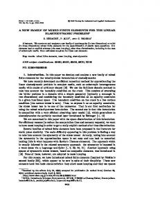
We discretize the domain using a coarse tensor-product mesh. The in-plane triangulation T x consists of 16 elements, in thickness direction we use one to four elements. This implies that the mesh size in thickness direction varies from hz = dz to hz = 0.25 · dz . We first do all computations for dz = 0.1, so the aspect ratio of the domain is 1/10. We use adaptive refinement in x-direction, but keep the mesh size fixed in z-direction. We use finite element spaces of orders one and two. In Figure 4, we plot the error against the number of degrees of freedom. The different curves correspond to different discretizations with respect to the z-direction using one, two and four elements in thickness direction. As expected, a linear or quadratic rate of convergence is achieved in the first refinement steps, indicated by the slope of the error curve almost parallel to the given reference slopes. For the different discretizations with respect to z-direction, the error curve saturates at different points. This saturation happens as soon as the total error is dominated by the error due to the mesh size hz .In Figure 5, we used a plate of thickness dz = 0.01, and one element in thickness direction. Again, we plot the error using adaptive refinement in x-direction, and find the almost optimal order of convergence. Moreover, we apply the p-version of the finite element method. We use the same coarse mesh as for the h-version, but perform one level of geometric refinement towards the sides of the plate. We keep this mesh fixed, and do calculations for increasing polynomial order, namely k = 1, . . . 4. We see the exponential convergence one generally expects for high-order methods, although exponential convergence with respect to the polynomial degree was not shown rigorously in the current work. The stability proofs in Section 3 may thus be not optimal. Our next example is a cylindrical shell of thickness dz = 0.01. We discretize the shell by prismatic, curved elements, where the order of the element mapping is equal to the order of the underlying finite element spaces. Note that curved elements are not covered by the theory in the previous sections. We used both our mixed finite elements, as well as a standard primal H 1 conforming discretization. For the standard primal method, we choose elements of polynomial order k = 5, while for the new mixed method elements of order k = 3 are used. The standard discretization leads to 49 722 coupling degrees of freedom, while for the proposed mixed methods, 42 451 coupling degrees of freedom arise. In Figure 6, we plot the absolute value of the stress |σ|. Clearly, the mixed method leads to better results even though the polynomial order is chosen lower than for the standard method.
ANISOTROPIC MIXED FINITE ELEMENTS FOR ELASTICITY
27
hz = 0.1 hz = 0.05 hz = 0.025 linear
0.01
0.005
0.002 2000
5000 10000
0.01
50000 100000 hz = 0.1 hz = 0.05 hz = 0.025 quadratic
0.005
0.001 2000
5000
10000
50000 100000
Figure 4. Estimated error vs. degrees of freedom for a square plate of thickness dz = 0.1, with one, two and four elements in transverse direction (hz = 0.1, 0.05 and 0.025), top order k = 1, bottom order k = 2. Acknowledgements Both authors acknowledge support from the Austrian Science Foundation FWF within project grant Start Y-192, “hp-FEM: Fast Solvers and Adaptivity” References [1] Alessandrini SM, Arnold DN, Falk RS, Madureira AL. Derivation and justification of plate models by variational methods. In Plates and Shells (Quebec 1996), vol. 21 of CRM Proceeding and Lecture Notes, Fortin M (ed). AMS, Providence RI, 1999; 1-20. [2] Arnold DN, Awanou G, Winther R. Finite elements for symmetric tensors in three dimensions. Math. Comp. 2008; 77(263):1229-1251. [3] Adams S, Cockburn B. A mixed finite element method for elasticity in three dimensions. J. Sci. Comput. 2005; 25(3):515-521.
2 ¨ A. PECHSTEIN1 AND J. SCHOBERL
28
k=1 k=2 geom. ref., p−version linear quadratic
0.02
0.01
0.005
2000
5000
10000
50000
100000
Figure 5. Estimated error vs. degrees of freedom for a square plate of thickness dz = hz = 0.01, order k = 1, 2 with adaptive refinement, and p-version FEM (orders k = 1, . . . 4) for prescribed mesh with one level of geometric refinement.
Figure 6. Cylindrical shell, absolute value of the stress |σ|,range 0 to 0.05 N/m2 , left: standard primal method of order 5, right: new mixed method, order 3 [4] Arnold DN, Falk RS, Winther R. Mixed finite element methods for linear elasticity with weakly imposed symmetry. Math. Comp 2007; 76(260):16991723. [5] Ainsworth M. A posteriori estimation for fully discrete hierarchical models of elliptic boundary value problems on thin domains. Numer. Math. 1998; 80: 325-362.
ANISOTROPIC MIXED FINITE ELEMENTS FOR ELASTICITY
29
[6] Arnold DN, Winther R. Mixed finite elements for elasticity. Numer. Math 2002; 92:401-419. [7] Buffa A, Ciarlet P Jr. On traces for functional spaces related to Maxwell’s equations Part I: An integration by parts formula in Lipschitz polyhedra. Math Methods Appl. Sci. 2001; 24(1):9-13. [8] Buffa A, Ciarlet P Jr. On traces for functional spaces related to Maxwell’s equations Part II: Hodge decompositions on the boundary of Lipschitz polyhedra and applications. Math Methods Appl. Sci. 2001; 24(1):31-48. [9] Brezzi F, Fortin M. Mixed and Hybrid Finite Element Methods. SpringerVerlag: New York, 1991. [10] Babuˇska I, Li L. Hierarchic modeling of plates. Computers and Structures 1991; 40:419-430. [11] Braess D. Finite Elemente: Theorie, schnelle L¨ oser und Anwendungen in der Elastizit¨ atstheorie. Springer Verlag: Berlin, 1992. [12] Brenner S. Korn’s inequalities for piecewise H 1 vector fields. Mathematics of Computation 2004; 73:1067-1087. [13] Brenner SC, Scott LR. The Mathematical Theory of Finite Element Methods. Springer-Verlag: New York, 2002. [14] Cl´ement P. Approximation by finite element functions using local regularization. R.A.I.R.O. Anal. Numer. 1975; 9:77-84. [15] D¨ uster A, Br¨oker H, Rank E. The p-version of the finite element method for three-dimensional curved thin walled structures. Int. J. Num. Meth. Eng. 2001; 52:673-703. [16] Demkowicz L, Kurtz J, Pardo D, Paszy´ nski M, Rachowicz W, Zdunek A. Computing with hp-adaptive finite elements. Vol. 2. Chapman & Hall/CRC Applied Mathematics and Nonlinear Science Series, 2008. [17] Duvaut G, Lions JL. Inequalities in Mathematics and Physics. Springer-Verlag: Berlin Heidelberg New York, 1976. [18] Dupont T, Scott R. Polynomial approximation of functions in Sobolev spaces. Math. Comp. 1980; 34(150):441-463. [19] Koiter WT. A consistent first approximation in the general theory of thin elastic shells. In Proc. Sympos. Thin Elastic Shells (Delft, 1959). North-Holland: Amsterdam, 1960; 12-33. [20] Dauge M, Faou E, Yosibash Z. Plates and shells: Asymptotic expansions and hierarchical models. In Encyclopedia of Computational Mechanics. Volume I. Stein E, de Borst R, Hughes TJR (eds). 2004; 199-236. [21] Mindlin RD. Influence of rotatory inertia and shear flexural motions of isotropic elastic plates. J. Appl. Mech. 1951; 18:31-38. [22] Monk P. Finite element methods for Maxwell’s equations. Claredon Press: Oxford, 2003. [23] Mardal KA, Winther R. An observation on Korn’s inequality for nonconforming finite element methods. Math.Comp. 2006; 75(253):1-6. [24] N´ed´elec JC. Mixed finite elements in R3 . Numer. Math. 1980; 35:315-341. [25] N´ed´elec JC. A new family of mixed finite elements in R3 . Numer. Math 1986; 50:57-81. [26] Nitsche JA. On Korn’s second inequality. RAIRO Anal. Num´er. 1981; 15(3):237-248.
2 ¨ A. PECHSTEIN1 AND J. SCHOBERL
30
[27] Reissner E. The effect of transverse shear deformation on the bending of elastic plate models. J. Appl. Mech. 1945; 12:69-76. [28] Reissner E. On a variational theorem in elasticity. J. Math. Physics 1950; 29:90-95. [29] Schwab C. A-posteriori modeling error estimation for hierarchic plate models. Numer. Math. 1996; 74:221-259. [30] Sch¨oberl J. Commuting quasi-interpolation operators for mixed finite elements. Report ISC-01-10-MATH, Texas A&M University; 2001. [31] Sinwel A. A New Family of Mixed Finite Elements for Elasticity. PhD thesis, Institut f¨ ur Numerische Mathematik, Johannes Kepler University Linz, Austria, 2009. [32] Stein E, Ohnimus S. Coupled model- and solution-adaptivity in the finiteelement method. Comput. Methods Appl. Mech. Engrg., Symposium on Advances in Computational Mechanics, Vol. 2 (Austin, TX, 1997) 1997; 150(14):327-350. [33] Sch¨oberl J, Sinwel A. Tangential-Displacement and Normal-Normal-Stress Continuous Mixed Finite Elements for Elasticity. submitted. [34] Scott LR, Zhang S. Finite element interpolation of nonsmooth functions satisfying boundary conditions. Math. Comp 1990; 54(190):483-493. [35] Sch¨oberl J, Zaglmayr S. High order N´ed´elec elements with local complete sequence properties. COMPEL 2005; 24(2):374-384. [36] Timoshenko SP, Woinowsky-Krieger S. Theory of plates and shells (2nd ed). Engineering Societies Monographs, New York: McGraw-Hill, 1959. [37] Vogelius M, Babuˇska I. On a dimensional reduction method. I. The optimal selection of basis functions. Math. Comp. 1981; 37(155):31-46. [38] Zaglmayr S. High Order Finite Element Methods for Electromagnetic Field Computation. PhD thesis, Institut f¨ ur Numerische Mathematik, Johannes Kepler University Linz, Austria, 2006. 1
Institute of Technical Mechanics, Johannes Kepler University Linz, Altenbergerstr. 69, 4040 Linz, Austria,, 2 Institute for Analysis and Scientific Computing, Vienna University of Technology, Wiedner Hauptstrasse 8-10, 1040 Wien, Austria