less suited to real time application, often requiring all training data to be ... system, called ADMIT (Anomaly-based Data Mining for InTrusions), relaxes these.
ANOMALY-BASED DATA MINING OF INTRUSIONS By Karlton David Sequeira A Thesis Submitted to the Graduate Faculty of Rensselaer Polytechnic Institute in Partial Fulfillment of the Requirements for the Degree of MASTER OF SCIENCE
Approved:
Prof. Mohammed J. Zaki Thesis Adviser
Rensselaer Polytechnic Institute Troy, New York April 2002 (For Graduation May 2002)
CONTENTS LIST OF TABLES . . . . . . . . . . . . . . . . . . . . . . . . . . . . . . . . .
iv
LIST OF FIGURES . . . . . . . . . . . . . . . . . . . . . . . . . . . . . . . .
v
ACKNOWLEDGMENT . . . . . . . . . . . . . . . . . . . . . . . . . . . . . .
vi
ABSTRACT . . . . . . . . . . . . . . . . . . . . . . . . . . . . . . . . . . . . vii 1. INTRODUCTION . . . . . . . . . . . . . . . . . . . . . . . . . . . . . . . 1.1
1
Background . . . . . . . . . . . . . . . . . . . . . . . . . . . . . . . .
1
1.1.1
Evaluation of IDS . . . . . . . . . . . . . . . . . . . . . . . . .
2
1.1.2
Categorization of IDS . . . . . . . . . . . . . . . . . . . . . . .
3
Research Goals . . . . . . . . . . . . . . . . . . . . . . . . . . . . . .
5
1.2.1
Basic requirements of IDS . . . . . . . . . . . . . . . . . . . .
5
1.2.2
Specific goals . . . . . . . . . . . . . . . . . . . . . . . . . . .
6
2. ADMIT: DESIGN PRINCIPLES AND RELATED WORK . . . . . . . . .
8
1.2
2.1
Theoretical functionality of IDS . . . . . . . . . . . . . . . . . . . . .
8
2.2
Alternatives for IDS Implementation . . . . . . . . . . . . . . . . . .
8
2.2.1
Detection Approach . . . . . . . . . . . . . . . . . . . . . . . .
9
2.2.2
Data Collection Granularity . . . . . . . . . . . . . . . . . . .
9
2.2.3
Data Model . . . . . . . . . . . . . . . . . . . . . . . . . . . . 10
2.2.4
Data Collection and Processing Location . . . . . . . . . . . . 10
2.3
Related Work . . . . . . . . . . . . . . . . . . . . . . . . . . . . . . . 12 2.3.1
User-profile based intrusion detection . . . . . . . . . . . . . . 12
2.3.2
Anomaly based intrusion detection 2.3.2.1 Quantitative analysis . . . 2.3.2.2 Statistical analysis . . . . 2.3.2.3 Non-linear analysis . . . .
2.3.3
Clustering-based anomaly detection . . . . . . . . . . . . . . . 15
. . . .
. . . .
. . . .
. . . .
. . . .
. . . .
. . . .
. . . .
. . . .
. . . .
. . . .
. . . .
. . . .
. . . .
. . . .
12 13 13 14
3. ADMIT ARCHITECTURE . . . . . . . . . . . . . . . . . . . . . . . . . . 18 3.1
Distributed data collection . . . . . . . . . . . . . . . . . . . . . . . . 18
3.2
Distributed data processing . . . . . . . . . . . . . . . . . . . . . . . 19
3.3
Software Architecture . . . . . . . . . . . . . . . . . . . . . . . . . . . 20 ii
4. ADMIT ALGORITHMS . . . . . . . . . . . . . . . . . . . . . . . . . . . . 24 4.1
Sequence Similarity Metric . . . . . . . . . . . . . . . . . . . . . . . . 24
4.2
Dynamic Training . . . . . . . . . . . . . . . . . . . . . . . . . . . . . 26
4.3
4.2.1
Data Pre-processing . . . . . . . . . . . . . . . . . . . . . . . 26
4.2.2
Clustering Algorithms . . . . . . . . . . . . . . . . . . . . . . 27
4.2.3
Cluster Refinement . . . . . . . . . . . . . . . . . . . . . . . . 31
4.2.4
Parameter Setting
. . . . . . . . . . . . . . . . . . . . . . . . 32
Online Testing . . . . . . . . . . . . . . . . . . . . . . . . . . . . . . . 33 4.3.1
Data Pre-processing . . . . . . . . . . . . . . . . . . . . . . . 33
4.3.2
Profile Search . . . . . . . . . . . . . . . . . . . . . . . . . . . 33
4.3.3
Sequence Rating Metric . . . . . . . . . . . . . . . . . . . . . 34
4.3.4
Sequence Prediction . . . . . . . . . . . . . . . . . . . . . . . 36 4.3.4.1 Online Anomalous Sequence Clustering . . . . . . . . 37
5. EXPERIMENTAL STUDY . . . . . . . . . . . . . . . . . . . . . . . . . . 39 5.1
Experimental Data . . . . . . . . . . . . . . . . . . . . . . . . . . . . 40
5.2
Base-line experiments . . . . . . . . . . . . . . . . . . . . . . . . . . . 40
5.3
5.2.1
Experimental Setup . . . . . . . . . . . . . . . . . . . . . . . . 40
5.2.2
Effect of Sequence Length . . . . . . . . . . . . . . . . . . . . 41
5.2.3
Effect of Clustering algorithm . . . . . . . . . . . . . . . . . . 43
5.2.4
Effect of Training Data Size . . . . . . . . . . . . . . . . . . . 44
5.2.5
Effect of Sequence Rating Metric . . . . . . . . . . . . . . . . 44
5.2.6
Sensitivity Variation . . . . . . . . . . . . . . . . . . . . . . . 45
5.2.7
Effect of Intra-cluster Threshold . . . . . . . . . . . . . . . . . 46
5.2.8
Effect of Test Data Size . . . . . . . . . . . . . . . . . . . . . 47
5.2.9
Effect of Similarity Metric . . . . . . . . . . . . . . . . . . . . 48
Real-time experiments . . . . . . . . . . . . . . . . . . . . . . . . . . 49 5.3.1
Detecting Concept Drift . . . . . . . . . . . . . . . . . . . . . 50
5.3.2
Segregating OTHER concepts from SELF profile . . . . . . . . 53
6. CONCLUSIONS AND FUTURE WORK . . . . . . . . . . . . . . . . . . . 56 6.1
Conclusions . . . . . . . . . . . . . . . . . . . . . . . . . . . . . . . . 56
6.2
Future Work . . . . . . . . . . . . . . . . . . . . . . . . . . . . . . . . 56
BIBLIOGRAPHY . . . . . . . . . . . . . . . . . . . . . . . . . . . . . . . . . 58
iii
LIST OF TABLES 5.1
DynamicClustering v/s KmeansClustering : Accuracy and TTA . . . . 43
5.2
DynamicClustering v/s KmeansClustering : Time, Alarm B and cluster growth Rate . . . . . . . . . . . . . . . . . . . . . . . . . . . . . . . . . 44
5.3
Testing on mixed data without real-time learning . . . . . . . . . . . . . 51
5.4
Testing on mixed data with real-time learning on a maximum of 250 sequences . . . . . . . . . . . . . . . . . . . . . . . . . . . . . . . . . . . 52
5.5
Testing on mixed data with real-time learning and all sequences . . . . 53
iv
LIST OF FIGURES 3.1
ADMIT’s Architecture: Training/Testing . . . . . . . . . . . . . . . . . 21
5.1
Effect of Sequence Length . . . . . . . . . . . . . . . . . . . . . . . . . . 42
5.2
Sequence Length: Time, Cluster Support . . . . . . . . . . . . . . . . . 43
5.3
Effect of Training Data Size . . . . . . . . . . . . . . . . . . . . . . . . 45
5.4
Effect of Rating Metric . . . . . . . . . . . . . . . . . . . . . . . . . . . 46
5.5
Effect of Sensitivity . . . . . . . . . . . . . . . . . . . . . . . . . . . . . 47
5.6
Effect of Intra-cluster Threshold . . . . . . . . . . . . . . . . . . . . . . 48
5.7
Effect of Test Data Size . . . . . . . . . . . . . . . . . . . . . . . . . . . 49
5.8
Effect of Similarity Metric . . . . . . . . . . . . . . . . . . . . . . . . . 50
5.9
Real-time Learning . . . . . . . . . . . . . . . . . . . . . . . . . . . . . 55
v
ACKNOWLEDGMENT A Master’s thesis is generally the first really important piece of research for a graduate student. And to stay motivated through it is far easier with the encouragement and support of others. I would hence like to thank my advisor Prof. Mohammed Zaki for the encouragement and ideas he provided during this thesis. Also, I must credit him with nurturing my interest in data mining enough, to choose this field. I would also like to thank the people in the Secure Systems Group at Pitney Bowes, for supporting me through this work, especially Dr. Matthew Campagna, Brad Hammell, and Darryl Rathbun for their insightful information on how computer security is compromised. I would also like to thank Mr. John Winkleman, for the opportunity he provided me at Pitney Bowes to embark on this research. I would also like to thank the other co-ops at Pitney Bowes viz. Michael Jarrett and Hamid Ghadaki for being a great sounding wall for me to bounce off ideas. I also am grateful to Dr. Terran Lane, from the MIT AI Laboratory, for providing me with the data, from the work he had earlier done in this field. Finally, I would like to thank my family, especially my parents, who made what I am today, my brother and my sisters for their advice.
vi
ABSTRACT Security of computer systems is essential to their acceptance and utility. Computer security officers use intrusion detection systems to assist them in maintaining computer system security. This thesis deals with the problem of differentiating between masqueraders and the true user of a computer terminal. Prior efficient solutions are less suited to real time application, often requiring all training data to be labeled, and do not inherently provide an intuitive idea of what the data model means. The system, called ADMIT (Anomaly-based Data Mining for InTrusions), relaxes these constraints, by creating user profiles using semi-incremental techniques. It is a realtime intrusion detection system with host-based data collection and processing. Our method also suggests ideas for dealing with concept drift.
vii
CHAPTER 1 INTRODUCTION Security of computer systems is vital to their utility and acceptance. However, the threat was not taken seriously until the Morris worm in November 1988, which caused the Internet to be unavailable for five days [13]. Despite much work since then, the problem is far from solved. According to the 2000 Computer Security Institute/FBI computer crime study, 85% of the 538 companies surveyed, reported an intrusion or exploit of their corporate data, with 64% suffering a loss [30]. Thus, intrusion detection systems are becoming increasingly important.
1.1
Background Intrusion detection is defined [34] as “the problem of identifying individuals
who are using a computer system without authorization (i.e. “crackers”) and those who have legitimate access to the system but are abusing their privileges (i.e. the “insider threat”)”. Conventionally, computer security experts attempted to provide security through configuration, preventive design and by developing operation techniques to make intrusion difficult [18]. In 1980, it was suggested [3], that audit data, initially collected for accounting purposes, could be analyzed to detect security violations. In the 80s, widespread networks hardly existed and the overhead of a real-time system seemed too high a cost. Hence, batch-mode systems were fairly acceptable. However, despite the availability of processing power having increased by several orders of magnitude since then, the problem of overhead is far from over, as the amount of information passed over networks and the very size of these networks has also been increasing exponentially. Also, computer systems can nowadays be compromised in a matter of seconds by non-experts, using new and ever-changing methods. Thus, the need for new methods to protect computer systems. The quantity of traffic makes it obligatory for network administrators and network security experts to use specific tools, called intrusion detection systems 1
2 (IDS), to prune down the monitoring activity they require to do. Security of computer systems may be compromised to different extents depending on the location of compromise [16] viz. 1. Physical Intrusion - in which the intruder has physical access to an unmonitored console with sufficient privileges. This is the hardest to detect and respond to. 2. System Intrusion - in which users with certain privileges abuse them to gain further privileges. 3. Remote Intrusion - where intruders remotely penetrate the system with initially no privileges at all. Generally intruders get into systems by making use of software bugs (buffer overflows, unhandled input, poorly multithreaded programs), faulty system configuration (lazy administrators, using default configurations, exploiting “trust relationships” to increase privileges, accidental hole creation), password cracking (using dictionary/ brute force attacks), sniffing unsecured traffic (e.g. sniffing telnet traffic can uncover passwords easily as they are not encrypted) and design flaws (TCP/IP design flaws, UNIX design flaws). 1.1.1
Evaluation of IDS The IDS are evaluated on the basis of its accuracy, efficiency and usability [32]
The characteristics used to evaluate the accuracy of the IDS are: 1. Detection Rate: It is the percentage of attacks that a system detects. 2. False Positive Rate: It is the percentage of normal data that the system incorrectly determines to be intrusive. The plot of the detection rate against the false positive rate is used to compare accuracy of different IDS. The plot is called the Receiver Operating Characteristic (ROC) curve. The accuracy gives a measure of the ability of the IDS to handle noisy, discrete data and to adapt. Other bases for evaluation include:
3 1. Time-to-alarm(TTA) [28]: It is the mean time to alarm generation. It is a measure of the sensitivity of the system. It determines the efficacy of the system to detect intrusions in real time. 2. Data reduction: It is the ratio of the data, the security analyst has to go through, to the size of the audit data. This system aims to reduce the work of the security analyst by reducing the data he has to sift through. It is a measure of the system’s usability. All these measures together reflect the suitability of the data model and algorithms adopted, to the domain of this problem. 1.1.2
Categorization of IDS IDS may be dichotomized on the basis of a number of characteristics [4] viz.
1. Detection Approach: IDS may be either (a) Anomaly Detection-based: e.g. AAFID [43], EMERALD [36], etc. Anomaly detection is performed, by searching for aberrations from previously observed usage patterns. (b) Misuse Detection-based: e.g. IDIOT [27], DIDS [42] etc. Misuse detection is performed, by searching for patterns known to be indicative of attacks/intrusions (known as signatures). (c) Hybrid of both anomaly and misuse detection: e.g. IDES [10], Haystack [40], etc. 2. Learning Approach: IDS may be either: (a) Self-learning: e.g. IDES [10], EMERALD [36], etc. Self-learning systems are those, that learn via observation, as to what constitutes normal/abnormal behavior. They can adapt as the behavior changes. (b) Programmed: e.g. DIDS [42], IDIOT [27], etc. Programmed systems require to have their parameters set by a programmer i.e. they increase human intervention and are not as adaptable.
4 However self-learning systems are generally easier to fool and can be trained to recognize the “intrusion” as “normal”. 3. Reaction on intrusion detection. IDS may be: (a) Active: EMERALD [36], etc. Active IDS can react by shutting down services/parts of the network, shutting off the TCP connection, logging more audit data, using retaliatory attacks (probably illegal), redirecting to ”honeypots”, notifying the ISP of source of attack, etc. (b) Passive: DIDS [42], IDIOT [27], etc. Passive IDS only generate alarms. 4. Data collection location. IDS may be: (a) Centralized Data Collection: IDIOT [27], Haystack [40], etc. In centralized data collection, data is typically read from a LAN and easier to manage. (b) Distributed Data Collection: DIDS [42], AAFID [43], etc. Distributed data collection typically involves sniffing of data at the host level and their summaries being fed to the higher level. 5. Detection Time. IDS may be: (a) Real-time/Near real-time: DIDS [42], IDIOT [27], etc. Real-time /near real-time intrusion detection is essential to rapidly respond to attacks. These are generally running continuously. (b) Periodical/Non-real time: Haystack [40], GrIDS [16], etc. Periodical IDS or systems that batch-process data are used to learn of new attacks. These generally work on a batch of traces at a time. 6. Data processing location. IDS may be: (a) Centralized: IDIOT [27], Haystack [40], etc.
5 (b) Distributed: HOBIDS [1], AAFID [43] etc.
1.2
Research Goals It is our belief that current IDS techniques are not sophisticated enough to
completely automate the intrusion detection problem, and that expert human supervision is ultimately necessary. Hence, we try to minimize the work of the intrusion analyst by providing likely alarms, rather than completely automating the process. Also, we must clarify that we believe that computer security, being the hard problem it is, can be achieved only through a layered approach, with each layer tackling different types of problems. This idea is referred to in computer security circles as “defense in depth”. Ours would be one of these layers, to prevent masquerades. 1.2.1
Basic requirements of IDS To build a powerful IDS, it is necessary to enumerate the desirable character-
istics [43] : 1. It must run continually. It must run in the background of the system being monitored. The security analyst must always be able to monitor its status. 2. Fault tolerance - ability to recover from system crashes and reinitializations. Crashes must not require retraining or relearning of rules/behavior. 3. Imperviousness to subversion - the IDS itself must not be vulnerable. The system must ideally be able to monitor itself to avoid subversion. 4. Scalability - the IDS must be able to handle the load as the network grows. 5. Adaptability - as the user behavior and system changes over time. e.g. a printer, which earlier served department A, maybe used to serve departments A and B, due to a breakdown of department B’s printer. A user may be assigned to a new work shift causing the timestamps of his usage patterns to change sharply.
6 6. Minimal overhead - on systems/hosts running relevant programs. The more the overhead, the less the possibility of acceptance. Host-based systems tend to be the worst affected by this. The overhead may be either by consuming too much memory (primary or secondary) or CPU cycles. 7. Configurability - the IDS must be able to be configured according to the desired security policies, preferably dynamically. 8. Graceful degradation of service - if some component crashes, the entire system must not crash. Other challenges [28] to contend with are: 1. Noisy data: A user may mistype a password accidentally or postpone an activity due to some interruption. This data could be misunderstood to be an intrusion, as it is an anomaly. 2. Audit data requirements: Determining the type of data required to closely model a system/user/resource usage is extremely hard. 3. Audit data types: Audit data may have categorical (e.g. command name), discrete (number of password logins), continuous (timestamps) values. Comparing categorical values of different records is difficult. 4. Audit data dimensionality: Audit data records have a large number of attributes. This increases the complexity of the problem considerably. Hidden Markov Models (HMMs) have been shown to effectively model system call data, but they take very long to do so as they are dependent on the dimensionality of the data [46]. 1.2.2
Specific goals The specific problem, we wish to tackle through our IDS is, the identification
of masqueraders, i.e. individuals who pass themselves off to be a particular person, but do not behave in a manner, that person is expected to. Besides the goals already mentioned, there are certain subgoals, that we have paid particular attention to.
7 1. Faster training: Neural networks and hidden Markov Models, generally require large amounts of training data for a good model to be realized. Also, models thus gained cannot be used directly to improve training for other users. We pursue a model that inherently satisfies these requirements. 2. Concept drift: Over periods of time, the user’s profile may change, due to a different agenda e.g. the user’s skill may improve and typographical errors will decrease, the user may be required to work with a new set of tools due to a project change etc. Hence, what is part of his/her profile might not be required to be part of the profile tomorrow. This is called “concept drift”.
CHAPTER 2 ADMIT: DESIGN PRINCIPLES AND RELATED WORK In this chapter, we discuss the different design alternatives for implementing an IDS, the drawbacks and advantages noticed within them and the ideas prescribed by past and contemporary work. We outline the alternatives we have chosen and the reasons and tradeoffs involved in doing so.
2.1
Theoretical functionality of IDS Detecting masquerades is a prediction problem i.e. given the audit data of a
user, we are required to predict whether more audit data is generated by the same person or not. The audit data known to have originated from the user, is called the “training” data and that, whose origin is to be predicted, is called “test data”. To predict the origin of the test data, it is necessary to first create a good model, p, of the user behavior from the given training data. After doing so, we must derive a mapping from the input space i.e. test data to the label i.e. “masquerader” or “user”, by using the model p. The training and test data have the same alphabet i.e. the alphabet of the audit data A. Thus, more formally, we seek to find functions φ and ψ, such that ψ : A+ → p φ : (A+ , p) → {“masquerader”, “user”} Thus, the IDS must implement two functions ψ and φ.
2.2
Alternatives for IDS Implementation Now that the functionality of the IDS has been specified, we mention the al-
ternatives available to go about implementing it. In 1.1.2, we described the basis for dichotomization of different IDS. These categories also correspond to the alternatives while implementing an IDS.
8
9 2.2.1
Detection Approach The IDS alternatives on the basis of detection approach are :
1. Anomaly-detection based. 2. Misuse detection based. 3. Hybrid of anomaly and misuse detection. Anomaly detection-based systems are designed to detect previously unobserved intrusions and hence are adaptable as compared to misuse detection-based systems . However, they are susceptible to changing user patterns and hence tend to have a higher false positive rate. Also, if they are statistically based, as a majority of them are, they have a problem with initialization i.e. before there is training data, the system is easy to manipulate and if they are exploited then, they can be trained by intruders to recognize the “intrusion” as “normal”. Misuse-detection based IDS monitor for a number of intrusion-prone patterns, whose number are only likely to increase as time passes and number of applications and exploits increase, hence it does not scale so well as anomaly-based methods. Anomalybased IDS learn what is “normal” while misuse-based IDS are told what is “intrusive”. Misuse-based IDS do not have an initialization problem. The hybrid methods are the best as they utilize the good points of both detection methods. They detect anomalies and use them to complement signatures to detect both known and unknown intrusions. 2.2.2
Data Collection Granularity These alternatives pertain to the granularity level at which audit data must
be collected. Too granular data may impose too high an overhead, on the machine processing it and too coarse data may not allow good enough models to be created . IDS alternatives on the basis of audit data collection granularity are: 1. Network level data e.g. [44, 31] 2. System-call level data e.g. [22, 31]
10 3. User command-level data e.g. [28, 11, 39] Most of the early and a lot of contemporary work in IDS focusses on network - level data to detect remote attacks. However, this kind of data does not completely solve out problem, because a poorly chosen password may be guessed, an authorized user may turn hostile, or a terminal may be left unattended, allowing an intruder to gain access without abusing the network. System-call level data is far too fine grained, which increases overhead. Also, it is likely to have scalability constraints. User-command level data is less granular than system call-level data and hence imposes a lesser overhead. However, techniques as descibed in 3.3 are necessary to prevent overfitting the model and to enhance scalability. 2.2.3
Data Model This involves the implementation of the earlier mentioned ψ function. IDS
alternatives on the basis of data model are: 1. User profile based e.g. [28, 11, 39] 2. Non-user profile based e.g. [31, 22] User profile based IDS create a profile for the user, based on data known to be generated by that user. There are a number of data models used to generate this profile e.g. Neural networks [38], Hidden Markov Models [28] , Statistic-based models [11, 39], instance-based learners [28] etc. These are discussed in more detail in 2.3.2.3 Non-user profile based methods are used for modeling data to prevent intrusions other than those related to masquerades e.g. denial-of- service attacks etc, in which data per connection is too little to create a profile. Here, resource usage data is mined for patterns and rules are derived [31]. Thus, resource usage profiles are mined rather than user profiles. 2.2.4
Data Collection and Processing Location IDS alternatives on the basis of data collection and processing location are:
11 1. Centralized data collection and processing. 2. Distributed data collection and processing. In a centralized approach, imperviousness to subversion is easier to implement as there are less components to secure, but the penalty of failure is more severe. The cost of overhead is centralized, so we must have dedicated systems for this approach. This does not allow scaling, as the size of the network is likely to outgrow the capacity of the dedicated systems. If there is centralized data collection you must have inputs from the individual hosts as well. Also centralized data collection may result in a bottleneck for the network. Distributed data collection typically increases traffic as a result of a lot of communication between the different components. Centralized processing systems are easier to configure. It makes dynamic configuration and graceful degradation very difficult however. It tends to decrease the overhead on hosts, but requires dedicated hosts for it. Distributed processing can be of two types 1. Cluster-based processing - in which a cluster of hosts have their IDS-related processing done by one dedicated processor. In this, the scalability problem is solved by simply splitting the cluster into two if it becomes too large. 2. Host-based processing - in which each host does its own IDS-related processing and hence there is no scalability problem. However, this can cause a lot of processes to start up on the host [43], resulting in too much overhead, slowing down the host machine to a crawl. A real-time system, would require the iDS to stay in memory thereby taking up cache and other resources. Thus, distributed processing too, comes at a price. Distributed data processing increases traffic as they result in a lot of communication between the different components for integration of observations. Here, the coordination is a problem too. If the system is distributed, different parts are easier to separately and independently configure at different periods of time, unless there is a high level of coupling between the parts. Also, if a part of the system goes down, the others continue to operate.
12 After taking into account all the alternatives, we have designed ADMIT as a user-profile dependent, temporal sequence clustering based, real time intrusion detection system with host-based data collection and processing.
2.3
Related Work In this section we describe the work related to our design and the lessons learnt
from them. 2.3.1
User-profile based intrusion detection Smaha was among the first to use intrusion detection in Haystack [17], based
on a combination of anomaly and misuse detection, in a method similar to ours, where they generated per-user models based on observed user behavior and specified generic acceptable behavior for pre-specified groups of users. However, the system operated in batch-mode, by analyzing a session at a time using statistical methods. In her seminal paper on IDS, Denning [10] too, suggested a model which was a mixture of anomaly and misuse detection, based on statistics, gathered from user behavior to create user and group profiles. These statistics formed the basis of an expert-based rule systems which flagged deviations as possible intrusions. It was the first work that suggested the mining of the temporal nature of audit data. It also suggested a number of methods to model the user behavior including Markov process, multivariate, time series and mean and standard deviation modelling. 2.3.2
Anomaly based intrusion detection Within the domain of anomaly detection, there exist the following approaches:
1. Quantitative analysis 2. Statistical analysis 3. Non-linear analysis
13 2.3.2.1
Quantitative analysis
Quantitative analysis methods include threshold detection in which system and user activities are monitored by software sensors [26, 10]. These thresholds may be fixed or they may be dynamically set using statistical methods [11, 39, 41, 23, 28]. Crossing these thresholds, results in the triggering of an alarm. ADMIT, too uses thresholds, which if crossed, trigger alarms. Another quantitative analysis technique is that of target-based integrity checks [6] viz. system objects that should not change, are monitored. Tripwire, a commercial software, uses this technique by generating MD5 hashes for files and storing them in a database. It frequently regenerates the hash and if it does not match the stored hash, alarms are triggered. Another method is that by Schonlau and Karr [39], who observed that test data appended to the training data yields a smaller compressed file, if the test data is that of the true user. However, this method does not help the security officer determine the activities of the masquerader and hence is more of a black-box solution. 2.3.2.2
Statistical analysis
Statistic-based profiling mechanisms were initially very popular [10, 40]. Recently too, a lot of work has been done in them. DuMouchel [11], used process control charts to create fixed length command sequence-based user profiles. He created a command probability transition matrix for each user, relating the conditional probability that a particular command k was immediately preceded by a command j i.e. Pu (next command = k — previous command = j) for each user u. After training, on pilot data, which is assumed to be intrusion free, the initial center line and offset for determining out of control points for the chart is determined. By monitoring a user specified-length sequence of commands, if its deviation from the profiled behavior exceeded the upper control limit, an alarm was sounded. Eskin [14] used a “mixture model” statistical technique as described in [5] for modeling system call traces. A fixed order Markov chain is used to detect the probability distributions of intrusion (anomalous distribution) and normal (major-
14 ity distribution) sequences in a stream of system calls, corresponding to privileged programs with known exploits. Each sequence is generated from either one of these distributions. The probability that a sequence is an anomaly is analyst-specified and assumed to be small. Once the probability distributions are estimated, the change in the generative distribution of data, due to each sequence being believed to be generated by the anomalous distribution, rather than the normal distribution, is compared with a analyst-specified threshold. If the threshold is exceeded, the sequence is labeled as “anomaly” and it is permanently moved to the anomaly set. In eBayesTCP [44], Valdes et al monitor contiguous TCP sessions and log a number of interesting events (e.g. number of unique ports, error intensity , number of unique IP addresses). Using Bayesian inference [35] over configurable periods of time, it obtains a set of hypotheses for the session in consideration. This method enables adaptation by allowing creation of new hypotheses, if none existing justify current observations. Using decayed weights for older observations, it allows newer observations to bear more influence and hence increase adaptability. Also, once a hypothesis is labeled as “attack”, no amount of reverse training can fool the system, into believing it to be “normal”. The idea of using decayed weights is used in one of ADMIT’s sequence rating metrics (4.3.3) and can be used for scaling the profiles over time to maintain relevance. Schonlau and Theus [41], use a method based on the observation that commands not seen at the time of training, are unlikely to be seen at the time of testing. If a command is not used by a number of users, then it is all the more unpopular. They define a test statistic that supports the bias towards using commands seen in training data in the test data. 2.3.2.3
Non-linear analysis
Non-parametric analysis techniques include machine learning ideas. Lee et al [31] used a machine learning classifier, RIPPER, to produce a decision tree whose rules are used to classify sequences as “normal” and “abnormal”. Forrest et al used immunocomputing methods for modeling normal sequences. Ryan et al [38] use a neural network to create user profiles to detect masquerades. However, neural
15 networks tend not to convey to the operator, the cause of the alarm when it does occur. Hence, the need for specific neural networks for specific attacks [6]. Lane and Brodley [29], use an instance based learning-based technique, wherein, they use a similarity measure to reduce to a single dimension, the temporal sequences of unordered, discrete attribute traces of user activity. In doing so, they can compare the sequences to learn user behavior. To minimize false alarm rate, they introduced a concept of acceptable false alarm rate threshold (r). They statistically set upper and lower (to prevent replay attacks) bounds on the amount of deviation that constitutes a normal trace. All traces falling outside these thresholds were declared as anomalies. To counter the problem of concept drift, they evaluated a number of models that adapted linearly to drift trends. They used these models to determine the selection of parameters for thresholds. Lane [28], like Warrender et al [46] also tried HMMs to model user behavior, with significant success in decreasing the false positive rate. ADMIT closely resembles the approach taken by Lane et al. 2.3.3
Clustering-based anomaly detection This method actually belongs to the class of non-linear analysis. However
as our method involves clustering, we delve deeper into it, in this subsection. To counter the problem of model scaling as described by Lane [28], the alternative we have chosen is clustering. C lustering seeks to create subgroups, wherein every member of a subgroup by some distance metric, is similar to its subgroup’s other members and dissimilar with respect to members of the other subgroups. By using clustering on the user traces, we intend to summarize the user behavior. We plan to use incremental clustering to allow for changes in the user behavior so that the profile can adapt to concept drift [28] in real time. The clustering algorithms are dichotomized as [20] : 1. Partitioning-based: e.g. k-means [33], k-median, k-mode Partitioning-based methods construct a user-specified number of clusters (say k of them) from the samples (say n of them) provided, by randomly assigning one to each, until each cluster contains at least one sample. It then uses an iterative relocation technique to allocate samples to clusters to improve the
16 partitioning by reassigning the samples to different clusters in each iteration (say t ). These methods perform well under small datasets but do not scale as they have complexity O(nkt). Another disadvantage is that convergence is not assured. Also , knowledge of the number of clusters restricts their utility and accuracy. They also tend to produce spherical clusters only. Also, they tend to find local optima i.e. the accuracy is dependent on initial assignment of centers. 2. Hierarchical methods: e.g. linkage methods [24] Hierarchical methods either work from top-to-bottom (divisive) or vice versa (agglomerative), where they initially put all samples in one/different cluster (s) and then, using some criterion, in each iteration, to improve distinction, divide/merge clusters respectively. These methods scale better than partitioning methods but they too are generally at least quadratic in nature. Their main disadvantage is that they are irreversible i.e. once a division/merger takes place, they cannot be reassigned. Also they are guaranteed to converge. 3. Locality-based methods: e.g. DBSCAN [15] Locality-based methods use a heuristic to create clusters to group neighboring samples e.g. in DBSCAN [15], a sample may belong to a cluster so long as it has more than a threshold (say n) number of samples within a specified radius (r) of it. Thus, each sample in a cluster has n-nearest neighbors within a radius r of it. This has the advantage of producing non-spherical clusters, but like the other methods discussed above, this method too, does not produce good clusters if there is high-dimensional data. 4. Grid-based methods: e.g. STING [45] Grid-based methods partition the sample space into a finite number of cells and perform the clustering operations on each of the cells individually. Its key advantage is its reduced performance time and ease of conversion to a distributed problem. Its processing time is dependent on the number of cells in each dimension but independent of the number of samples.
17 Portnoy [37], used a variant of the single-linkage clustering technique to group network traces (TCPDUMP data) and classifies the clusters as “normal” or “intrusion” based on the assumptions that intrusions are anomalous by nature and normal data of all types is sufficiently represented in the traces . Hence all clusters labeled as anomalies are treated as intrusions. First, he normalized the data, as TCPDUMP data is multidimensional. Then, he used a Euclidean metric with equally weighted features for all continuous attributes and a constant for all discrete attributes that were dissimilar for the traces being compared. For clustering, he set a limit on the radius for the clusters. All instances exceeding the radius were allocated a new cluster, for which they became the definitive trace. This results in spherical clusters and setting of the radius limit is hard to justify. This method does not adapt to changing usage behavior. Lane [28] used clustering successfully to reduce the historical data required to create the user profile. For a similarity measure, he devised a couple of linear algorithms in which adjacent matches are rewarded either linearly or exponentially. Also, a noise suppression filter to remove randomness and noise in data is applied. The sample is assigned to the cluster it is the most similar to in the profile, and this similarity is defined as its similarity to the profile. Their clustering algorithm grows clusters incrementally and individually, by greedily selecting traces from the training data that increase the intra-cluster distance by a minimum until that distance reaches a local maximum. It then measures the mean radius and discards all points that exceed that radius and returns them to the trace pool again so they can be included in other clusters. The cluster is then re-represented by its mean radius and center and all associated traces are discarded. Then the clusters are selected sequentially to maximize the inter-cluster distance, until some threshold is reached.
CHAPTER 3 ADMIT ARCHITECTURE In this chapter, we elaborate on the architectural details, from a conceptual as well as a software perspective, of ADMIT. In 1.2.1, we described among the goals of an IDS, the importance of imperviousness from subversion, scalability, minimal overhead, configurability and graceful degradation of service. A substantial factor of the performance of the IDS in these dimensions, is related to its architecture. While, there have been no contributions from ADMIT in these fields, it is important to underline the principles and lessons learnt from other IDS architectures and the reasons behind choosing the alternative chosen. The main alternatives to be chosen from, as far as the IDS architecture goes were whether to use a distributed or centralized approach towards data collection and processing. The merits and demerits of these approaches have already been discussed in 2.2.4. In the following sections, we describe the other IDS architectures which have adopted the distributed approach.
3.1
Distributed data collection DIDS [42] used Haystack [40] and NSM [19] to build a comprehensive dis-
tributed IDS. It consists of : 1. DIDS director which coordinates the activities of the IDS based on aggregated reports from the host and LAN monitors, 2. Host monitors based on Haystack [40], which monitor each host, logs interesting events and communicates the same to the DIDS director and 3. LAN monitor for each LAN segment, which reports on interesting network activity to the DIDS director. However, this architecture involves centralized processing. 18
19 GrIDS [17] used a graph-based approach to represent network usage. Nodes represent hosts and connections between hosts are represented by edges. It uses activity graphs to determine the presence of network-wide coordinated attacks.
3.2
Distributed data processing AAFID [43], uses the idea of autonomous agents, which are functionally inde-
pendent entities having specific tasks assigned to each. They are allowed to perform any function they need. It was hoped that they may learn or evolve using genetic programming or machine-learning techniques as described in [9]. However, genetic programming is known to have problems like code bloat and they generally take longer to converge to a solution. Each agent starts up a separate process producing considerable overhead on the host. Also, scalability limits the number of agents concurrently running over a single host. Also, the intruder can potentially disable the agent by killing the corresponding process. To counter this, Zamboni et al [26] are in the process of developing a system involving sensors, each of which, is defined as “a piece of software (potentially aided by a hardware component) that monitors a specific variable, activity or condition of a program and that is an integral part of the program being monitored”. But this requires recompilation of the kernel (they used OpenBSD to prove the validity) and modifying all programs desired to be secure. The advantage is that they can never be disabled without disabling the program itself. The difficulty is in the deployment. Lee et al [31], too advocate the use of agents to distributedly monitor the system. They use a mixture of anomaly and misuse detection and train the data using ‘artificial’ anomalies (to allow more definite dichotomization between the classes), inserted into normal and intrusion traces. Each agent architecture involves three components : 1. A sensor that records system data and feeds it to the other components 2. An adaptive model generator that receives data from the sensor and generates a corresponding data model which it supplies as input to the 3. Detector, which using the model analyses data from the sensor and detects
20 and responds to intrusions. The adaptive data model generator consists of a data warehouse, data receiver, model generator and model distributor. Thus, different models may be learned on different hosts depending on the usage. This method also uses the work in [14] described earlier.
3.3
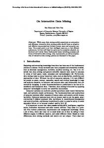
Software Architecture There are two main stages in our approach to mining intrusions. In the training
phase, the user profiles are created, and in the testing phase, the user command stream data is verified against the corresponding profile. The complete architecture of ADMIT is shown in Figure 3.1. User data enters the system by the monitoring of the UNIX shell command data [28], captured via the (t)csh history file mechanism. A recognizer for the (t)csh command language parses user history data and emits them as a sequence of tokens in an internal format. All commands between a user’s logging on and logging off are referred to as a user session and corresponding delimiters (*SOF* and *EOF*, respectively) are inserted to indicate the same. We process data within different sessions separately to avoid patterns created by coincidence across sessions from being incorporated into the user profiles. An example session could be : SOF*; ls -l; vi t1.txt; ps -eaf; vi t2.txt; ls -a /usr/bin/*; rm -i /home/*; vi t3.txt t4.txt; ps -ef; *EOF* (in the real data, instead of a ‘;’, we have a new line character). During training, the commands entered by a user are stored in that user’s audit data file according to the time of entry. During testing, the command data is directly used to detect anomalies via online sequential prediction. We consider each process/command in the history data together with its arguments as a single token (*SOF* and *EOF* are not considered to be tokens). However, to reduce the alphabet size, we omitted filenames in favor of a file count as in Lane [28]. For example, the user sequence given above is converted to the following sequence T = {ti : 0 ≤ i < 8}, where t0 = ls -l, t1 = vi , t2 = ps -eaf, t3 = vi , t4 = ls -a , t5 = rm -i , t6 = vi , and t7 = ps -ef. The notation gives the number of arguments (n) of a command. For instance,
21
PROFILE MANAGER Parameters Parameters Adds new
PROFILE CREATOR
Parameters
Parameters
Clusters FEATURE SELECTOR
CLUSTER CREATOR Sequences
Parameters
PROFILE UPDATER
User Profiles
Profile
SEQUENCE EXAMINER
updates
Parameters Unassigned Sequences Clusters CLUSTER FEATURE CREATOR SELECTOR
Process data Process data
User audit data TRAINING
Process data
User command stream TESTING
Figure 3.1: ADMIT’s Architecture: Training/Testing the command vi t1.txt is tokenized as vi , while rm t3.txt t4.txt as rm . However, options invoked during the execution of a command remain, as they help differentiate the skill level of users. Thus, ls -l data* becomes ls -l . ProfileManager is the top-level module in ADMIT; it is responsible for the security of a terminal. It has a number of deputies, whose operations it configures, coordinates and decides. ProfileCreator, during training, creates profiles for users authorized to use the terminal. ProfileUpdater updates profiles for those users during testing. SequenceExaminer examines each sequence of tokens of process data and determines if that is characteristic or not, of the user known to have produced it. Based on the decision, it takes action specified by the ProfileManager. The ProfileCreator and ProfileUpdater both use two sub-modules: 1. FeatureSelector: It parses the source command data for a user, cleans it up by replacing argument names by numbers (e.g., cat test.txt > sort becomes cat > sort) and converts it into tokens as described above. It then converts the token data from each session, into sequences of tokens, whose length is
22 specified by the ProfileManager. More formally, if T is the token alphabet, F eatureSelector : A+ → (T l )+
2. ClusterCreator: It converts the input array of sequences into clusters which form the profile of the user they originate from. Thus, the ProfileCreator, the FeatureSelector, the ClusterCreator and the ProfileManager collectively implement the ψ function to produce the profile which corresponds to the p in 2.1. At startup, the ProfileManager initializes the ProfileCreator, ProfileUpdater and SequenceExaminer with various parameters. At training time, the ProfileCreator instructs FeatureSelector, as to what data to parse, and how to clean and tokenize it. The FeatureSelector makes sequences out of the tokens, whose length is determined by the ProfileManager. Thus, a sequence s, of specified length l, is a list of tokens, occurring contiguously in the same session of audit data, i.e., s ∈ T l , where T is the token alphabet. The ProfileCreator then initializes the ClusterCreator and passes on the clustering algorithm and similarity measure, specified by the ProfileManager. If the parameters are to be set auomatically (see section 4.2.4), it then partitions the training sequences into two parts, where the ratio is user-specified. The first portion is generally the larger section and is called the training set. The remaining sequences are called the validation set. The ClusterCreator converts the sequences in the training set into clusters which are added to the user profile. The sequences in the validation set are then tested against the profile thus created and the lower accept threshold TACCEP T , as defined in 4.3.4, is estimated. The sequences in the validation set are then clustered, by the ClusterCreator and added to the profile. Thus, a cluster c, is a collection of sequences of user-initiated command data, such that all its sequences are very similar to others within itself, using some similarity measure Sim(), but different from those in other clusters . If the parameters are set by the user, the training sequences are clustered by the ClusterCreator and added to the profile directly.
23 If the clusters have sufficiently high intra-cluster similarity and low variance, the entire cluster may be represented by the center sequence. We define the center (denoted sc ) of a cluster as the sequence having the maximum aggregate similarity to the other sequences within the cluster. That is, if c = {s0 , s1 , . . . , sn−1 } is a cluster with n sequences, then sc = max{ si
n−1 X
Sim(si , sj )}
(3.1)
j=0
The clusters make up the profile for a given user. A profile p, is the set of clusters of sequences of user-initiated command data whose centers characterize the user behavior. Thus, for user u, pu = {ci |(Sim(sci , s) ≥ r, ∀s ∈ ci ) ∧ (Sim(sci , scj ) ≤ r ′ , i 6= j)}
(3.2)
where r and r ′ are the intra-cluster and inter-cluster similarity thresholds, respectively, sci is the center of cluster ci , and Sim(s1 , s2 ) is the similarity between two sequences. We expect pu to include several clusters to adequately capture the usage variations for user u. Having fine grained (but not overly so) clusters also allows us to reduce the false alarms while testing. Profiles thus created by the ProfileCreator, are added to the pool of user profiles P . During testing, the SequenceExaminer instructs FeatureSelector to parse, clean and tokenize command stream data of the user u currently logged in and convert them into sequences. These sequences are matched against the corresponding profile pu , obtained from the pool of user profiles P , by the ProfileUpdater. An alarm of type A may be sent to the security officer for each anomalous sequence. In contrast to the ProfileCreator’s ClusterCreator, only the anomalous sequences, deemed so by the SequenceExaminer, are clustered by the ProfileUpdater’s ClusterCreator. These can be added to user u’s profile pu .
CHAPTER 4 ADMIT ALGORITHMS In this chapter, we discuss the various algorithms used for implementing ADMIT.
4.1
Sequence Similarity Metric In 3.3, we described the similarity between sequences by the Sim function,
but deferred its specific implementation until now. We write the similarity between two categorical command sequences, s1 and s2 , as Sim(s1 , s2 ). More formally, Sim : T l × T l → ℜ , where T is the token alphabet and l is the length of the sequences. It is an atomic function of the clustering and prediction process ( described in detail in 4.2 and 4.3) and hence should be quick. Also, it is important to note that, we consider all commands to be of equal importance. The following similarity metrics have been proposed by Lane [28]: 1. MCP (Match Count Polynomial Bound) It counts the number of slots in the two sequences for which both have identical tokens and the count is the similarity score for the two sequences. For example, if s1 = { vi , ps -eaf, vi , ls -a }, and s2 = {vi , ls -a , rm -i , vi }, then MCP for s1 and s2 is 1 since they are identical only in the first slot. 2. MCE (Match Count Exponential Bound) It is a variant of MCP, in that it doubles its value for each matching position having an initial value of 1. Thus for the given MCP example, the similarity using MCE, is 2. 3. MCAP/MCAE (Match Count with Adjacency Reward and Polynomial/ Exponential Bound) 24
25 It is a variant of MCP/MCE [28], where adjacent matches are rewarded polynomially or exponentially respectively. Lane [28] reported that MCAP is typically better than the others, so we use that in our study. Another class of similarity metrics is designed on the basis of the dynamic programming paradigm. We considered, 1. the LCS metric (Longest Common Subsequence), which gives the length of the longest subsequence of tokens that the two sequences have in common. It too is polynomially bounded in the length l, i.e. O(l2 ) [8]. The disadvantage in LCS and MCP is that they produce a similarity metric having a whole value, which restricts the granularity of differentiation, i.e., Sim : T l × T l → [0, l]. 2. Hence, we devised the LCSA (Longest Common Subsequence with Additive adjacency reward) algorithm to counter this. This metric is analogous to MCAP from the match count-based class of similarity metrics. The LCSA algorithm is as follows, LCSA(s1 ,s2 ,i,j,α,β,AdjacencyReward): //s1 ,s2 are the sequences whose mutual similarity is to be determined //α is the reward for a single match //AdjacencyReward is the additional reward for an adjacent match //β is the increment in the AdjacencyReward 1. if(i=0 or j=0) return 0//termination of recursion 2. if(s1 [i] == s2 [j]), 3.
return LCSA(s1 ,s2 ,i-1,j-1,α,β,β + AdjacencyReward) + α + AdjacencyReward
4. else, 5.
return max(LCSA(s1 ,s2 ,i-1,j,α,β,0),LCSA(s1 ,s2 ,i,j-1,α,β,0) Thus, the LCSA algorithm is identical to the LCS one, except that LCS has β
= AdjacencyReward = 0, α = 1. LCSE (LCS with exponential adjacency reward) can be constructed from LCSA above, by changing line 3 to 3.
return LCSA(s1 ,s2 ,i-1,j-1,α,β,β * AdjacencyReward) + α + AdjacencyReward
26 While the dynamic programming similarity metrics mentioned are quadratic algorithms in comparison to the exact match-based linear algorithms in the length of the sequences, l, it is capable of representing similarity between phase-shifted sequences. For example, for the s1 and s2 described in the MCP example, LCS is 2, since they both share the subsequence vi , ls -a . The same result may be achieved using edit distance, dot-plots with the length of the longest diagonal corresponding to the similarity between the sequences and other sequence alignment algorithms used in bioinformatics[12].
4.2
Dynamic Training Initial user profiles in ADMIT are mined in the training phase from user com-
mands at their host machine. There are four main steps during training: 1. Data pre-processing, 2. Clustering user sequences, and 3. Cluster refinement. 4. Parameter Setting These steps are described in detail below. 4.2.1
Data Pre-processing ADMIT collects user audit data, by monitoring the command history files of
the users. It is necessary to clean the data prior to processing it and to convert it to a format, suitable for processing. We use the following history as a running example: SOF*; ls -l; vi t1.txt; ps -eaf; vi t2.txt; ls -a /usr/bin/*; rm -i /home/*; vi t3.txt t4.txt; ps -ef; *EOF* The FeatureSelector parses, cleans and tokenizes the audit data, within each session specified by the ProfileManager. As mentioned in 3.3, the cleaning involves replacing command arguments by their number, to fuzzify their specific instantiation. However, options e.g. -l for ls, are retained as they may indicate more about
27 the specific type of user i.e. a more experienced user of Unix is likely to use more options than a less experienced one. The above command stream results in the token list, T = {ti : 0 ≤ i < 8}, where t0 = ls -l, t1 = vi , t2 = ps -eaf, t3 = vi , t4 = ls -a , t5 = rm -i , t6 = vi , and t7 = ps -ef. The FeatureSelector next creates sequences of length l from the tokens based on the order of their creation time, as specified by the ProfileManager. For example, if l = 4, the set of user sequences is given as S = {si : 0 ≤ i ≤ |T | − l}, where: s0 = { ls -l, vi , ps -eaf, vi } s1 = { vi , ps -eaf, vi , ls -a } s2 = { ps -eaf, vi , ls -a , rm -i } s3 = {vi , ls -a , rm -i , vi } s4 = {ls -a , rm -i , vi , ps -ef }
4.2.2
Clustering Algorithms Once tokens have been converted into sequences, they are partitioned into
two parts, in a ratio specified by the user and conveyed by the ProfileCreator. As mentioned in 3.3, the first part is called the training set and the second, the validation set. We cluster each of the sets separately using a suitable clustering algorithm. In [21], Han et al enumerate three factors to be considered while choosing a clustering algorithm viz. application goal, characteristics of data and tradeoff between quality and speed. The given application involves a small sized dataset, as the smaller the training data, the more effective the process. Typically, the data sets size is about 1,500 sequences, which is not very large. However, the overhead on the host cannot be too high and hence the clustering algorithm chosen must have a resonable time and space complexity. Also, important to note is that the basic data set contains categorical data, hence comparisons should ideally be minimized. The dimensionality of the data often affects the performance of the clustering algorithm. In this application, the optimal dimensionality i.e. the length of the sequences, is
28 unknown. K-Means [33] is an often favored clustering algorithm because it allows reallocation of samples even after assignment and it converges quickly. It works as follows, K-meansClustering (t, K, pu , Su , Suc ): //t is the number of iterations //K is the number of clusters to be created //Su is a set of a user u’s sequences to be clustered //pu is the user u’s profile, i.e., set of clusters //Suc is the set of user u’s cluster centers 1. For each of the K clusters, 2.
Randomly select a sequence as center of the cluster,
i.e. si = random(Su ); ck = si ; Suc = Suc ∪ si 3. For t iterations 4. 5. 6. 7.
For each of the N = |Su | sequences, si ∈ Su For each of the K cluster centers, skc ∈ Scu find Sim(si , skc ) Assign si to the cluster it is the closest to.
i.e. ck = ck ∪ {si }, Sim(si , skc ) ≥ Sim(si , sjc ), 1 ≤ j ≤ K 8. 9.
For each of the K clusters, recalculate cluster center
10.For each of the K clusters, 11.
p u = p u ∪ ck The problem with basic k-means, besides those mentioned in 2.3.3, is that the
random allocation of cluster centers (line 2), reduces its accuracy, as it converges to a poor local optimum. Also, it is susceptible to noise and outliers , which can easily affect the centroid recalculation [20]. Also, k and t (number of iterations) are hard to set to achieve a good clustering. During each iteration, k-means first assigns each point to the closest cluster center (line 7) and then recalculates the cluster centers (lines 8 and 9). The first step takes time O(δkN), where δ is the cost of computing similarity between any two sequences. Recalculating the cluster centers
29 (lines 9) based on Equation 3.1 takes time O(δn2 ), and since there are k clusters, the time for the second step is O(δkn2 ) (with the simplifying assumption that all clusters have an equal number of points n). The cost of k-means per iteration is then given as δkN + δkn2 = O(δk(n2 + N)). Since there are t iterations, the total cost of k-means is O(tδk(n2 + N)). Note that for the match-based and dynamic programming-based similarity metrics, δ = O(l) and δ = O(l2 ), respectively. We do not want to use any preset value of k for the different users in our system. Thus instead of the basic k-means approach, we use a dynamic clustering approach to group a user’s sequences, where clusters are grown when needed, as shown in the pseudo-code below: DynamicClustering (r, Su , pu , Suc ): //r is intra-cluster similarity threshold //Su is a set of a user u’s sequences to be clustered //pu is the user u’s profile, i.e., set of clusters //Suc is the set of user u’s cluster centers 1. Sua = Su //set of user u’s “anomalous” sequences 2. while (Sua 6= ∅) //“anomalous” sequences exist 3.
select random sc ∈ Su − Suc as new cluster center
4.
cnew = {sc } //i.e., initialize new cluster
5.
Suc = Suc ∪ sc
6.
for all remaining sequences si ∈ Su − Suc
7. 8. 9. 10.
if (Sim(si , sc ) ≥ r) if ( Sim(si , s′c ) < Sim(si , sc )∀s′c ∈ Suc − sc ) cnew = cnew ∪ {si } recalculate cluster center, sc for cnew
11.
pu = pu ∪ cnew
12.
Sua = Sua − cnew Consider how DynamicClustering works on our example sequences. Initially
Su = Sua = {s0 , s1 , s2 , s3 , s4 }, pu = Suc = ∅, with r = 3. Within the while loop we
30 pick a random sequence as the new center, say s0 . For all remaining sequences in Su − Suc , where Suc = {s0 } we compute similarity to the new center s0 . Using LCS as the similarity metric we get Sim(s1 , s0 ) = 3 since vi , ps -eaf, vi is their LCS. For the other sequences we get: Sim(s2 , s0 ) = 2, Sim(s3 , s0 ) = 1, and Sim(s4 , s0 ) = 0. Since s1 passes the threshold, we add it to the new cluster to get cnew = {s0 , s1 }. Now the new Sua = {s2 , s3 , s4 } and we repeat the while loop. After a few steps we may find that the profile is given as pu = {c0 = {s0 , s1 }, c1 = {s2 }, c2 = {s3 , s4 }}. Thus, in DynamicClustering, we assign a sequence si , to the cluster c in profile pu , if it is closest to that cluster’s center, sc , i.e. the centroid method. Alternative ideas for sequence classification include the UPGMA algorithm [12], i.e. Sim(si , c) =
P
s′ ∈c
Sim(si , s′ ) |c|
or single linkage, multiple linkage, Ward’s method [24], and other methods from the hierarchical clustering literature. Let’s look at the time complexity of DynamicClustering. The for loop (line 6) takes at most O(N) time if there are N sequences. Also, if r is well-chosen, i.e., reasonably high, reassignment drops considerably enough to make the assumption that line 10 executes O(1) times for each point during the execution of the entire algorithm. The cost of incrementally recalculating the centers as a cluster grows in size from 1 to n is δ × (12 + 22 + 32 + ... + n2 )), i.e., O(δn3 ). Hence for k clusters, it will be O(δkn3 ). Finally, the while loop repeats O(k) times, where k is number of clusters. Thus DynamicClustering has complexity O(δk(N + n3 )). As an optimization we recalculated cluster centers lazily, for example, every time the cluster support doubles since the last recalculation. This occasional update improves the algorithm complexity to O(δk(N + n2 )), while at the same time, ensuring center closely represents the cluster. Notice that this time is typically much better than k-means, since DynamicClustering is a one-iteration algorithm. It also has the advantage that k need not be pre-set, it is found dynamically. Also, by setting a bound on the radius, we ensure that outliers and noisy sequences do not affect the cluster quality.
31 While clustering, we aim to produce clusters of high similarity and low variance to deter spoofing attempts and to allow a single sequence to represent the entire cluster. This calls for a large number of clusters, i.e., the number of clusters, k = O(N). Thus, in general n is small and is neglected. Thus, the algorithm has complexity O(l2 N 2 ) and O(lN 2 ) for the dynamic programming-based and match count-based similarity metrics, respectively. 4.2.3
Cluster Refinement The last step in training phase is refinement of the clusters found above. Al-
though DynamicClustering counters all the basic k-means disadvantages, setting the intra-cluster similarity r may require experimentation. Also, a cluster may have a lot in common with another, i.e., sequences assigned to it are as close to it as they are to another cluster. There may also be denser sub-clusters within the larger ones. To tackle these problems, we improve the clustering by merging and splitting clusters as follows: MergeClusters(r ′ , pu , Suc ): //r ′ is the inter-cluster similarity threshold 1. For each pair of clusters, ci , cj in profile pu , i6=j 2.
if (Sim(ci , cj ) ≥ r ′ )
3.
ci = ci ∪ cj //merge clusters
4.
Recalculate center for ci
5.
pu = pu − cj //remove cj from profile
6.
Suc = Suc − scj
SplitClusters(r, ts , pu , Suc ): //ts is a splitting threshold support 1. For each cluster ci in profile pu 2.
if (cluster support(ci) > ts )
3.
DynamicClustering(r + 1, ci , pu , Suc )
4.
pu = pu − ci //remove ci from profile
32 Suc = Suc − sci
5.
Assume that pu = {c0 , c1 , c2 } and r ′ = 2 from above. Let’s see how MergeClusters works. For instance, using LCS, Sim(c0 , c1 ) = Sim(s0 , s2 ) = 2. In this case, the two clusters should be merged to get c0 = {s0 , s1 , s2 } and c1 will be removed from the profile. Also, the center for c0 becomes s1 . For clusters that have high support SplitClusters calls DynamicClustering to recluster them into smaller, higher density clusters. In terms of time complexity MergeClusters takes O(δk 2 ) time, while SplitClusters takes O(δknk ′ ) time, where k ′ is the number of resultant clusters after splitting. The splitting algorithm splits only very large clusters; while it may produce many less populated clusters, we found empirically, that it still increases the probability of finding better clusters. The main advantage of these two methods are that they are faster than most other splitting and merging algorithms. 4.2.4
Parameter Setting The profile p, created by clustering the sequences of the training set is tested
using the sequences of the validation set in the manner described in 4.3.2. At the end of the testing, the mean and standard deviation of the similarity of each sequence tested to the profile is calculated. These are used to estimate the lower accept threshold, as defined in 4.3.4, using the simple statistic TACCEP T = µ − σ 2 b µ=
1 X Sim(si , p), |V | si ∈V
σ2 =
(4.1)
1 X (Sim(si , p) − µ)2 |V | si ∈V
where V is the validation set and b is a user-defined constant to determine how much leeway to allow for concept drift. If set high, it ensures that detection rate is high, but false positive rate is high too. If set low, detection rate and false positive rate both drop. After calculating TACCEP T , the validation set sequences are clustered as in 4.2.2 and 4.2.3, and these clusters are added to the profile.
33
4.3
Online Testing Once ADMIT creates user profiles it can be used to test for masqueraders.
Unlike training, the testing must happen in an online manner as user sequences are produced. Testing consists of three main steps: 1) real-time pre-processing, 2) similarity search within the profile, 3) sequence rating, and 4) sequence classification (normal vs. anomalous). These steps are detailed below. 4.3.1
Data Pre-processing Capture user-based process data in real time. We use the following user data
as an example: SOF*; vi t4.txt; vi t4.txt; vi t4.txt; ls -a /home/*; rm -i /home/turbo/tmp/*; ls -a /home/*; vi t2.txt t4.txt; ps -ef;*EOF* The FeatureSelector parses, cleans and tokenizes the audit data specified to get the token set T ′ = {t′i : 0 ≤ i < 8}, t′0 = vi , t′1 = vi , t′2 = vi , t′3 = ls -a , t′4 = rm -i , t′5 = ls -a , t′6 = vi , t′7 = ps -ef Next the FeatureSelector creates sequences from tokens, using l = 4 as in training to get S ′ = {s′i : 0 ≤ i ≤ |T ′| − l} s′0 = {vi ,vi ,vi ,ls -a } s′1 = {vi ,vi ,ls -a ,rm -i } s′2 = {vi ,ls -a ,rm -i ,ls -a } s′3 = {ls -a ,rm -i ,ls -a ,vi } s′4 = {rm -i ,ls -a ,vi ,ps -ef} 4.3.2
Profile Search For each newly created sequence, we compute the highest similarity value
within u’s profile (assuming for the moment, that these new sequences come from user u), i.e., for each sequence, we find the most similar cluster in pu , and we compute the similarity, as follows: Sim(s′i , pu ) = max{Sim(s′i , scj } cj ∈pu
(4.2)
34 For example, assume pu = {c0 = {s0 , s∗1 , s2 }, c1 = {s∗3 , s4 }} from section 4.2.3 (cluster centers are indicated with ’*’). Then Sim(s′0 , pu ) = max(Sim(s′0 , sc0 ), Sim(s′0 , sc1 )) = max(Sim(s′0 , s1 ), Sim(s′0 , s3 )) = max(3, 2) = 3. Similarly Sim(s′1 , pu ) = 3, Sim(s′2 , pu ) = 3, Sim(s′3 , pu ) = 3, and Sim(s′4 , pu ) = 2. Although the search for the closest cluster takes time O(δk), since we expect a user to have many clusters, one may use methods like those suggested in [2], where cluster centers may be clustered using K-means using an efficient data structure like a k-d tree to store the clusters in the profile and hence speed up profile search. 4.3.3
Sequence Rating Metric Using the similarity metric between the current sequence s′i being evaluated
and the profile pu alone, to determine the user authenticity, is not advisable. The data is too noisy and a high false positive rate results in the absence of a filter. It is a good idea to approximate the user authenticity, based on the sequences seen so far. In other words, we use the past sequences to determine, if the current sequence is just noise or if it is a true change from profile. We call this process, sequence rating, and we use a number of possible rating metrics to reduce noise in our prediction, namely LAST n, WEIGHTED, DECAYED WEIGHTS and WEIGHTED LAST n. LAST n:
The arithmetic mean of the similarities of the last n sequences. It has
finite memory and captures temporal locality present in user command stream. Its drawbacks are it is hard to choose n and all the last n sequences are treated equally. As n increases, performance approaches that of the arithmetic mean of all sequences. Thus rating R(j) for the j th sequence is calculated as R(j, n) =
t=j t=j 1 X 1 X Sim(s′t , pu ), ∀j ≥ nR(j, n) = Sim(s′t , pu ), ∀j < n n t=j−n+1 j + 1 t=0 (4.3)
For the five new sequences, using this rating metric with n = 3, we would get the following ratings: R(0) = R(1) = R(2) = R(3) = 3, and R(4) = 8/3 = 2.67. WEIGHTED: The weighted mean of the last rating and the current sequence’s simi-
35 larity. Thus the rating R(j) for the jth sequence is calculated as R(j, α) = α ∗ Sim(s′j , pu ) + (1 − α) ∗ R(j − 1, α)
(4.4)
where R(0) = Sim(s′0 , pu ). Here, there is no need of fixing n and the weight of a sequence’s similarity to the profile on the rating of the current sequence is a function of the number of sequences between them. However, it is hard to choose an optimal weight ratio. For example, if α = 0.33, then R(0) = R(1) = R(2) = R(3) = 3, and R(4) = 2.66. Observe that it is far more sensitive than LAST n despite the fact that the weight of Sim(s′j , pu ) is the same for both metrics i.e. 0.33. DECAYED WEIGHTS: A variant of the weighted mean. Instead of using a constant α weight ratio, we vary it according to the sequence number. We thought of diminishing the sensitivity of the system as time passes. Doing this counters the effects of concept drift (i.e., shift in user profiles), which increases as time passes by, giving lesser sensitivity as the sequence id increases. The rating R(j) for the jth sequence is calculated as R(j, y, z) = α(j, y, z) ∗ Sim(s′j , pu ) + (1 − α(j, y, z)) ∗ R(j − 1, y, z)
(4.5)
Here we see that the weight varies with sequence id and is given by, α(j, y, z) =
α(j − 1, y, z) , α(0, y, z) = 1 z ) α(j − 1, y, z) + 1 − log( y+j
(4.6)
z ) > 0 As an example, if y = 4100 Thus α is a decaying weight as long as 1 − log( y+j
and z = 7500, then R(0) = R(1) = R(2) = R(3) = 3, and R(4) = 2.66. WEIGHTED LAST n:
A variant of the LAST n and WEIGHTED rating metrics described
earlier. It combines the advantage of having limited memory i.e. LAST n and higher weights to the more recent sequences similiarity to the profile i.e. WEIGHTED. Thus R(j) for the j th sequence is given as R(j, n, d) =
t=j X t=j−n+1
α(t, j, n, d) ∗ Sim(st , pu )
(4.7)
36 n−j+t+d r=j−n+1 (n − j + r + d)
α(t, j, n, d) = Pr=j 4.3.4
(4.8)
Sequence Prediction Once sequences have been rated, we need to predict them as either “normal”,
i.e., true user, or as “anomalous”, i.e., a possible masquerader. This prediction is based on the rating Rj for a given sequence s′j . Normal Sequences We use a threshold value on the rating of a sequence to determine if it is normal or not. The lower accept threshold, TACCEP T , is the threshold rating for a sequence, which, if exceeded by the test sequence’s rating, causes the system to label that sequence as having originated from the true user. It is ideally an empirically selected value but can also be selected as in 4.2.4. A normal sequence is added to the profile pu to the cluster it is the closest to. For example, TACCEP T = 2.7, for WEIGHTED rating metric (α = 0.33) no alarm will be raised for s′0 , since R0 = 3 > 2.7. Thus, all sequences deemed to be normal are assigned to the nearest profile cluster e.g.c0 = {s0 , s∗1 , s2 , s′0 , s′1 }, c2 = {s∗3 , s4 , s′2 , s′3 } and cluster center is recalculated lazily. Anomalous Sequences An anomalous sequence is one that doesn’t pass the TACCEP T threshold. It may occur as the result of any one of three phenomena i.e. 1. Noise i.e. typos, randomness etc. 2. Concept drift i.e. working on a different project etc. 3. Masquerader i.e. the one we want to catch. A lone anomalous sequence is most likely noise. Most of the noise is likely to be eliminated by the rating metric. A number of sequences which do not get assigned in near succession suggest a change in the behavior, and are more likely to be an intrusion or concept drift, as compared to evenly distributed anomalous sequences, which are more likely to be noise. The larger the number of anomalous sequences in near succession, the more suspicious the identity of the user. However, these sequences do not have to be contiguous, otherwise IDS spoofing, in which harmful
37 commands are inserted between normal commands to confuse the IDS, is possible. To get a better estimate of the type of the behavioral change (i.e. noise or otherwise), we use clustering of anomalous sequences on the basis of their sequence ids. Also, we would like to put off clustering anomalous sequences as far as possible, to better estimate the size of behavioral change. However as the size increases beyond a certain threshold Tcluster , we raise a different type of alarm, called type B alarm. We borrow from Zamboni [47], the idea of monitoring the rate of change of cluster production. A sharp increase in the rate indicates an intrusion. 4.3.4.1
Online Anomalous Sequence Clustering
Incremental clustering of anomalous sequences is basically temporal locality mining. Informally, an anomalous cluster is a chain of anomalous sequences, such that the mean difference in the sequence ids of consecutive pairs is within ri called the intra incremental cluster proximity threshold and the maximum difference in the sequence ids of consecutive pairs is within ri′ called the inter incremental cluster proximity threshold. The incremental clustering algorithm works as follows: ′′
IncrementalClustering(s′i , Sa , r, ri , ri′ , pu , Suc ) // s′i is an anomalous sequence ′′
// Sa is the list of anomalous sequences // ri and ri′ are the intra and inter incremental cluster proximity thresh olds // pu is the profile we are updating incrementally // Suc is the set of cluster centers for pu // r is intra-cluster threshold used in DynamicClustering ′′
1. if the maximum difference in adjacent sequence ids of Sa < ri′ and t he mean difference in list of sequences ids < ri ′′
′′
2.
Sa = Sa ∪ s′i
3.
If (|Sa | > Tcluster )// the cluster threshold
′′
4.
Raise an alarm of type B
5. else 6.
′′
DynamicClustering(r,Sa , pu , Suc )
38 7.
′′
Sa = {s′i }
In line 1, the if conditions maintain nearness between members of an anomalous sequence cluster. In line 2, anomalous sequences conforming to the constraints are added to the anomalous cluster. In line 4 we raise a type B alarm, if the cluster has grown beyond a threshold size. These type B alarms in tandem with the cluster rate growth, accuracy and TTA can help determine masquerades from true users. All such clusters are interpreted to be a significant change from profile. In line 6, since the cluster does not satisfy the constraints, the sequences within it are mined using DynamicClustering on the basis of the Sim function and added to the profile, and the s′i is added to a new cluster. Consider how IncrementalClustering ′′
works in our example. Initially, pu = {c0 , c1 }, Sa = ∅, r = 3, Suc = {s1 , s3 }. Since R4 = 2.66 < (TACCEP T = 2.7), hence s′i = s′4 . It is interesting to note that had the rating metric been LAST n and n = 3 i.e. weight of current sequence’s similarity to profile in the current sequence’s rating=0.33 , then R4 = 2.8 > 2.7. Thus, for same sensitivity and TACCEP T , we can get a different label for the same sequence ′′
depending on the rating metric used. In line 2, s′4 is assigned to Sa . In line 6, pu = pu ∪ (c3 = {s′4 }) Thus, after testing the sequence stream S ′ , the profile will become pu = {c0 = {s0 , s1 , s2 , s′0 , s′1 }, c2 = {s3 , s4 , s′2 , s′3 }, c3 = {s′4 }
CHAPTER 5 EXPERIMENTAL STUDY In the discussion below, SELF refers to the true user and OTHER to the masquerader. The system predicts a command stream as ACCEPT, if it considers it to be from the true user (SELF), otherwise it predicts the stream as REJECT. In 1.1.1, the basis on which IDS are evaluated is mentioned. In our system, these metrics translate as follows: 1. Detection Rate is the percentage of OTHER sequences that receives a rating below TACCEP T (or OTHER REJECT) i.e. the percentage of OTHER sequences triggering type A alarms. 2. False Positive Rate is the percentage of SELF sequences that the system incorrectly determines to be intrusive, i.e., the percentage of SELF sequences that receive a rating below TACCEP T (or 100-SELF ACCEPT) or the percentage of SELF sequences triggering type A alarms. It is also called the Type II error rate. 3. Time-To-Alarm (TTA) [28] is the mean number of sequences between two sequences that receive a rating below TACCEP T . 4. Data reduction is the ratio of the number of clusters of anomalous sequences mined incrementally during testing to the number of sequences rated anomalous. As such, high SELF ACCEPT and OTHER REJECT are desirable, as they indicate a low false positive rate and a high detection rate, i.e., high accuracy. A high TTA indicates that there is considerable time between alarms, which is desirable for SELF since SELF should not raise alarms, but is undesirable for OTHER. Data reduction percentage is ideally low indicating large reduction.
39
40
5.1
Experimental Data For our experimental study, we use command stream data collected from nine
UNIX users from Purdue University [28] over varying periods of time. The quantity of data varies from user to user, from as few as just over 6,000 tokens for USER0, as per our definition of token in section 3.3, to as many as just over 42,000 tokens for USER6. The time over which the data for each user was collected is not known, so we use the number of sessions as an indicator of time. The number of sessions per user, too vary from user to user, from as few as 507 for USER0, to as much as 3419 for USER6, as per our definition of session in 3.3.
5.2 5.2.1
Base-line experiments Experimental Setup Since there were at least 500 sessions for each user, we use the first 500 sessions
from each user as our dataset. We further split the data for each user into five overlapping folds (i.e., blocks) of 225 sessions each (i.e., session numbers 0-224, 69293, 138-362, 207-431, 275-499). Each of the folds is used independently of the others for testing and training and the results reported are the average over the five folds. For training and testing, each fold of 225 sessions is further split into two parts, the first 125 sessions are used for training and the latter 100 for testing. In each fold, for each user, the system creates a profile of SELF by training on 125 sessions of SELF data. It then independently tests the first 250 sequences of the last 100 sessions of the corresponding fold, for all users, including SELF, against this profile. Unless otherwise indicated, we perform experiments using LCS similarity measure and using the DECAYED WEIGHTS rating metric with y=6750 and z=7500. The intra-cluster threshold similarity r = 3, the sequence length l=5, the cluster support ts = 15, and inter-cluster threshold r ′ = 2. All the experiments assume that training data is labeled. However, this is not a hard requirement. After clustering the training data, it can be labeled easily, with substantial decrease in the work of the security officer. This relaxes the requirements imposed by other methods, at no additional cost. In the graphs, in the following
41 subsections, we plot the variation in ADMIT’s performance as a function of its configuration parameters, generally varied one at a time. In the experiments mentioned in this section, there is no real-time learning, i.e. clusters of anomalous sequences created during testing are not added to the profile. This is an attempt to isolate the base-line configuration parameters from realtime learning. 5.2.2
Effect of Sequence Length The accuracies resulting from different sequence lengths varied from user to
user. Hence we report the mean of the readings of all users. We tested the performance for sequence length l = {2, 3, 4, 5, 6, 7, 8, 9, 10, 12, 15, 20}. A different TACCEP T was used for each value of l 1 . Also, the intra-cluster threshold similarity was set as r = l − 2 and the training data set sizes were 150 sessions long. Otherwise the experimental setup was identical to that mentioned above. As l decreases, the mean accuracy, i.e., the mean of SELF ACCEPT and OTHER REJECT, increases and OTHER TTA decreases as visible in Figure 5.1. However, for very small sequences l=2, SELF ACCEPT becomes very high, while OTHER REJECT drops below an acceptable level. This is because for all sequence lengths, (l − r) is a constant viz. 2. Hence, as sequence length decreases, the ratio, l−r l
increases. This ratio is more closely related to the amount of variance tolerable
in the cluster than (l − r). Ideally, we would like the ratio to be identical for all values of l, but r is a whole number. Thus, as the ratio increases, the variance increases and hence the model gets more generalized. For l=2, OTHER REJECT drops, as the model becomes too general. As shown in Figure 5.2, mean cluster support also increases with smaller length, since the more general the model, the more the sequences that can be assigned to a user. Cluster support is crucial in determining the extent to which prediction time improves over the IBL method, thereby increasing applicability to real-time use. Clustering time drops as fewer clusters are produced. Although mean accuracy for small values of l is very high, the difference between the SELF AC1
Empirically we determined that TACCEP T = 0.55 ∗ l + 0.1 gave us high accuracy for each length.
42
Score
Performance variation as a function of l
180 160 140 120 100 80 60 40 20 0 2
3
SELF TTA
4
5
OTHER TTA
6
7
8
9
Sequence length (l) SELF ACCEPT %
10 12 15 20 OTHER REJECT %
Figure 5.1: Effect of Sequence Length CEPT and OTHER REJECT percentages is cause for worry. Also, a cluster having a low value of
l−r l
implies unacceptably high variance within the cluster, thereby
diminishing the capacity of the cluster center to represent the entire cluster. This variance was particularly disturbing as it increases the vulnerability of IDS spoofing. It was not possible to make the r vary sufficiently to minimize its effects on the performance, as it must be a whole value and variations in either direction introduced a considerable, rather than gradual, change in performance (see Section 5.2.7). Hence, a suitable choice for sequence length with reasonably high mean accuracy and low difference in SELF ACCEPT and OTHER REJECT percentages to counter spoofing is 5. As we used LCS, for the similarity measure, the time for training does not increase linearly with sequence length, as evident from the graph.
43
Performance variation as a function of l 30 25
Score
20 15 10 5 0 0
2
4
6
8
10
12
Performance Measure time for training(min)
cluster support(sequences)
Figure 5.2: Sequence Length: Time, Cluster Support 5.2.3
Effect of Clustering algorithm The clustering algorithm determines the speed of training, the accuracy and
robustness of the model. We considered the two algorithms mentioned earlier , vix. K-meansClustering and DynamicClustering. Table 5.1: DynamicClustering v/s KmeansClustering : TTA Algorithm SELF TTA OTHER TTA Dynamic 25.89 1.3 K-Means 20.21 1.3
Accuracy and
SELF ACCEPT OTHER REJECT 72.4 82.07 71.21 82.43
From these tables, it is evident that while DynamicClustering is better in terms of accuracy and TTA and Alarm B rate generation and time, the gain is not very large.
44
Table 5.2: DynamicClustering v/s KmeansClustering : Time, Alarm B and cluster growth Rate Algorithm SELF Alarm B OTHER Alarm B TIME(min) Dynamic 0.47 1.29 80.06 K-Means 0.45 1.26 82.06
5.2.4
Effect of Training Data Size The training data set size is an indicator of the amount of concept drift in
the user data. Learning from too much historical data may incorporate irrelevant concepts in the user profile. It also indicates the amount of training data required to create a satisfactory profile. TACCEP T was fixed at 2.75 for these experiments, and the training data set sizes used were {50, 75, 100, 125, 150, 200, 250, 275} sessions. As evident from Figure 5.3, as training data size decreases, SELF ACCEPT and SELF TTA decrease, since fewer concepts are being learnt. OTHER REJECT increases steadily for the same reason. The average of SELF ACCEPT and OTHER REJECT, i.e., mean accuracy tends to peak at about 125 sessions of training data and dip on either side. For training sets of size greater than 125 sessions, there is a tendency to learn too many concepts (i.e., sequence clusters), all of which may not be relevant to the user currently due to the principle of temporal locality. The reverse happens for training sets of size less than 125 sessions. Again, a large difference between the SELF ACCEPT and OTHER REJECT is not good. Hence, 125 sessions is a suitable training dataset size for our data. 5.2.5
Effect of Sequence Rating Metric Performance of different rating metrics depends on different TACCEP T values,
so we use different values determined empirically. We tried out three of the methods described earlier viz. LAST n, WEIGHTED and DECAYED WEIGHTS. For LAST n we use n = 20, for WEIGHTED we set α = 0.05 and for DECAYED WEIGHTS, we used z = 7500 and y = 6500. From Figure 5.4 it is evident that the performance of DECAYED WEIGHTS is the most satisfactory because although LAST n has a lower
45
Performance variation as a function of training set size 140 120
Score
100
SELF TTA OTHER TTA SELF ACCEPT % OTHER REJECT %
80 60 40 20 0 0
100
200
300
Performance measure
Figure 5.3: Effect of Training Data Size OTHER TTA as compared to DECAYED WEIGHTS, its SELF TTA is significantly smaller as well. However, the accuracy measures for LAST n have a smaller difference than those for DECAYED WEIGHTS. However, choice of the metric depends upon the security policy in place. For example, in a policy where security is premium and having a relatively high false alarm rate is tolerable, LAST n is a good choice. In most other cases, DECAYED WEIGHTS would be preferred. 5.2.6
Sensitivity Variation Sensitivity is a critical feature of an IDS. It is an indicator of the response time
of the IDS. Overly sensitive IDS responds to noise and hence has a high false positive rate. For different rating metrics, sensitivity varies dramatically. We prefer to define sensitivity in terms of the weight of current sequence’s similarity to the profile in the current sequence’s rating, i.e., for LAST n, WEIGHTED and DECAYED WEIGHTS,
46
Performance variation as a function of sequence rating metric 180 160 140
Score
120 100 80 60 40 20 0 SELF TTA
LAST_N
Performance Measure OTHER TTA SELF ACCEPT OTHER REJECT WEIGHTED
DECAYED_WEIGHTS
Figure 5.4: Effect of Rating Metric the sensitivity is
1 , n
α and αj respectively. For example, for LAST n, WEIGHTED,
DECAYED WEIGHTS, Weight = 0.01 would imply n=100, α = 0.01, αj = 0.01 respectively. For these experiments, we fixed TACCEP T and use LAST n rating metric. Figure 5.5 shows that as the weight of the current sequence’s similarity to the profile increases, SELF TTA and OTHER TTA decreases due to noise being logged by the IDS. A less sensitive IDS has a slow response time. 5.2.7
Effect of Intra-cluster Threshold The intra-cluster similarity threshold r controls the amount of variance per-
mitted within a cluster and hence it decides how tightly the profile fits the test data. We tested the performance for all possib le values of r, i.e., 1, 2, 3, and 4 (since l = 5). Figure 5.6 shows that as the value of r increases, SELF ACCEPT increases and OTHER REJECT decreases. This is because the model progresses
47
Score
Performance variation as a function of sensitivity
160 140 120 100 80 60 40 20 0 SELF TTA
OTHER TTA
SELF OTHER ACCEPT % REJECT %
Performance Measure weight=0.1
weight=0.05
weight=0.04
weight=0.03
weight=0.01
Figure 5.5: Effect of Sensitivity from over-fitting to becoming too generalized. Also important, is the steep rate at which it switches in performance at one value of r to the next, due to the whole values of the similarity metric chosen. 5.2.8
Effect of Test Data Size The test data size is crucial as human behavior is constantly changing and the
performance degrades as a result of being tested on concepts not learnt during the training phase. Also, it emphasizes the rate at which user behavior changes, i.e., concept drift. We tested the model developed for test data sizes of {100, 150, 200, 250, 300, 400, 500, 600, 700} sequences. Figure 5.7 shows that as test data size increases, performance hardly varies. This is probably due to the lack of sufficient concept drift in the user behavior to register. The variation of TTA is a result of the fact that if there are no anomalous sequences in a test set, the TTA is assumed
48
Performance variation as a function of r 200
180
160
140
Score
120 r=1 r=2 r=3 r=4
100
80
60
40
20
0 SELF TTA
OTHER TTA
SELF ACCEPT % Performance Measure
OTHER REJECT %
Figure 5.6: Effect of Intra-cluster Threshold to be the size of the set. 5.2.9
Effect of Similarity Metric We tried out two similarity measures, viz. MCAP and LCS. According to
results from Lane [28], MCAP performs better than MCP, MCE and MCEP, hence we did not test them. Note that the empirically selected TACCEP T corresponding to each metric is different. As seen in Figure 5.8, LCS is slower than MCAP in terms of performance as it is an O(l2 ) algorithm (see rightmost set of bars). However, since small l yields good accuracy, we chose a small sequence length (l=5), and the cost overhead is tolerable. On the other hand LCS outperforms MCAP in all categories other than OTHER TTA. Thus choosing the similarity measure involves a tradeoff between two of our desirable characteristics viz. minimal overhead versus accuracy. We opt for
49
Performance variation as a function of test data size 450 400 350
Score
300
SELF TTA OTHER TTA
250
SELF ACCEPT %
200 150 100 50 0 100 150 200 250 300 350 400 500 600 700 Test data size (sequences)
Figure 5.7: Effect of Test Data Size accuracy, as we believe that the overhead becomes truly intolerable at training time, which is done at initialization. The overhead incurred during the testing phase, we believe is acceptable in return for the resultant accuracy.
5.3
Real-time experiments Prior to carrying out real-time experiments, it is necessary to justify the need
for them i.e. we have to prove the existence of concept drift. In the preceding section, we tested the effect of different configuration parameters on the performance of the IDS. However, in each experiment, we test the profile against one user’s data only at a time. In this section, we test each profile, against data that is contaminated i.e. the user i’s profile is tested against user i’s data containing at fixed positions, unknown to the IDS, data from other users. This experiment demonstrates the ability of the system to discriminate against contaminated data and the sensitivity
50
Performance variation as a function of Sim() 120 100
Score
80 60 40 20 0 SELF TTA
OTHER TTA
SELF ACCEPT %
OTHER REJECT %
time for training(min)
Performance measure LCS MCAP
Figure 5.8: Effect of Similarity Metric of the system to intrusions. 5.3.1
Detecting Concept Drift In this set of experiments, we allowed real-time learning as well, i.e., concepts
learnt during testing are added to the profile. Prior to discussing these experiments, it is necessary to demonstrate the effect of concept drift through a simple experiment. In this experiment, we create a profile based on contiguous audit sequences as earlier. However, while testing, we use sequences at different intervals of sessions from the last session used for training. In our specific experiment, we first trained on sequences from sessions 0-149 of USER0. Using this profile, we tested on 250 sequences from USER0’s sessions 150-199, 200-249, 250-299, 300-349, 350-399, 400-449, 450-499. We then tested on 250 sequences from sessions 150-199 and 200249 from USER1’s data. All these experiments are carried out without real-time
51 learning. We obtained the results shown below. Table 5.3: Testing USER0’s profile on USER0 and USER1 data without real-time learning USER USER0 USER0 USER0 USER0 USER0 USER0 USER0 USER1 USER1
Session Range TTA ACCEPT % Cluster Rate Alarm B Rate 150-199 4.45 77.6 0.0 0.0 200-249 3.23 69.2 0.0 0.0 250-299 2.9 88.4 0.0 0.0 300-349 5.88 89.17 0.0 0.0 350-399 3.41 82.97 0.0 0.0 400-459 4.61 78.4 0.0 0.0040 450-499 2.83 64.8 0.0 0.0040 150-199 2.13 53.2 0.0 0.012 200-259 1.39 32.8 0.0 0.0080
From this table, the following observations can be made. 1. For USER0, the accuracy and TTA for sessions 150-199 are considerably higher than those for sessions 200-249, as the former has been trained more recently, relative to the latter, and is probably the result of concept drift (the difference is about 8.4% in the accuracies). 2. Sessions 250-299, 300-349, 350-399 show very high accuracy, indicating, that the rate at which the user’s profile is changing has dropped The user is using a lot of sequences which are more than 100-250 sessions old, implying that for this user, a FIFO type model scaling mechanism would not work. 3. From session 400-459 to 450-499, we are using clusters learnt from data 300350 sessions old. Hence, the accuracy drops considerably by 13.6 % due to concept drift. Also, alarms of type B are raised. 4. Note the sensitivity of the system when tested on sequences from USER1. The accuracy and TTA substantially drop. Alarm B rate increases. Thus concept drift is a clear and present problem. We then carried out the same experiment, with real-time learning. From this table, it is evident that
52
Table 5.4: Testing USER0’s profile on USER0 and USER1 data with realtime learning USER Session Range TTA ACCEPT % Cluster Rate Alarm B Rate USER0 150-199 4.51 78 0.08 0.0 USER0 200-249 3.83 74 0.104 0.0 USER0 250-299 3.07 89.2 0.044 0.0 USER0 300-349 7.69 91.72 0.057 0.0 USER0 350-399 4.08 93.41 0.038 0.0 USER0 400-449 15.56 93.59 0.068 0.0 USER0 450-499 2.93 65.99 0.088 0.0040 USER1 150-199 2.93 65.99 0.076 0.012 USER1 200-249 1.85 50.8 0.092 0.0040
1. Our idea about concept drift in the previous table is correct. Due to learning, the rate of new clusters being produced increases dramatically from 0.08 to 0.104, no alarms of type B are raised, and accuracy improves by 4.8%. If it was purely noise, cluster rate would rise, but accuracy would not. If it was a masquerade, type B alarms would probably be raised. 2. Accuracy has consistently improved for all readings, which is very dangerous, as the USER1 concepts might get incorporated into the profile. Note that for USER1, both type B alarms as well as cluster rate are high and accuracy is low. 3. Readings for sessions 450-499 are cause for concern. High cluster rate, low accuracy and type B alarms being raised are typical indicators of a masquerade. It is our belief that the same is happening, as a result of testing on just 250 sequences. Probably, concepts in the 250+ region of the sessions of USER0 are not tested upon and hence not learnt. These concepts are probably present in the first 250 sequences of the 450-499 sessions. To clarify this doubt, we then carried out the same experiment with real-time learning but tested over all the sequences in those sessions. From this table, it is evident that
53
Table 5.5: Testing USER0’s profile on USER0 and USER1 data with realtime learning USER Session Range TTA ACCEPT % Cluster Rate Alarm B Rate USER0 150-199 3.77 73.50 0.096 0.0 USER0 200-249 3.99 76.36 0.08 0.0 USER0 250-299 6.43 86.45 0.05 0.00234 USER0 300-349 7.69 91.72 0.05 0.0 USER0 350-399 182.0 100 0.02 0.0 USER0 400-449 7.95 87.46 0.07 0.0 USER0 450-500 3.98 75.25 0.07 0.0025 USER1 150-199 3.47 71.23 0.066 0.00294 USER1 200-249 2.55 72.86 0.046 0.0
1. testing on all sequences produces considerable accuracy improvement in the 450-499 sessions i.e. 9.75% rise. 2. Looking at the sessions 150-199 and 200-249 accuracies and comparing them to the previous two tables, it is evident that the concept drift actually starts in the 250+ region of the sequences of the 150-199 sessions. 3. Particularly disturbing is the fact that USER1 sequences are being accepted to such a large extent. 4. Sessions 350-399 reports 100% accuracy, but shows that clusters were formed. Thus, the rating metric has smoothened out the noise. 5.3.2
Segregating OTHER concepts from SELF profile In the previous subsection, we highlighted the danger of learning OTHER
concepts while testing partially contaminated data. In this subsection, we highlight methods to alleviate this problem. We use l sup to denote the minimum number of anomalous sequences seen so far, for online clustering to be applied to group them. In the extreme bars of Figure 5.9 for each performance measure, we see that real-time learning improves SELF ACCEPT marginally, while OTHER REJECT decreases substantially. This suggests that IDS perform better when they do not learn during real-time (for l sup = ∞, i.e., never invoke online clustering). This
54 is because, in the absence of expert supervision, the IDS is fooled easily. In other words, although new concepts are learnt, due to which SELF ACCEPT increases, new concepts are learnt from the masquerader as well and hence OTHER REJECT decreases. This problem can be remedied in a number of ways: 1. Before admitting new clusters to the profile, we do send a warning to the security officer, who can then guide the system. 2. We could create user classes by clustering across user profiles [28], i.e., such classes could possibly differentiate users on the basis of their skill, or the types of applications they were using. Thus each user would belong to a class. We could admit new clusters to the profile if they existed in profiles of other users belonging to the same user class. 3. We can monitor the rate at which the profile is changing, i.e., the rate at which new clusters are being added to the profile. If that changes dramatically, we could stop admitting clusters to the profile[47]. 4. To avoid creating clusters for noise, cluster a list of anomalous sequences only if they meet certain support requirements, i.e., l sup. In Figure 5.9, where we have tested option 4) from above, SELF ACCEPT increases and so does OTHER REJECT as l sup increases, due to elimination of noise from the concepts learnt. It was observed that when we tested option 3) from above, by monitoring the number of incrementally mined clusters during real-time learning, the mean ratio of clusters produced when tested with OTHER data as compared to SELF data is 1.85. Thus, nearly twice the number of clusters are produced during times of attacks as compared to during times of normal usage. Also it was observed that during times of normal usage, the number of type B alarms raised is 2.41 times that produced during testing against OTHER data, i.e., larger clusters of anomalous sequences are produced during times of attacks.
55
Score
Performance variation as a function of l_sup
180 160 140 120 100 80 60 40 20 0 SELF TTA
OTHER TTA
SELF ACCEPT %
OTHER REJECT %
Performance measure l_sup =1
l_sup = 2
l_sup = 3
l_sup = 4
l_sup = 6
Figure 5.9: Real-time Learning
l_sup = infinity
CHAPTER 6 CONCLUSIONS AND FUTURE WORK 6.1
Conclusions Our system achieves approximately 80% detection rate and 15% false positive
rate 5.1 for l=4. While these numbers are lower than those reported by Ryan et al [38] (96% and 7% respectively) and DuMouchel et al [11] (78% and 6.6% respectively), their dataset is different, and it is thus not meaningful to directly compare these numbers. On the other hand, our results are better than those reported by Lane and Brodley [29] (74% and 28% respectively), who used the same data as in this thesis. The advantages of ADMIT over the other implementations are that it requires a much shorter training time, summarizes the data and achieves model scaling simultaneously. It also highlights a number of alternative alarms as indicators of intrusions i.e. type B alarms and the online anomalous cluster rate. ADMIT is better suited to real-time application than the methods of DuMouchel and Lane, as it can use shorter window sequences. Keep in mind that raw accuracy numbers only give a partial picture of the complex process of detecting intrusions. For instance in setting parameters to maximize accuracy in ADMIT, we have traded off time and sensitivity by using the LCS algorithm and rating metrics respectively. Also, our work does not advocate the use of LCS, DECAYED WEIGHTS, etc. It rather represents the advantages of using them in comparison to others. The actual selection of parameters depends on the security policy requirements. Also, as the training data can be clustered, only the centers require to be labeled by the security officer, thereby reducing the requirement of labeled data.
6.2
Future Work Open problems that we plan to address include reducing amount of training
data required by establishing user classes and using sequences from user class as initial clusters for user believed to belong to that class (as in section 5.4.2). Integration with profiles based on biometric data, e.g., keystroke monitoring are future 56
57 directions of research.
BIBLIOGRAPHY
[1] D. Aha, D. Kibler, M.Albert. Instance-based learning algorithms. Machine learning, 6(1):37-66, 1991. [2] K. Alsabti, S. Ranka, V. Singh. An efficient K-means Clustering Algorithm. In 11th International Parallel Processing Symposium, 1998. [3] J. P. Anderson. Computer Security Threat Monitoring and Surveillance. Technical report, James P. Anderson Co., Fort Washington, PA.. April 1980. [4] S. Axelsson. Intrusion Detection Systems: A Survey and Taxonomy. Technical Report No 99-15, Dept. of Computer Engineering, Chalmers University of Technology, Sweden, Mar 2000 [5] V. Barnett, T. Lewis. Outliers in Statistical Data. John Wiley and Sons, 1994. [6] T. Biege. Virtual Burglar Alarm - Intrusion Detection Systems (Part 1). URL:http://www.suse.de/en/support/howto/ids/ids1.html. [7] J.B.D. Cabrera, L. Lewis, R.K. Mehra. Detection and Classification of Intrusions and Faults using Sequences of System Calls. SIGMOD Record, 30(4), pp 25-34. December 2001. [8] T. H. Cormen, C. E. Leiserson, R. L. Rivest. Introduction to Algorithms. McGraw-Hill. 1990. [9] M. Crosbie, E. Spafford. Defending a computer system using autonomous agents. In Proceedings of the 18th National Information Systems Security Conference, October 1995. [10] D. E. Denning. An Intrusion-Detection Model. IEEE Transactions on Software Engineering, 13(2):222-232, February 1987. [11] W. DuMouchel. Computer Intrusion Detection Based on Bayes Factors for Comparing Command Transition Probabilities. In National Institute of Statistical Sciences Tech. Report 91, February 1999. [12] R. Durbin, S. Eddy, A. Krogh, G. Mitchison. Biological Sequence Analysis Probabilistic models of proteins and nucleic acids. Cambridge University Press. 1998. [13] ] M. Eichin, J. Rochis. With microscope and tweezers: An analysis of the Internet worm of November 1988. IEEE Symposium on Research in Security and Privacy, 1989 58
59 [14] E. Eskin. Anomaly detection over noisy data using learned probability distributions. In Proceedings of the International Conference on Machine Learning, 2000. [15] M. Ester, H. P. Kriegel, J. Sander, X. Xu. A density-based algorithm for discovering clusters in large spatial databases. In Proceedings of the International Conference on Knowledge Discovery and Data Mining (KDD ’96) , pages 221-231, Portland, Oregon, August 1996. [16] R. Graham. FAQ: Network Intrusion Detection Systems. URL: http://www.robertgraham.com/pubs/network-intrusion-detection.html (21 March 2000) [17] S. S. Chen, S. Cheung, R. Crawford, M. Dilger, J. Frank, J. Hoagland, K. Levitt, C. Wee, R. Yip, D. Zerkle. GrIDS - A graph based intrusion detection system for large networks. In Proceedings of the 19th National Information Systems Security Conference, 1996. [18] L. R. Halme, R. K. Bauer. AINT Misbehaving: A Taxonomy of Anti-Intrusion Techniques. Arca Systems Inc. URL:http://www.sans.org/newlook/resources/IDFAQ/aint.htm. [19] T. Heberlein, G. Dias, K. Levitt, B. Mukherjee, J. Wood, D. Wolber. A network security model. In Proceedings of the 1990 IEEE Symposium on Research in Security and Privacy, pages 296-304. IEEE, IEEE Computer Society Press, Los Alamitos, CA, USA, 1990. [20] J. Han, M. Kamber. Data Mining - Concepts and Techniques. Morgan Kauffmann Publishers. 2001. [21] J. Han, M. Kamber, A. K. H. Tung. Spatial Clustering Methods in Data Mining: A Survey. H. Miller and J. Han (eds.). Geographic Data Mining and Knowledge Discovery. Taylor and Francis. 2001. [22] S.A. Hofmeyr, S. Forrest, A. Somayaji. Intrusion Detection using sequences of system calls. In Journal of Computer Security, 6:151-180, 1998. [23] H. S. Javitz, A. Valdez. The NIDES Statistical Component: Description and Justification. In Technical Report A010, Computer Science Lab, SRI International, March 1993. [24] R. A. Johnson, D. W. Wichern. Applied Multivariate Statistical Analysis. Fifth Edition. Prentice Hall. 1996. [25] L. Kaufmann, P.J. Rousseeuw. Finding Groups in Data: An Introduction to Cluster Analysis. John Wiley and Sons. March 1990.
60 [26] F. Kerschbaum, E. Spafford, D. Zamboni. Using embedded sensors for detecting network attacks. Proceedings of the First ACM Workshop on Intrusion Detection Systems, November 2000, Athens, Greece. [27] S. Kumar, E. H. Spafford. A pattern matching model for misuse intrusion detection. In 17th National Computer Security Conference, pp. 11-21, 1994. [28] T. Lane. Machine Learning Techniques for the Computer Security Domain of Anomaly Detection. Ph. D. Thesis, CERIAS TR 2000-12, Purdue University, August 2000. [29] T. Lane, C. E. Brodley. Temporal Sequence Learning and Data Reduction for Anomaly Detection. ACM Transactions on Information and System Security, 2:295-331, 1999. [30] D. J. Langin. Out of the NOC(a) and Into the Boardroom: Director and Officer Responsibility for Information Security. July 30, 2001. URL: http://www.recourse.com/news/press/releases/r073001.html [31] W. Lee, S. J. Stolfo. Data Mining Approaches for Intrusion Detection. In Proceedings of the 7th USENIX Security Symposium, January 1998. [32] W. Lee, S. Stolfo, P. Chan, E. Eskin, W. Fan, M. Miller, S. Hershkop, J. Zhang. Real Time Data Mining-based Intrusion Detection. In DARPA Information Survivability Conference and EXposition II. June 2001. [33] J. MacQueen. Some methods for classification and analysis of multivariate observations. Proceedings of the 5th Berkeley Symposium. 1:281:297, 1967. [34] B. Mukherjee, T.L. Heberlein, K.N. Levitt. Network Intrusion Detection. IEEE Network, 8(3):–41, May/June 1994. [35] J. Pearl. Probabilistic Reasoning in Intelligent Systems. Morgan Kaufmann, 1988. [36] P. A. Porras, P. G. Neumann. EMERALD: Event monitoring enabling responses to anomalous live disturbances. In 20th National Information Systems Security Conference, October 1997. [37] L. Portnoy, E. Eskin, S. Stolfo. Intrusion detection with unlabeled data using clustering. In ACM Workshop on Data Mining Applied to Security (DMSA 2001), November 2001. [38] J. Ryan, M.J. Lin, R.Miikkulainen. Advances In Neural Information Processing Systems 10, Cambridge, MA: MIT Press 1998. [39] M. Schonlau, W. DuMouchel, W. Ju, A. Karr, M. Theus, Y. Vardi. Computer Intrusion: Detecting Masquerades. Statistical Science, 16:1-17. February 2001.
61 [40] S. E. Smaha. Haystack: An Intrusion Detection System. Proceedings of the IEEE Fourth Aerospace Computer Security Applications Conference, Orlando, FL. December 1988. [41] M. Schonlau, M. Theus. Detecting masquerades in intrusion detection based on unpopular commands. Information Processing Letters 76, pp 33-38. [42] S. R. Snapp, S. E. Smaha, D. M. Teal, T. Grance. The DIDS (distributed intrusion detection system) prototype. In Proceedings 84 of the Summer USENIX Conference, pp 227-233, San Antonio, Texas, June 8-12, 1992. USENIX Association. [43] J. S. Subramaniyan, J. O. Garcia-Fernandez, D. Isacoff, E. Spafford, D. Zamboni. An Architecture for Intrusion Detection Using Autonomous Agents. In 14th Annual Computer Security Applications Conf, December 1998. [44] A. Valdes, K. Skinner. Adaptive, Model-based Monitoring for Cyber Attack Detection, Lecture Notes in CS, No. 1907, Springer-Verlag, pp. 80-92, October 2000. [45] W. Wang, J. Yang, R. Muntz. STING: A statistical information grid approach to spatial data mining. In Proceedings of the 1997 International Conference of Very Large Data Bases (VLDB 1997), pages 186-195, Athens, Greece, August 1997. [46] C. Warrender, S. Forrest, B. Pearlmutter. Detecting intrusions using system calls: alternative data models. In IEEE Symposium on Security and Privacy, pp 133-145, 1999. [47] D.Zamboni. Using clustering to detect abnormal behavior in a distributed intrusion detection system. Unreleased Technical Report, Purdue University. August 2001.