2011 35th IEEE Annual Computer Software and Applications Conference
Ant Colony Optimization for Deadlock Detection in Concurrent Systems Gianpiero Francesca, Antonella Santone Dip. di Ingegneria University of Sannio Benevento, Italy Email: {
[email protected],
[email protected]}
Gigliola Vaglini Dip. di Ing. dell’Informazione University of Pisa Pisa, Italy Email:
[email protected]
Roma, Italy Email:
[email protected]
problem when model checking is used for proving the correctness of a system with respect to a desired behavior. This problem occurs in systems with many components that can interact with each other or in systems with data structures that can assume many different values.
Abstract—Ensuring deadlock freedom is one of the most critical requirements in the design and validation of concurrent systems. The biggest challenge toward the development of effective deadlock detection schemes remains the state-space explosion problem when model checking is used for proving the correctness of a system with respect to a desired behavior. In this paper we propose the use of the Ant Colony Optimization (ACO) to reduce the state explosion problem arising when finding deadlocks in complex networks described using Calculus of Communicating Systems (CCS). Moreover, ACO is used to provide minimal counterexamples. In fact, although one of the strongest advantages of model checking is the generation of counterexamples when verification fails, traditional model checkers may return very long counterexamples. We present an implementation of our technique and encouraging experimental results on several benchmarks. These results are then compared with other heuristic-based search strategies, retaining the advantages of our approach.
Numerous approaches have been introduced for alleviating state-space explosion, for example symbolic model checking [29], on-the-fly [28], compositional reasoning [12], [32] local model checking [34], partial order [21], and abstraction [13]. Although the size of the systems that could be verified has been increased by these techniques, many realistic systems are still too large to be handled. In recent years, great interest has been shown in combining techniques from the artificial intelligence area with model checking techniques, and this yields another promising future direction of research in the model checking field.
Keywords-Formal methods; CCS; Ant Colony Optimization; Heuristic Searches.
In this paper we consider concurrent systems described using the Calculus of Communicating Systems (CCS) [30] and propose the use of the Ant Colony Optimization (ACO) to reduce the state explosion problem. ACO algorithms are stochastic techniques belonging to the class of metaheuristic algorithms and inspired by the foraging behavior of real ants. Although one of the strongest advantages of model checking is the generation of counterexamples when verification fails, traditional model checkers (based on depth-first search algorithms) may return very long counterexamples. Ant Colony Optimization, beside reducing the state explosion problem, can be used to find short counterexamples. In fact, ACO algorithms are able to find optimal or near optimal solutions using a reasonable amount of resources. For this reason, they can be suitable for searching states (in particular deadlocks) in the graph of large system models, for which traditional exploration algorithms fail. A short counterexample is preferred to a long one, when searching deadlocks, since that path will be examined in order to determine the cause of the deadlock, and long error paths can prevent an easy comprehension of the fault.
I. I NTRODUCTION Ensuring deadlock freedom is one of the most critical requirements in the design and validation of concurrent systems. Model checking [14] is an automatic technique to verify compliance of the system implementation with respect to its defined requirements. It applies to a formal description of the system behavior as a finite automata, and to a temporal-logic formula representing the requirement to be verified. Examples are, respectively, the Calculus of Communicating Systems (CCS) [30], which provides a Labelled Transition System (LTS) semantics of processes and is especially powerful to describe concurrency, complex networks and interaction networks, and the mu-calculus logic [33]. Model checking is also used to verify complex systems, i.e. systems composed of interconnected parts that as a whole exhibit one or more properties not obvious from the properties of the individual parts. Model checking has a number of advantages over traditional approaches that are based on simulation and testing and deductive reasoning. The biggest challenge toward the development of effective deadlock detection schemes remains the state explosion 0730-3157/11 $26.00 © 2011 IEEE DOI 10.1109/COMPSAC.2011.22
Maria Luisa Villani ENEA
A tool implementing our technique has been developed and used to verify a sample of CCS processes: the results of these 116 117 108
experiments are discussed in Section IV and comparisons with other informed search strategies are given. We show that the technique presented can indeed improve the search, especially when combined with a heuristic, in terms of nodes generation and solution length.
reachable from 𝑝 by −→. Given a CCS process 𝑝, the standard transition system for 𝑝 is defined as 𝒮(𝑝) = ∕ → denotes that (ℛ−→ (𝑝), 𝒜, −→, 𝑝). In the following, 𝑝 − 𝛼 𝛼 ∕ denotes that no no 𝑝′ , 𝛼 exist such that 𝑝 −→ 𝑝′ ,while 𝑝 −→ 𝛼 𝑝′ exists such that 𝑝 −→ 𝑝′ . Now the notion of deadlock is defined. Definition 2.1: Let 𝑝 be a CCS process. ∙ 𝑝 is 𝑑𝑒𝑎𝑑𝑙𝑜𝑐𝑘𝑒𝑑 if 𝑝 −→; ∕ ∙ 𝑝 is deadlock sensitive if and only if 𝑞 ∈ ℛ−→ (𝑝) exists such that 𝑞 −→; ∕ ∙ 𝑝 is deadlock free if and only if it is not deadlock sensitive. Note that 𝑝 is deadlock sensitive if and only if 𝒮(𝑝) contains at least a deadlocked state corresponding to a deadlocked process.
II. OVERVIEW OF CCS Let us now quickly recall the main concepts about the Calculus of Communicating Systems (CCS) [30]. The syntax of processes is the following: 𝑝 ::= 𝑛𝑖𝑙 ∣ 𝑥 ∣ 𝛼.𝑝 ∣ 𝑝 + 𝑝 ∣ 𝑝∣𝑝 ∣ 𝑝∖𝐿 ∣ 𝑝[𝑓 ]
where 𝛼 ranges over a finite set of actions 𝒜 = {𝜏, 𝑎, 𝑎, 𝑏, 𝑏, ...}. The action 𝜏 ∈ 𝒜 is called the internal action. The set of visible actions, 𝒱, ranged over by 𝑙, 𝑙′ . . ., is defined as 𝒜 − {𝜏 }. The set 𝐿, in the processes of the form 𝑝∖𝐿, is a set of actions such that 𝐿 ⊆ 𝒱; while the relabeling function 𝑓 , in the processes of the form 𝑝[𝑓 ], is a total function, 𝑓 : 𝒜 → 𝒜, such that the constraint 𝑓 (𝜏 ) = 𝜏 is respected. Each action 𝑙 ∈ 𝒱 (resp. 𝑙 ∈ 𝒱) has a complementary action 𝑙 (resp. 𝑙). Given 𝐿 ⊆ 𝒱, with 𝐿 we denote the set {𝑙, 𝑙 ∣ 𝑙 ∈ 𝐿}. The constant 𝑥 ranges over a set of constant names: each constant 𝑥 is defined by a def constant definition 𝑥 = 𝑝, where 𝑝 is called the body of 𝑥. We denote the set of processes by ℰ.
The difficulty of building complex systems has sparked a large research effort to develop formal approaches to the design and analysis of these systems. To reason formally about real-world systems, tool support is necessary; consequently, a number of tools embodying various analysis methods have been developed. They provide a support for automatically answering the verification question: does a system 𝑠𝑦𝑠 satisfy a property 𝜑? To implement such a tool, the verification question must be formulated more carefully by fixing the following: 1) a precise notation for defining systems; 2) a precise notation for defining properties; and 3) an algorithm to check if a system satisfies a property. To cope with the first problem, several specification languages have been developed as, for example, CCS. The second problem can be solved using a temporal logic as, for example, the mu-calculus logic [33]. For the last problem, several algorithms exist. The most used verification methodology is model checking [14]: the property that the system must satisfy, expressed in some temporal logic, is checked on a finite structure representing the behavior of the system. If we specify the system by means of a process algebra program, like CCS, this structure is a labeled transition system, i.e., an automaton whose transitions are labeled by event names. The transition system represents all possible executions of the program. To check a property, model checking explores every possible state that the system may reach during execution. If the system does not satisfy the property, a description of the execution sequence leading to the state is reported to the user that can be used to pinpoint the source of the error. Many bugs such as deadlock and critical section violations may be found using this approach.
The process 𝑛𝑖𝑙 can perform no actions. The process 𝛼.𝑝 can perform the action 𝛼 and then become the process 𝑝. The process 𝑝 + 𝑞 can behave either as 𝑝 or as 𝑞. The operator ∣ expresses parallel composition: if the process 𝑝 can perform 𝛼 and become 𝑝′ , then 𝑝∣𝑞 can perform 𝛼 and become 𝑝′ ∣𝑞, and similarly for 𝑞. Furthermore, if 𝑝 can perform a visible action 𝑙 and become 𝑝′ , and 𝑞 can perform 𝑙 and become 𝑞 ′ , then 𝑝∣𝑞 can perform 𝜏 and become 𝑝′ ∣𝑞 ′ . The operator ∖ expresses the restriction of actions. If 𝑝 can perform 𝛼 and become 𝑝′ , then 𝑝∖𝐿 can perform 𝛼 to become 𝑝′ ∖𝐿 only if 𝛼 ∕∈ 𝐿. The operator [𝑓 ] expresses the relabeling of actions. If 𝑝 can perform 𝛼 and become 𝑝′ , then 𝑝[𝑓 ] can perform 𝑓 (𝛼) and become 𝑝′ [𝑓 ]. Each relabeling function 𝑓 has the property that 𝑓 (𝜏 ) = 𝜏 . Finally, a constant 𝑥 behaves as 𝑝 def if 𝑥 = 𝑝. Given a set 𝒟 of constant definitions, the standard operational semantics [30] is given by a relation −→𝒟 ⊆ ℰ × 𝒜 × ℰ. −→𝒟 (−→ for short) is the least relation defined by the rules in Table I. A (labeled) transition system is a quadruple 𝑇 = (𝑆, 𝒜, −→, 𝑝), where 𝑆 is a set of states, 𝒜 is a set of transition labels (actions), 𝑝 ∈ 𝑆 is the initial state, and −→ ⊆ 𝑆 ×𝒜×𝑆 is the transition relation. If (𝑝, 𝛼, 𝑞) ∈ −→, 𝛼 we write 𝑝 −→ 𝑞. If 𝛿 ∈ 𝒜∗ and 𝛿 = 𝛼1 . . . 𝛼𝑛 , 𝑛 ≥ 1, we 𝛼1 𝛼𝑛 𝛿 𝜆 write 𝑝 −→ 𝑞 to mean 𝑝 −→ ⋅ ⋅ ⋅ −→ 𝑞. Moreover 𝑝 −→ 𝑝, where 𝜆 is the empty sequence. Given 𝑝 ∈ 𝑆, with 𝛿 ℛ−→ (𝑝) = {𝑞 ∣ 𝑝 −→ 𝑞} we denote the set of the states
One of the most popular verification environment is the Concurrency Workbench of New Century (CWB-NC) [15], which includes several different specification languages, among which CCS. In the CWB-NC the verification of temporal logic formulae is based on model checking.
109 118 117
𝛼
Act
𝛼.𝑝 −→ 𝑝 𝛼
Con Com
Sum
𝛼
𝑝 −→ 𝑝′
def
Par
𝑥 = 𝑝∈𝒟
𝛼
𝑥 −→ 𝑝′ 𝑙
𝑙
𝑝 −→ 𝑝′ , 𝑞 −→ 𝑞 ′ 𝜏
𝑝∣𝑞 −→ 𝑝′ ∣𝑞 ′
Rel
𝑝 −→ 𝑝′ 𝛼
𝑝 + 𝑞 −→ 𝑝′ 𝛼 𝑝 −→ 𝑝′ 𝛼
𝑝∣𝑞 −→ 𝑝′ ∣𝑞 𝛼 𝑝 −→ 𝑝′
𝑓 (𝛼) 𝑝[𝑓 ] −→ 𝑝′ [𝑓 ]
and symmetric and symmetric 𝛼
Res
𝑝 −→ 𝑝′ 𝛼
𝑝∖𝐿 −→ 𝑝′ ∖𝐿
𝛼 ∕∈ 𝐿
Table I S TANDARD OPERATIONAL SEMANTICS OF CCS
III. H EURISTIC SEARCHES AND ACO Blind search algorithms, such as Breadth-First (BFS) and depth-first (DFS) searches, are simple and can in principle find solutions to any state space problem. However, they usually result inefficient and impractical in case of large search spaces, as those of most real problems. On the other hand, heuristic search algorithms can be applied to improve the search efficiency.
1) Let 𝑔(𝑛) be the cost of a path from 𝑠𝑡𝑎𝑟𝑡 to node 𝑛 and get 𝑔(𝑠𝑡𝑎𝑟𝑡) = 0. Let OPEN be a list of nodes that initially contains only the 𝑠𝑡𝑎𝑟𝑡 node. Calculate the estimate ˆ ℎ(𝑠𝑡𝑎𝑟𝑡). 2) Select the node 𝑛 on the list OPEN such that the quantity 𝑓 (𝑛) = ℎ(𝑛)) is the smallest. In the presence of two or more nodes (𝑔(𝑛) + ˆ with the same 𝑓 (𝑛), just select any of them. If 𝑛 is a goal node, then the path to 𝑛 is a preferred solution path and its cost is 𝑔(𝑛). If there are no OPEN nodes, there is no solution path in the graph. 3) Remove 𝑛 from OPEN. Find all the successors of 𝑛. For each successor 𝑠, let 𝑔(𝑠) = 𝑔(𝑛) + (cost on arc form 𝑛 to 𝑠). Calculate the estimate ˆ ℎ(𝑠) and add 𝑠 to OPEN if ˆ ℎ(𝑠) is not ∞. 4) Go to step 2.
In this section we briefly recall some notions on heuristic search algorithms, in particular A*. The reader can refer to [31] for further details.
Table II T HE A* ALGORITHM .
A. The A* algorithm. A well-known heuristic search algorithm for solving statespace search problems is A* [31]. A* is an algorithm for finding a path in a graph that leads to a goal node.
ˆ ℎ satisfies the so-called admissibility condition, i.e., ˆ ℎ is optimistic, and 𝑓 is a non-decreasing function. More formally: Definition 3.1 (admissibility): A heuristic estimate function ˆ ℎ defined on the nodes of a graph 𝐺 is admissible if for each node 𝑛 in 𝐺,
In addition to nodes, arcs and costs, A* uses one more kind of data: a number ˆ ℎ(𝑛), that is a heuristic evaluation function, associated with each node. Specifically, ˆ ℎ(𝑛) is an estimate of a lower bound on the cost of getting from that node to a goal node. The A* algorithm prefers to visit nodes that appear to be better, i.e., nodes with the minimum evaluation, so that goal nodes are found faster. More precisely, at each step A* generates and evaluates the successors of an unexplored node 𝑛 with the lowest total estimate, 𝑓 (𝑛) = 𝑔(𝑛)+ ˆ ℎ(𝑛), that is the sum of the distance from the start node to the node 𝑛, namely 𝑔(𝑛), plus the estimate from the node 𝑛 to the goal node, i.e., ˆ ℎ(𝑛). It stops when a goal node is chosen. A* starts with the initial node and generates all its children nodes. The estimates are usually based on logical or physical knowledge, which otherwise would not be represented in the graph. If the nodes represent cities and the arc costs are railroad miles, then ˆ ℎ(𝑛) might be the airline distance from the city 𝑛 to the goal city; if the nodes are puzzle positions, ˆ ℎ(𝑛) might be the minimum number of moves before the puzzle is possibly solved. Table II outlines the A* algorithm for finding the minimal-cost solution path in a graph. For a more precise description of the algorithm the reader can refer to [31].
ˆ ℎ(𝑛) ≤ ℎ(𝑛)
where ℎ(𝑛) is the actual cost of a preferred path from 𝑛 to a goal node. B. Ant Colony Optimization Ant Colony Optimization algorithms were first introduced by Dorigo [18] and are a class of probabilistic techniques for solving combinatorial optimization problems which can be reduced to finding cost efficient paths on graphs. As the name suggests, ACO algorithms have been inspired by the behavior of real ants. The idea behind is that, although the real ants are blind, they can construct the shortest paths from their nest to the food sources. The colonies accomplish this task by using a collective decision making strategy based on pheromone trails. Each ant is free to choose its path but it can also follow a pheromone trail left by other ants. During their walks, the ants leave pheromone trails on the paths, enlarging the probability of their choice. Thanks to this process, the shorter paths will be more desirable because the ants will walk through them faster, increasing their
An important property holds: A* returns a minimal-cost solution path provided that the heuristic estimate function
110 119 118
pheromone trails sooner. This behavior has been successfully applied to several NP-complete optimization problems.
An important parameter is the pheromone quantity that the ants can leave on the edges. In most cases, this can be a constant quantity or be proportional to the solution goodness.
In ACO, there is a set of artificial ants (colony) that build the solutions using a stochastic constructive procedure. The main idea is to use an ant colony that explores the model graph of the problem, searching for solutions. When a solution is found, the pheromone process allows to find the shortest path from the source to the solution node. To help the algorithm’s convergence, there are also two processes that do not appear in the natural ant system: daemons and pheromone evaporation. Daemons can control the search by erasing or increasing pheromone trails. The pheromone evaporation uniformly reduces the pheromone values in order to advantage the arcs that belong to the solution paths.
IV. T HE METHOD AND EXPERIMENTAL RESULTS In this section we discuss our experience of applying ACO to verify the deadlock freedom property in CCS processes. To this aim, we considered an heuristic function proposed in [22], whose formal definition, for completeness, is reported in the Appendix. The role of the heuristic function is to guide the ants in finding deadlocks and to guide the construction of a minimal-cost solution path. A tool implementing ACO with and without use of the heuristic function has been developed. We have used this tool to verify a sample of CCS processes, in order to evaluate the performances of our method, and compare them against some informed/noninformed strategies, such as BFS, A*, and the algorithm used by the CWB-NC.
In Table III a general ACO pseudo-code is described and Figure 1 presents a flow chart describing how the ACO works to solve problems specifically.
The ACO algorithm was run with the following parameters settings ∙ ℎ is the heuristic value (see Appendix); ∙ 𝛼 = 1; and 𝛽 = 1; ∙ the initial value of the pheromone is equal to 1000; ∙ the amount of pheromone deposited is 1/𝑙𝑒𝑛𝑔𝑡ℎ(𝑆), where 𝑆 is the set of arcs of the path from the source to a deadlock and circular paths are deleted; ∙ evaporation= 0.99999; ∙ the default number of ants is 10. Also, 100 independent runs were executed on the same CCS process to get statistically significant values.
procedure ACOMetaheuristic ScheduleActivities ConstructAntsSolutions UpdatePheromones DaemonActions // optional end ScheduleActivities end procedure
Table III P SEUDO - CODE OF THE ACO M ETAHEURISTIC
More formally, ants walk randomly on a graph 𝐺 = (𝐶, 𝐿) called construction graph, where 𝐿 is the set of connections (arcs) among the components (nodes) of 𝐶. Each connection 𝑙𝑖𝑗 ∈ 𝐿 has an associated pheromone trail 𝜏𝑖𝑗 ; each node 𝑘 ∈ 𝐶 has an associated numerical value ℎ𝑘 , which by default is equal to one but can be replaced by an heuristic value. Both values are used to guide the search. In first step the algorithm places the ants on the source node, then at each step the ants go independently from a node to another looking for a solution; that behavior is the forward mode. When an ant finds a solution, it switches in backward mode: it goes back from the solution node to the source leaving the pheromone on the arcs. When it reaches the source node it switches in forward mode and restarts. The algorithm runs until a given stopping criterion is fulfilled, such as finding a solution or reaching a given number of steps. In the forward mode, the ant probabilistically chooses the next node according to the formula: ⎧ 𝛼 1 𝛽 ⎨ ∑ (𝜏𝑖,𝑗 )⋅( ℎ𝑗 ) if 𝑗 ∈ 𝑁𝑖𝑘 𝛼 𝑘 (𝜏𝑖,𝑙 )⋅( ℎ1 )𝛽 𝑝𝑖,𝑗 = 𝑙∈𝑁 𝑘 𝑗 𝑖 ⎩ 0 if 𝑗 ∕∈ 𝑁𝑖𝑘
First we considered several instances of the dining philosophers example, as a well-known incorrect solution of that problem is described by a deadlock sensitive CCS process. In this solution, when a philosopher gets hungry, he can, without any control, pick up his left fork first, then his right one; if he can eat, then he puts the forks down in the same order that he had picked them up. On these processes, the ACO algorithm was run both with and without the heuristic function in order to analyze its impact on the performance of the algorithm. Indeed, we discovered that the use of the heuristic is really worthwhile for big-size processes, such as the instances with 𝑛 > 8 philosophers. Figure 2 shows that, over the same number of iterations allowed in both cases, the heuristic much helps to reduce the exploration area, and Figure 3 provides evidence that the heuristic also helps to reach minimal length solutions. Instead, Table IV shows a comparison of the heuristic-based ACO and the other strategies, on the number of generated nodes. The ACO algorithm used in those experiments had a colony size of 15 ants and performed 1000 iterations. It
where 𝑁𝑖𝑘 is the set of the nodes next to 𝑖, and the 𝛼 and 𝛽 are algorithm’s parameters.
111 120 119
Figure 1.
Flow chart of ACO
is interesting to note that the CWB-NC (resp. BFS) was not able to build the complete transition system with 𝑛 = 8 (resp. 𝑛 = 9); A* succeeds until 𝑛 = 12, while only ACO exceed those limits. 𝑛 2 3 4 5 6 7 8 9 10 11 12 13 14 15
ACO 10 42 96 184 989 1561 7749 12596 19071 40245 45276 48546 55446 59667
A* 7 16 33 81 250 1036 2501 2862 4731 11287 42131 − − −
BFS 12 48 185 741 2964 11952 48376 − − − − − − −
short counterexamples and to do so quickly. These two goals are in contrast so we need a trade-off between the advantage of the shortest counterexample and the cost to compute it. Thus, sometimes the optimality of the solution is not worth the loss in efficiency of the search. Therefore, the efficiency could be further improved because the number of generated nodes can be reduced by stopping the run when a solution is found. Table V shows the number of generated nodes in this case.
CWB-NC 18 79 342 1474 6345 27304 − − − − − − − −
𝑛 7 9 11 13
𝑔𝑒𝑛 𝑡𝑖𝑚𝑒 𝑔𝑒𝑛 𝑡𝑖𝑚𝑒 𝑔𝑒𝑛 𝑡𝑖𝑚𝑒 𝑔𝑒𝑛 𝑡𝑖𝑚𝑒
ACO 416 2657 676 7766 1120 23222 2161 75806
A* 1036 19531 2862 97984 11287 774609 − −
BFS 11952 619953 − − − − − −
CWB-NC 27304 30937 − − − − − −
Table IV R ESULTS OF FOR THE DINING PHILOSOPHERS ( GENERATED NODES )
Table V R ESULTS OF FOR THE DINING PHILOSOPHERS ( STOPPING WHEN A SOLUTION IS FOUND )
In Figure 4 we have reported the length of the counterexamples for the dining philosophers when ACO and A* are used.
Improvements to the above method are introduced in order to ensure the correctness of deadlock-free concurrent systems. We use three kinds of daemon actions: ∙ useless node elimination: our heuristic is syntactically defined, thus can return infinity when a constant already expanded is encountered: this means that the state under consideration is safe. When a node, with heuristic value equal to infinity, is reached, the daemon deletes the pheromone trail.
As Figure 4 reports, A* succeeds until 7 philosophers, while ACO succeeds until 12 philosophers. We have also used the greedy strategy in our experiments noting that ACO returns better results than greedy mostly in finding the (near) minimal length path. Our aim is to find
112 121 120
40
Ant Colony A*
Length of the couter examples
35
30
25
20
15
10
5
0
2
4
6
8
10
12
14
Number of philosophers
Figure 4.
Length of the counterexamples
loop elimination: whenever a loop is generated, the daemon deletes the pheromone trail breaking the loop. ∙ dead-end node: whenever an ant finds a node such that all the outgoing edges have no pheromone trails, the daemon erases ingoing edge’s pheromone trail. These improvements help to find a deadlock, but are especially useful to ensure the correctness of a deadlock-free system. In fact, a deadlock-free system is modelled with an automaton where no sink node exists. Using the actions of the daemons, eventually ants will stick in the start node proving the deadlock freedom of the system.
Philips Bounded Retransmission Protocol (BRP) [24], [25], [26]: the Bounded Retransmission Protocol used by the Philips Company in one of its products. ∙ Solid State Interlocking (SSI) [11]: this system describes the British Rail’s Solid State Interlocking (SSI) which is devoted “to adjust, at the request of the signal operator, the setting of signal and points in the railway to permit the safe passage of trains.” The results of all runs are reported in Table VI: time is in msec, gen indicates the number of generated states and length represents the best path length leading to a deadlock. Experiments were executed under windows on an Intel Pentium dual CPU with a 2 GHz processor and 2GB of RAM. In all the experiments we set the number of the ants to 10 and we performed 1000 iterations. In Table VI we compare only ACO, A* and BFS; clearly we have not considered the CWB-NC, since it uses a DFS search. It is worth to note that our approach really improves the search in terms of nodes generation and the time employed. Only in a few cases we loose the best path.
∙
∙
For a more complete evaluation of applying ACO to deadlock detection, we selected from the literature a sample of well known deadlock sensitive systems1 : ∙ Solitaire Game (SG) [1]: a CCS specification of a solitaire game, developed by Luca Aceto. ∙ Context Management Application Service Element (CM-ASE) [16]: a model of the Application Layer of the Aeronautical Telecommunications Network, developed by Gurov and Kapron. ∙ Mail System (MS) [10]: a specification of a mail system, devised by Gordon Brebner. The communication software is a multiprocess implementation where one process handles each communication protocol used in the system. ∙ GRID [9]: two processes on a grid 5×5 of relay stations which allow them to communicate. ∙ MUTUAL: a system handling the requests of a resource shared by 10 processes. It presents two alternative choices between a server based on a round robin scheduling and a server based on mutual exclusion.
V. C ONCLUSION AND R ELATED W ORK In the literature, the use of ACO is limited to finding nearminimal counterexamples. In this paper, ACO is also used to reduce the state space explosion problem, when finding deadlocks in concurrent systems described with CCS. This method can also be applied to programming languages, with the only constraint to transform the program in a CCS process or, equivalently, in a transition system. For example, in [23] we have shown an example of transformation for multi-threaded JAVA program. Moreover, for CCS, several methodologies to reduce the state explosion problem have been defined, based on compositional reasoning [17], partial order [20], abstraction [8]. All these methods can be
1 Deadlock is present by design in some processes, while in others it has been induced.
113 122 121
9 Philosophers
30000
9 Philosophers
40
No H With H
No H With H
35
25000
Solution length
Generated nodes
30 20000
15000
10000
25
20
15 5000
0
10
0
100
200
300
400
500
600
700
800
900
5
1000
0
100
200
300
400
Iterations
11 Philosophers
45000
500
600
700
800
900
1000
Iterations
11 Philosophers
45
No H With H
40000
No H With H
40
35000
Solution length
Generated nodes
35 30000 25000 20000 15000
30
25
20 10000 15
5000 0
0
100
200
300
400
500
600
700
800
900
10
1000
0
100
200
300
400
13 Philosophers
50
70000
45
60000
40
50000 40000 30000 20000
700
800
900
1000
No H With H
35 30 25 20
10000 0
600
13 Philosophers
55
No H With H
80000
Solution length
Generated nodes
90000
500
Iterations
Iterations
15
0
100
200
300
400
500
600
700
800
900
10
1000
Iterations
Figure 2.
0
100
200
300
400
500
600
700
800
900
1000
Iterations
Generated nodes per iteration
Figure 3.
combined with our ACO-based method.
Length of the best solution found at each iteration
number of active (or non-blocked) processes, and the other is a formula based heuristic where the deadlock formula is inferred from the user designated dangerous states. We use an estimation that is made from the structure of the process, hence more informative. The technique proposed in [2] is not able to ensure the correctness when no error (for example a deadlocked state) is found since they establish a maximum length for the paths that the ants build. Our work overcomes this problem since a syntactically defined heuristic and particular daemon actions are used.
As a future work we intend to perform an empirical analysis in order to investigate the effectiveness of our approach in relation with the structure of CCS processes. With this kind of investigation we could be able to define a sort of taxonomy that would be of great value when the search strategy more appropriate for the problem at hand has to be chosen. The application of ACO to formal verification has not yet been extensively explored. Only Alba and Chicano [2], [3], [4] have proposed ACO for formal verification in the SPIN [27] environment. That approach is applied in [2] to any safety property and works on the product automaton between the formula negation and the system automaton; our approach is dedicated to a particular safety property and is applied on the system automaton directly. Moreover, they use the heuristic functions defined by Edelkamp et al. in [19], namely, two estimation functions, the first counts the
According to the experiments carried out, optimal counterexamples have been retrieved in most cases in our approach. Nevertheless, we can observe that we have, in percentage, better results both in terms of memory reduction and in time of CPU, compared with techniques such as BFS and A*. From the point of view of the length of counterexample instead, in some cases we do not reach the minimal counterexample path, but the result is quite close to it.
114 123 122
SG CM-ASE MS MPMC GRID MUTUAL BRP SSI
𝑔𝑒𝑛 𝑡𝑖𝑚𝑒 𝑙𝑒𝑛𝑔𝑡ℎ 𝑔𝑒𝑛 𝑡𝑖𝑚𝑒 𝑙𝑒𝑛𝑔𝑡ℎ 𝑔𝑒𝑛 𝑡𝑖𝑚𝑒 𝑙𝑒𝑛𝑔𝑡ℎ 𝑔𝑒𝑛 𝑡𝑖𝑚𝑒 𝑙𝑒𝑛𝑔𝑡ℎ 𝑔𝑒𝑛 𝑡𝑖𝑚𝑒 𝑙𝑒𝑛𝑔𝑡ℎ 𝑔𝑒𝑛 𝑡𝑖𝑚𝑒 𝑙𝑒𝑛𝑔𝑡ℎ 𝑔𝑒𝑛 𝑡𝑖𝑚𝑒 𝑙𝑒𝑛𝑔𝑡ℎ 𝑔𝑒𝑛 𝑡𝑖𝑚𝑒 𝑙𝑒𝑛𝑔𝑡ℎ
ACO 53 515 7 47 1735 6 63 813 12 423 6766 20 563 16299 11 670 3985 14 449 23050 22 124 688 6
A* 666 1969 7 82 5735 6 265 9828 12 3517 308937 18 2548 315891 6 6656 2515003 14 101 14107 21 101 4328 6
[7] A. Arnold, D. Begay, P. Crubille. Construction and analysis of transition systems with MEC. World Scientific, Chapter 6, 1994.
BFS 111 1906 7 91 19594 6 276 22656 12 3361 1452984 18 − − 6 17221 2598094 14 99 11351 21 99 5358 6
[8] R. Barbuti, N. De Francesco, A. Santone, G. Vaglini. Reduced Models for Efficient CCS Verification Formal Methods in System Design, 26(3), 2005. 319-350. [9] J. Bradfield, C. Stirling. Verifying Temporal Properties of Processes. In Proc. of CONCUR ’90: Theories of Concurrency - Unification and Extension Springer, 1990. 115-125. [10] G. J. Brebner. A CCS-based Investigation of Deadlock in a Multi-process Electronic Mail System. Formal Aspect of Computing, 5(5), 1993. 467-478. [11] G. Bruns. A Case Study in Safety-Critical Design. In Proc. of the Fourth International Workshop on Computer Aided Verification Springer, 1992. 220-233. [12] E.M. Clarke, D.E. Long, K.L. McMillan. Compositional Model Checking. Proc. of the Fourth Annual IEEE Symposium on Logic in Computer Science, 1989. 353-362.
Table VI R ESULTS FOR SOME DEADLOCKED SYSTEMS
[13] E.M. Clarke, O. Grumberg, D.E. Long. Model Checking and Abstraction. ACM Transactions on Programming Languages and Systems, 16(5), 1994. 1512-1542. [14] E.M. Clarke, O. Grumberg, D. Peled. Model Checking. MIT press, 2000.
A more accurate comparison with the results of the Alba and Chicano’s approach cannot be made, since they start from a Promela description of the concurrent system under verification and speak of memory occupation; instead, we start from the transition system corresponding to a CCS process and speak of system states.
[15] R. Cleaveland, S. Sims. The NCSU Concurrency Workbench. In Proc. of the Eighth International Conference on ComputerAided Verification (CAV’96), Lecture Notes in Computer Science 1102, 1996. 394–397. [16] The Context Management Application Server Element. URL: http://www.cs.uvic.ca/∼bmkapron/ccs.html
R EFERENCES [1] L. Aceto. The Solitaire. http://www.cs.auc.dk/∼luca/DAT4/solitaire.cwb.
URL:
[17] M. Dam, D. Gurov Compositional Verification of CCS Processes In Proc. of the Third International Andrei Ershov Memorial Conference (PSI’99), Lecture Notes in Computer Science 1755, 2000. 247-256.
[2] E.Alba, F. Chicano. Ant Colony Optimization for Model Checking. In Proc. of the 11th International Conference on Computer Aided Systems Theory (EUROCAST 2007) Lecture Notes in Computer Science 4739, 2007. 523-530.
[18] M. Dorigo, T. Stuetzle. Ant Colony Optimization. MIT Press, 2004.
[3] E. Alba, F. Chicano. Finding Safety Errors with ACO. In Proc. of Genetic and Evolutionary Computation Conference (GECCO07), pp. 1066-1073, London, UK.
[19] S. Edelkamp, A. Lluch-Lafuente, S. Leue. Directed Explicit Model Checking with HSF-SPIN. In Proc. of the 8th International SPIN Workshop on Model Checking Software, Lecture Notes in Computer Science 2057, 2001. 57-79.
[4] E. Alba, F. Chicano. ACOhg: Dealing with Huge Graphs. In Proc. of Genetic and Evolutionary Computation Conference (GECCO07), pp. 10-17, London, UK.
[20] R. Gerth, R. Kuiper, D. Peled, W. Penczek A partial order approach to branching time logic model checking. Information and Computation, 150(2), 1999. 132-152.
[5] G. Anastasi, A. Bartoli, N. De Francesco. Efficient Verification of a Multicast Protocol for Mobile Computing. The Computer Journal, 44(1), 2001. 21-30.
[21] P. Godefroid. Partial-Order Methods for the Verification of Concurrent Systems. Lecture Notes in Computer Science 1032, 1996.
[6] G. Anastasi, F. Spadoni, A. Bartoli. Group Multicast in Distributed Mobile Systems with Unreliable Wireless Network. In Proc. of the 18th IEEE Symposium on Reliable Distributed Systems (SRDS ’99) IEEE Computer Society, 14, 1999. 1423.
[22] S. Gradara, A. Santone, M.L. Villani. DELFIN+: An Efficient Deadlock Detection Tool for CCS Processes. Journal of Computer and System Sciences, 72(8), 2006. 1397-1412.
115 124 123
[23] S. Gradara, A. Santone, M.L.Villani. Using Heuristic Search for Finding Deadlocks in Concurrent Systems. Information and Computation, 202(2), 2005. 191-226. [24] J. F. Groote, J. van de Pol. A Bounded Retransmission Protocol for Large Data Packets. Algebraic Methodology and Software Technology, 1996. 536-550. [25] K. Havelund, N. Shankar. Experiments in Theorem Proving and Model Checking for Protocol Verification. In Industrial Benefit and Advances in Formal Methods (FME ’96), Springer-Verlag, 1996. 662-681.
ℱ 𝑖𝑟𝑠𝑡(𝑛𝑖𝑙)
=
∅
ℱ 𝑖𝑟𝑠𝑡(𝛼.𝑝)
=
{𝛼}
ℱ 𝑖𝑟𝑠𝑡(𝑝 + 𝑞)
=
ℱ 𝑖𝑟𝑠𝑡(𝑝) ∪ ℱ 𝑖𝑟𝑠𝑡(𝑞)
ℱ 𝑖𝑟𝑠𝑡(𝑝∖𝐿)
=
ℱ 𝑖𝑟𝑠𝑡(𝑝) − 𝐿
ℱ 𝑖𝑟𝑠𝑡(𝑥)
=
ℱ 𝑖𝑟𝑠𝑡(𝑝)
ℱ 𝑖𝑟𝑠𝑡(𝑝[𝑓 ])
=
{𝑓 (𝛼) ∣ 𝛼 ∈ ℱ 𝑖𝑟𝑠𝑡(𝑝)}
ℱ = ⎧𝑖𝑟𝑠𝑡(𝑝∣𝑞) ℱ 𝑖𝑟𝑠𝑡(𝑝) ∪ ℱ 𝑖𝑟𝑠𝑡(𝑞) ∪ {𝜏 }
⎨
[26] L. Helmink, M. P. A. Sellink, F. W. Vaandrager. Proofchecking a data link protocol. In Proc. of the International Workshop on Types for Proofs and Programs (TYPES ’93), Lecture Notes in Computer Science, 806, 1994. 127-165.
⎩ ℱ 𝑖𝑟𝑠𝑡(𝑝) ∪ ℱ 𝑖𝑟𝑠𝑡(𝑞)
def
if 𝑥 = 𝑝
if ∃𝛼 ∈ ℱ 𝑖𝑟𝑠𝑡(𝑝) and ∃𝛼 ∈ ℱ 𝑖𝑟𝑠𝑡(𝑞) otherwise
Table VII D EFINITION OF FIRST ACTIONS .
[27] G.J. Holzmann, Design and Validation of Computer Protocols. Prentice Hall, 1991. [28] C. Jard, T. J´eron. Bounded-memory Algorithms for Verification on-the-fly. In Proc. of the Third International Conference on Computer-Aided Verification (CAV’91), Lecture Notes in Computer Science 575, 1991. 192-201.
We now formally define the function ˆ ℎ. Definition 5.1: Let 𝑝 be a CCS process, ℒ a set of visible actions, and 𝒞 a set of pairs {⟨𝑥, ℒ′ ⟩}, where 𝑥 is a constant occurring in 𝑝 and ℒ′ ⊆ 𝒱. First, we define the auxiliary function ˆ ℎ with three arguments, ˆ ℎ(𝑝, ℒ, 𝒞), inductively on 𝑝, as in Table VIII. Then, ˆ ℎ(𝑝) is defined as: ˆ ℎ(𝑝) = ˆ ℎ(𝑝, ∅, ∅).
[29] K. McMillan. Symbolic Model Checking. Kluwer Academic Publishers, 1993. [30] R. Milner. Communication and Concurrency. Prentice-Hall, 1989.
The heuristic function ˆ ℎ(𝑝, ℒ, 𝒞) is parametric with respect to a restriction environment ℒ, (ℒ ⊆ 𝒱), which keeps the set of actions on which some restriction holds. The function is initially applied to a process with ℒ = ∅. The current environment ℒ is modified when the function is applied to 𝑝∖𝐿 (Rule R5): in this case the actions in 𝐿 are added to ℒ. Note that we expand the body of a constant 𝑥 each time the environment under which that constant is evaluated has changed (Rule R7). Initially, 𝒞 = ∅.
[31] J. Pearl. Heuristics: Intelligent Search Strategies for Computer Problem Solving. Addison-Wesley. [32] A. Santone. Automatic Verification of Concurrent Systems using a Formula-Based Compositional Approach. Acta Informatica, 38(2), 2002. 531-564. [33] C. Stirling. An Introduction to Modal and Temporal Logics for CCS. In Concurrency: Theory, Language, and Architecture, Lecture Notes in Computer Science 391, 1989.
For 𝑝 = 𝑛𝑖𝑙 (Rule R1) the function ˆ ℎ returns 0 as this is a deadlock by definition.
[34] C. Stirling, D. Walker. Local Model Checking in the Modal Mu-Calculus. TCS, 89, 1991. 161-177.
A PPENDIX
When applied to 𝛼.𝑝 (Rule R2), the function returns 0 if 𝛼 is a restricted action (i.e., 𝛼 ∈ ℒ), otherwise we recursively apply the function to find, if any, an action in ℒ. Roughly speaking, if 𝛼 is restricted by ℒ then 𝛼.𝑝 could not be able to move; thus, we optimistically return 0.
First, we give some definition and notation. Given a process 𝑝, a constant 𝑥 of 𝑝 is said to be guarded in 𝑝 if 𝑥 is contained in a sub-process of 𝑝 of the form 𝛼.𝑞, where 𝑞 is a process. A process 𝑝 is guarded if every constant of 𝑝 is guarded in 𝑝, it is unguarded otherwise. In the following, Unfold x (p) is the process obtained replacing each unguarded constant 𝑥 by its definition. For examdef ple, if 𝑥 = 𝑎.𝑥, Unfold x ((a.b.x ∣x )∖{a}) is the process (𝑎.𝑏.𝑥∣𝑎.𝑥)∖{𝑎}.
When the choice of two processes is encountered (Rule R3), the minimum number of actions between the two components is returned. Let us consider the rule for the parallel composition of processes (Rule R4). The motivation for this rule is to provide some information also in the presence of several communication actions. However, this information is given without too much care of all the possible situations that may occur, in order to make the search faster. The rationale behind the definition of Rule R4 is to assume the best case
𝛼
Given a process 𝑝, ℱ𝑖𝑟𝑠𝑡(𝑝) = {𝛼 ∈ 𝒜 ∣ ∃𝑝′ s.t. 𝑝 −→ 𝑝′ } denotes the set of all actions that 𝑝 can immediately perform. It can be syntactically defined as the least solution of the recursive definition in Table V.
116 125 124
R1. R2. R3.
ˆℎ(𝑛𝑖𝑙, ℒ, 𝒞)
ˆℎ(𝛼.𝑝, ℒ, 𝒞)
= =
ˆℎ(𝑝1 + 𝑝2 , ℒ, 𝒞)
=
ˆℎ(𝑝∖𝐿, ℒ, 𝒞)
=
0
{
0 ℎ(𝑝, ℒ, 𝒞) 1 +ˆ
min(ˆ ℎ(𝑝1 , ℒ, 𝒞), ˆ ℎ(𝑝2 , ℒ, 𝒞))
R4.⎧ ˆ ℎ(𝑝1 ∣ ⋅ ⋅ ⋅ ∣𝑝𝑛 , ℒ, 𝒞, 𝒰 ) = x ˆℎ(Unfold (𝑝1 ∣ ⋅ ⋅ ⋅ ∣𝑝𝑛 ), ℒ, 𝒞, 𝒰 ∪ {𝑥})
⎨ 1 + ˆℎ(𝑝 ∣ ⋅ ⋅ ⋅ ∣𝑞∣ ⋅ ⋅ ⋅ ∣𝑝 , ℒ, 𝒞, 𝒰 ) 𝑛 1 𝑛𝑢𝑚𝑏𝑒𝑟(𝑝 ∣ ⋅ ⋅ ⋅ ∣𝑝 ) 𝑛 1 ∑𝑛 ˆℎ(𝑝𝑖 , ℒ, 𝒞, 𝒰 ) ⎩ 𝑖=1
R5.
R6. R7.
ˆℎ(𝑝[𝑓 ], ℒ, 𝒞) ˆℎ(𝑥, ℒ, 𝒞)
=
=
if 𝛼 ∈ ℒ otherwise
if there exists an unguarded constant 𝑥 in 𝑝1 ∣ ⋅ ⋅ ⋅ ∣𝑝𝑛 with 𝑥 ∕∈ 𝒰 if 𝑝𝑖 is guarded, 𝑖 ∈ [1..𝑛], and there exists 𝑖 ∈ [1..𝑛] s.t. 𝑝𝑖 = 𝛼.𝑞, and 𝛼 ∕∈ ℒ if 𝑝𝑖 is guarded and ℱ 𝑖𝑟𝑠𝑡(𝑝𝑖 ) ⊆ ℒ, ∀𝑖 ∈ [𝑖..𝑛] otherwise
ˆℎ(𝑝, ℒ ∪ 𝐿, 𝒞)
ˆℎ(𝑝, 𝑓 −1 (ℒ), 𝒞) { ∞
ˆℎ(𝑝, ℒ, 𝒞 ∪ {⟨𝑥, ℒ⟩})
if ⟨𝑥, ℒ⟩ ∈ 𝒞
def
if ⟨𝑥, ℒ⟩ ∕∈ 𝒞 and 𝑥 = 𝑝
Table VIII T HE ˆ ℎ FUNCTION .
where all the communication actions can be performed. First, we unfold (Unfold x (p) is the process obtained replacing each unguarded constant 𝑥 by its definition) once the unguarded constants occurring in the parallel composition. This can be done storing the unfolded constants in a new set 𝒰 . Consider now the case where all the parallel components are guarded. If: ∙ there exists an independent component of the parallel composition, i.e., a process that can perform a nonrestricted action (𝑝𝑖 = 𝛼.𝑞 and 𝛼 ∕∈ ℒ); then the estimated number of actions to a deadlocked state is 1 plus the value returned by a recursive application of the function. ∙ all the components can perform only restricted actions, then the estimated number of actions to a deadlocked state is 𝑛𝑢𝑚𝑏𝑒𝑟(𝑝1 ∣ ⋅ ⋅ ⋅ ∣𝑝𝑛 ) , i.e., the number of the first actions on which two different processes can communicate. More precisely,
⟨𝑥, ℒ⟩ ∈ 𝐶). In this case, no action in ℒ has been found, and this means that the state under consideration is safe: a state that can perform actions in ℒ is more promising. Actually, when we reach a state whose ˆ ℎ-value is ∞, we will never expand that state, because surely it will be deadlock free.
𝑛𝑢𝑚𝑏𝑒𝑟(𝑝1 ∣ ⋅ ⋅ ⋅ ∣𝑝𝑛 ) = ∣{𝑎∣𝑎 ∈ ℱ𝑖𝑟𝑠𝑡(𝑝𝑖 ), 𝑎 ∈ ℱ𝑖𝑟𝑠𝑡(𝑝𝑗 ), 𝑖 < 𝑗}∣
In all the other cases the sum of the number of actions by each parallel process 𝑝𝑖 is returned. When considering a relabelled process (Rule R6), we must take as set of actions the set 𝑓 −1 (𝜌) = {𝛼 ∣ 𝑓 (𝛼) ∈ 𝜌}, since now the interesting actions are also those relabelled by 𝑓 in actions in ℒ.
Finally, (Rule R7), we return ∞ when we encounter a constant already expanded under the same environment (more precisely, when we encounter a constant 𝑥 such that
117 126 125