Hindawi International Journal of Aerospace Engineering Volume 2018, Article ID 4216971, 14 pages https://doi.org/10.1155/2018/4216971
Research Article Antenna Configuration Method for RF Measurement Based on DOPs in Satellite Formation Flying Weiqing Mu ,1,2 Rongke Liu ,1 Zijie Wang,1 and Yukai Liu1 1 2
School of Electronic and Information Engineering, Beihang University, Beijing, China China Electronics Technology Group No. 22 Research Institute, Beijing, China
Correspondence should be addressed to Rongke Liu;
[email protected] Received 13 January 2018; Accepted 31 May 2018; Published 30 August 2018 Academic Editor: Paolo Gasbarri Copyright © 2018 Weiqing Mu et al. This is an open access article distributed under the Creative Commons Attribution License, which permits unrestricted use, distribution, and reproduction in any medium, provided the original work is properly cited. Radio frequency (RF) measurement technology provides a relative navigation solution that can be of great importance to have significant potential for application to the satellite groups. With the development of the RF relative measurement sensors, it is found that the antenna configuration of the sensors affects the precision of relative position and attitude measurement. This study proposes improvements to the precision of the sensors by the virtue of the optimal antenna configuration. Furthermore, the concept of dilution of precision (DOP) is extended to the RF relative measurement sensors, and a new dilution called IDOP is proposed as a benchmark to determine the precision of relative position and attitude measurement in engineering applications of the space mission. In order to select the optimal antenna configuration in real time in a scene where the intersatellite position and attitude change dynamically, this study presents an optimal antenna configuration selection strategy and models the antenna configuration selection as a combinatorial optimization problem. Furthermore, the genetic algorithm (GA) with two encoding mechanisms is proposed to solve this problem. Finally, numerical results are presented to verify the robustness.
1. Introduction Satellite formation flying (SFF) has brought several advantages and privileges to space missions. However, some new challenges have engendered in maintaining the configuration of a set of satellites in formation flying [1, 2]. SFF requires a high level of accuracy of relative navigation and control [3]. RF metrology is generally considered as the most suited method for relative navigation and extremely precise control for SFF, and it also provides a solution for intersatellite communication and network [4]. RF-based accurate relative navigation can be executed by means of onboard embedded systems which afford relative measurements. The onboard embedded systems can be of advantage in a way it enhances the precision achieved by Global Navigation Satellite System (GNSS), and more importantly, it can be used in the deep space where GNSS is not available [5]. Numerous missions with high-accuracy demands on the intersatellite position have been flown or proposed. The National Aeronautics and Space Administration has proposed the autonomous formation flying (AFF) technology for many missions
(Star-Light/DS3/ST3) [6–8]. Formation flying radio frequency (FFRF) sensor is another RF-based technology developed by the National Center for Space Studies in the PRISMA mission [9, 10]. So far, the RF technology is of high importance both for current and future space missions. Based on the RF measurement model, the positions and attitudes of intersatellite can be estimated from a batch of observations collected at a single epoch by the use of a least-squares estimator. This study analyzed the antenna configuration and found that antenna configuration affects the estimation precision of the relative positions and attitudes in RF measurement to a large extent. For this reason, a new set of DOPs is presented as a benchmark for the optimal antenna configuration selection, because of their capability of predicting the precision of relative position and attitude measurement. DOPs have been used in satellite navigation, for example, geometric dilution of precision (GDOP) and attitude dilution of precision (ADOP) in GNSS technology. GDOP is a value that indicates the effectiveness of the GNSS satellite geometry distribution on the navigation, by checking the values of
2 which a receiver can determine the most appropriate set of GNSS satellites for a particular positioning precision [11, 12]. The same thought is applied to the RF relative metrology. However, GDOP only analyzes the estimation precision of position parameters and excludes the precision of attitude parameters [11]. Similarly, ADOP focuses on prediction of the attitude parameter estimation precision, and it is defined by the single-difference carrier-phase measurement model, which is different from commonly used RF measurement model [12]. In addition, [13, 14] are for the improvement of the ADOP when the GNSS is employed in some special scenarios. Both GDOP and ADOP are not suitable for RF methodology. As a further development, a new set of DOPs is presented to predict and quantify the precision of RF relative measurement. The distance dilution of precision (DISDOP) is defined, whose definition is the same as AZUDOP, ELEDOP, EUDOP, and TDOP. These DOPs start with a new approach to the intersatellite position and attitude estimation that produces the distance, azimuth angles, elevation angles, and Euler angles as the solution form. However, in a dynamically relative moving scene, if DOPs are employed to obtain the optimal antenna configuration, the results obtained by different DOPs are different. For example, in the estimation of intersatellite attitude, EUDOP (ωDOP, θDOP, and φDOP) can be employed to obtain the optimal antenna configuration; moreover, the order of magnitude of these three DOP values is different. Therefore, this study proposed a new dilution called IDOP and a new matrix of weighted coefficients which represents the proportion of each DOP in the IDOP. In this way, the different requirements of the estimated precision of intersatellite position and attitude parameters in different stages of the space mission can be satisfied. However, when the RF relative measurement sensors are employed in the relative motion scene of satellites, it is found that the optimal antenna configuration changes with the change of intersatellite position and attitude. Reference [6] proposed the rule that the antennas should be placed as far apart as possible; based on this empirical rule, some antenna configurations can be obtained, but it is not optimal in a dynamic scene. Reference [15] also presented this issue in GNSS-based attitude measurement, but the optimal antenna configuration is not obtained, and its model is different from this study. For these reasons, an antenna configuration selection strategy is proposed in this study. This study models the antenna configuration selection in a dynamic scene as a combinatorial optimization problem. Furthermore, the binary-coded and the real-coded GAs are proposed, respectively, to solve this combinatorial optimization problem. The experimental results show that the proposed GA-based strategy is very effective and reliable. The measurement precision corresponding to the optimal antenna configuration obtained by the proposed GA-based strategy is much higher than that of the normal antenna configuration. The organization of this paper is as follows. Section 2 describes the RF relative measurement model and the DOP model. Section 3 presents the GA-based strategy which is used to obtain the optimal antenna configuration. The experimental results and conclusion of this paper are shown in Sections 4 and 5, respectively.
International Journal of Aerospace Engineering
Transmitter z Receiver 1 Receiver 1
x Transmitter Receiver 3 y
Figure 1: Multiple configuration.
Receiver 2
transmitting
Receiver 2
and
Receiver 3
receiving
antenna
2. RF Relative Measurement and DOP Modeling 2.1. Estimation Model of RF Relative Measurement. To estimate the total seven parameters including the relative positions, attitudes, and clock error, enough observables need to be obtained in the measurement epoch. Moreover, a range measured between any transmitting antenna and receiving antenna on different satellites is considered as observable. Thus, the antenna configuration in the RF measurement affects the estimation model and the RF measurement accuracy (the proof is done in Section 2.2). The antenna configuration includes two aspects: the number of antennas and the fixed locations of antennas. We firstly consider the number of antennas to determine the estimation model, and the fixed locations of antennas will be analyzed in Section 3. Multiple transmitting and receiving antenna configuration is shown in Figure 1. Two aspects need to be considered to determine the number of antennas: the number of observables and the separate number of transmitting and receiving antennas. First of all, the observation obtained by antennas must be more than the number of the parameters to be estimated. Secondly, suppose there is 1 transmitting antenna on one of the satellites and there are three receiving antennas on another satellite, the shape formed by the antennas is a regular triangular pyramid in which the base is defined by receiving antennas, and the summit is the transmitting antenna, and the two satellites are at the two ends of the centerline of the regular triangular pyramid as illustrated in the right part of Figure 1. In this case, the attitude of the intersatellite changes when both the satellites rotate by the centerline; however, the observables are always consistent, so that the estimation matrix is irreversible. For this reason, it is necessary to increase the transmitting antenna to change the shape of antennas and increase the number of observables. Therefore, the antenna number of 5 which includes 2 transmitting antennas and 3 receiving antennas on each satellite is determined. Hence, 12 ranging observables are obtained in measurement epochs. In practice, the ranging observables is obtained by the carrier phase. It is assumed that the carrier-phase integer ambiguity has been solved by using the integer ambiguity resolution algorithms. The commonly used algorithms are LAMBDA and LAMBDA improved algorithms [16]. This
International Journal of Aerospace Engineering
3
ranging observables are affected by the clock error between two satellites; then, the measurement model is given by [17] ρ = ρG + ρτ + ε,
1
where ρ is the observed range, ρG is the geometric range, and ε is the noise of the ranging; and ρτ = c τR − τT = cΔτ,
2
where τR is the clock error at the receiving satellite and τT is the clock error at the transmitting satellite; and ρG =
rrT ,
ui
m
∂ρm ∂ρm ∂ρm ∂ρm ∂ρm ∂ρm i , i , i , i , i , i ,1 , ∂d ∂α ∂γ ∂w ∂θ ∂φ
≅
where m is the mth iteration, i is the ith measurement observm able, ui is the mth iteration measurement vector of the ith measurement observable, and ρi is the ith measurement observable which is obtained by ranging a pair of transmitting and receiving antennas on different satellites. Furthermore, define the following vector for the iteration: Δxi
m
≅
di
3
where r is the ranging vector. Thus, the measurement model is ρi =
rrT + cΔτ + ε
r = PR + Q φR , θR , υR uR − pT + Q φT , θT , υT uT
5
Δxi
≅
di
m
wi
m − d i−1 m
Δτi
m
, αi m
m
− wi−1 , θi
m − αi−1 m
, γi m
m
− θi−1 , φi
m − γi−1 m
− di
m‐1
, αi
m−1
γi
m
− γi
m‐1
, wi
m
− wi
θi
m
− θi
m−1
, φi
m
− φi
m
− Δτi
Δy m = H
m−1
,
m−1
,
m−1
,
10
,
⋅ Δxi
m
m
+ ε,
11
where m
m
T
m
Δy m = Δρ1 , Δρ2 , … , Δρ12 H
,
m
m
m
T
m
= u1 , u2 , … , u12
i
i
, 12
, T
i
Δρi is the remaining error of the measurement observable, which is equal to the difference between two successive iterations. Furthermore, the iterative process can be given by [17]
m
m
− Δτi−1 6
In addition, a reference point associated with satellite A is at the origin of the Cartesian reference frame. The ranging model can be expressed as 7
where d is the distance between the transmitting and receiving antennas, α is the azimuth angle, and γ is the elevation angle. The state vector which consists of 7 parameters that need to be estimated is defined: x = d, α, γ, ω, θ, φ, τ
− αi
ε = εΔρ 1 , εΔρ 2 , … , εΔρ 12
− φi−1 ,
r = d cos α cos γ, d cos α sin γ, d sin α + Q φR , θR , υR uR − Q φT , θT , υT uT ,
m
where Δxi is the state vector which is equal to the difference between the two successive iterations, and i ∈ 1, 12 . So the measurement equation can be shown with a matrix form as
Note that any orientation can be reached by a rotation through ω angle around the x-axis, followed by a rotation through θ angle around the rotated y-axis, followed by a rotation through φ angle around the rotated z-axis. The rotations can be represented by the rotation matrix Q. m
m
Δτi
4
Consider the position of transmitting satellite A is pT , with orientation angles ωT , θT , and φT . The local offset coordinates of the transmitting antenna on satellite A are uT . The same description applies to the receiving satellite with subscript R replacing T. Thence, the geometric range model is given by
9
8
Equations (4) and (5) present that the measurement equation is nonlinear. So, a linearization using a first-order Taylor series expansion is performed; nextly, a least square method is applied to solve the measurement equations:
Δx m−1 = v H m−1 T WH m−1
−1
H m−1 T WΔy m−1 ,
x m = x m−1 + Δx m−1 ,
13 14
where H is a matrix of 12 rows and 7 columns and W is the weight matrix: w1 W=
w2
, wi =
⋯
1 , σρi
15
wN where σρi is the ranging error in the ith ranging channel. If it is assumed that the ranging precision of each ranging channel is the same, W becomes an identity matrix. When ∥Δxk ∥< threshold, the iterative process stops.
4
International Journal of Aerospace Engineering
2.2. DOP Modeling for Basis of Optimal Antenna Configuration Selection. The approach to derive the AZUDOP, ELEDOP, and EUDOPs is similar to the derivation of GDOP described in [17]. The state vector is defined as in (8). The covariance of Δx is given as
DISDOP, AZU DOP, ELEDOP,
cov Δx = E ΔxΔxT
16
If all the errors of observables in Δy have the same variance σρ with zero mean and are uncorrelated with each other, then E ΔyΔyT = σ2ρ W−1 ,
17
where W is a weight matrix. By (13), (15), and (16), the following equation is obtained: cov Δx = E ΔxΔxT H T WH
=E
−1
H T W ΔyΔyT W T H H T WH
−1
T
= H WH
−1
H T WH H T WH
−1 2 σρ
E Δd
E Δα2 = D22 σ2p E Δγ2 = D33 σ2p E Δw2 = D44 σ2p
⟹
E Δφ2 = D66 σ2p E Δτ2 = D77 σ2p
D = diag
H T WH
H WH
In the space missions, the requirements of measurement accuracy are different in different stages of flight. For example, when both the satellites are in the long-distance phase, the accuracy of attitude measurement is reduced due to the limitation of measurement accuracy of distance, so the attitude measurement is abandoned; however, in the shortdistance stage, the more precise attitude measurement can be obtained. Therefore, the level of attention to the precision of intersatellite relative attitudes and positions can be set to different in RF measurement. As a result, it is necessary to introduce a new matrix called interest matrix Imatix to represent the level of attention to the estimation precision of relative attitude and position parameters. The new defined interest matrix is as follows: Imatrix = id , iα , iγ , iω , iθ , iφ , iT ,
21 22
θDOP, φDOP, TDOP ITmatrix
23
Since a smaller IDOP corresponds to a higher estimation accuracy, the objective function of the optimal antenna configuration optimization model is shown in a new form, which is as follows:
σd =
D11 σp ,
σα =
D22 σp ,
3. Antenna Configuration
σγ =
D33 σp ,
σw =
D44 σp ,
σθ =
D55 σp ,
σφ =
D66 σp ,
στ =
D77 σp ,
3.1. Problems of Optimal Antenna Configuration Selection. IDOP provides an effective tool and basis to get the optimal antenna configuration. When the RF measurement sensors are employed in space missions, the relative position and attitude change dynamically; and IDOP contains the coefficients corresponding to the relative position and attitude parameters which exist in matrix H. As a result, it will be a serious problem that the value of IDOP changes with the change of intersatellite position and attitude. Moreover, in a dynamic scenario, the optimal antenna configuration based on IDOP is also changed with time. Furthermore, to verify the extent of its impact, a traversal simulation experiment is presented. Assume that there are two satellites whose relative attitudes and positions need to be estimated, and the side length of each cube satellite is normalized to 1. Figure 1 shows the coordinate frame and body frame of the RF relative measurement. There are 2 transmitting and 3 receiving antennas, which are, respectively, installed in the one face of each satellite. The coordinate values of all the antennas in each body frame are summarized in Table 1.
min IDOP
19
E Δθ2 = D55 σ2p
diag
IDOP = DISDOP, AZUDOP, ELEDOP, ωDOP,
The covariance of each parameter needs to be estimated in (17), which is the product of the diagonal elements of matrix D defined in (18).
= D11 σ2p
D=
20 −1
So IDOP is defined as follows:
−1 2 σρ
18
2
=
T
id + iα + iγ + iω + iθ + iφ + iT = 1
=σ2ρ W−1
= H T WH
ωDOP, θDOP, φDOP, TDOP
−1
,
where Dii refers to the ith row and the ith column element of matrix D. The following dilutions are used to indicate the effect of intersatellite antenna geometry on the estimation accuracy of the relative position and attitude parameters: AZUDOP, ELEDOP, EUDOPs (including ωDOP, θDOP, and φDOP), and TDOP. Define these new DOPs as follows:
24
International Journal of Aerospace Engineering Table 1: Antenna coordinates of the tandem satellite. Antenna coordinates Satellite A Transmitter 1 (0.5 0 0) Transmitter 2 (0.5–0.5 0.5) Receiver 1(0.5 0.5 0.5) Receiver 2 (0.5 0.5–0.5) Receiver 3 (0.5–0.5 -0.5) Satellite B Transmitter 1 (0.5 0 0) Transmitter 2 (0.5–0.5 -0.5) Receiver 1 (0.5–0.5 0.5) Receiver 2 (0.5 0.5 0.5) Receiver 3 (0.5–0.5 -0.5)
The results in Figure 2 are consistent with our analysis, and with the changes of the relative attitude of intersatellite, the value of IDOP corresponds to a consistent change. As a result, the optimal antenna configuration obtained based on IDOP will change in real time, when the RF relative measurement sensors are applied in a dynamic scene. Therefore, as the relative attitude of the intersatellite changes, the optimal antenna configuration corresponds to a consistent change. Furthermore, for the purpose of obtaining the optimal antenna configuration in dynamic scenes, it is necessary to change installation locations of the antennas on satellite platforms. The easiest way is to traverse all the reliable installation locations, but in applications, this way is not achieved due to its high computational complexity. Therefore, it is necessary to propose a method reasonably in accordance with the application requirements to get the optimal antenna configuration. 3.2. Antenna Configuration Selection Strategy Based on Genetic Algorithm 3.2.1. Antenna Configuration Selection Strategy. An effective antenna configuration strategy is proposed to maintain high estimation precision of the RF relative measurement, which is to select some of the antennas from the reliable positions in real time to form the optimal antenna configuration based on IDOP. According to [6], antennas should be placed as far apart as possible. Thus, in the application, assume that there are 8 installed locations of antennas, which are the 8 corners of each cube satellite. Thence, the antenna combination corresponding to the minimum value of the IDOP is selected as the optimal antenna configuration. According to this antenna configuration strategy, it is necessary to select 2 antennas as transmitting antennas and 3 antennas as receiving antennas out of 14 antennas regardless of antenna visibility and orientation. Therefore, there are totally C 214 C 312 = 20020 kinds of combinations. Due to this large number of combinations, if the traversing method is used to calculate all the IDOPs corresponding to the 20020 kinds of antenna configurations, the real-time performance of the traversing
5 method is not high due to the high computational complexity. Therefore, this study models the antenna configuration selection as a combinatorial optimization problem, and this problem is described as (24) f it si = min IDOP si , ∀si ∈ Ω,
25
where Ω = s1 , s1 , s1 , … , s20020 and Ω is a solution set composed of 20020 kinds of antenna configuration. 3.2.2. GAs for the Proposed Strategy. Among the methods of solving combinatorial optimization problems, GA is an effective method [18]. In turn, the GA-based method is proposed for obtaining the optimal antenna configuration in this study. In the use of GA to solve this optimization problem, the purpose is to obtain the optimal antenna configuration corresponding to the smallest value of IDOP. Thence, the IDOP value corresponding to the antenna configuration is considered as the fitness in GA. The objective function, the function to be optimized, provides the mechanism for evaluating each string [19], and the fitness function is a special type of objective function that is shown as f it si = max
1 IDOP 26
1
= max diag
HT H
−1
, ITmatrix
where si is the ith kind of antenna configuration and Bcodei and Qcodei , corresponding to the binary-coded GA and the real-coded GA, respectively. The encoding mechanism is a point of attention in the application of GA. In this study, two encoding mechanisms are proposed, which are used in the proposed GAs and are known as the binary-coded and real-coded mechanisms, respectively. Therefore, the binary-coded and the realcoded mechanisms are shown in Figure 3. Case 1 (the binary-coded mechanism). It is proposed to encode a chromosome of antenna configuration, which is shown in Figure 3. A chromosome in the GA is represented by a 14-bit binary codeword, and each coded bit represents the antenna at a location on the satellite. If the ith bit is 1, this means that the antenna at the ith location is selected and used; whereas, if it is 0, it means that it is unused. Since the antenna selection strategy of selecting 5 antennas from 14 antennas is adopted, the constraint is shown in (26) with the binary-coded mechanism. 14
〠 Bcodei bitn = 5,
27
n=1
where codei is the coded value of the gene in the ith chromosome and bitn is the nth genes of the chromosome; a chromosome represents an antenna configuration and a gene represents an antenna position in an antenna configuration.
6
International Journal of Aerospace Engineering 1 z
1 z
0 −1 1 0 −1 −1
y
−1 1
1
0 x
0
0 −1 −1
y
Transmitter Receiver
Transmitter Receiver (b)
The value of IDOP
Relative attitude angle (rad)
(a)
1 0.5 0 −0.5 0
10
20
30
40
50 t (s)
1
0 x
60
70
80
90
100
20 15 10 5 0
10
Psi Theta Phi
20
30
40
50 t (s)
60
70
80
90
100
IDOP corresponds to antenna configuration 1 IDOP corresponds to antenna configuration 2 (c)
(d)
Figure 2: IDOP with the change of relative attitude of the intersatellite: (a) the optimal antenna configuration 1 when satellite relative attitudes psi = 0.174 (rad), theta = 0.174 (rad), phi = 0.174 (rad); (b) the optimal antenna configuration 2 when satellite relative attitudes psi = 0.042 (rad), theta = 0.236 (rad), phi = −0.277 (rad); (c) trajectory of satellite relative attitude; (d) IDOPs in the case of satellite relative attitude changing.
z
y 1
4 13 3
2 12 11
x
9
10 8
5 14 6
7
Bcodei
Qcodei
0
0
2
0
2
0
0
1
1
0
1
0
0
1
2
3
4
5
6
7
8
9
10
11
12
13
14
1
14
1
1 Tx1
14 Tx2
1
14 Rx1
1 Rx1
0 14
14 Rx2
Figure 3: Encoded method of chromosomes.
This binary-coded mechanism is useful to select 5 of the 14 antennas; however, it is impossible to select 2 of the 5 selected antennas as the transmitting antennas and the remaining 3 as the receiving antennas. In fact, for the purpose of selecting 2 antennas among the 5 antennas as the transmitting antenna, there are C 25 = 10 kinds of combination. In this method, the IDOP values corresponding to the above 10
combinations are traversed and compared, and the smallest IDOP is selected as the individual fitness (28). Case 2 (the real-coded mechanism). It is also shown in Figure 3, which is described as follows. Firstly, 14 candidate locations where the antennas are installed are encoded in the quaternary; each of the coded bits represents an
International Journal of Aerospace Engineering
7
installation location on the satellite; then, five antennas to be installed are determined, which include two transmitting antennas (Tx1 and Tx2) and three receiving antennas (Rx1, Rx2, and Rx3); and finally, a location (a total of 14 locations) for each of the five antennas is selected as the mounting location. In addition, the locations chosen for each antenna need to be different from each other, so constraints are as follows: 5
5
〠 〠 Qcodei bit j ⋅ Qcodei bitk
=0
28
j=1 k=1 k≠j
where Bcodep1 and Bcodep2 are the binary-code values of the genes used for crossover in the two parents; bitn is the nth selected genes of the two parents. Case 2. Due to the use of real-coded mechanism, the crossover operator is done according to the following rules shown in (31) [20]. The kth chromosome Qcodek and the lth chromosome Qcodel are selected to undergo crossover at the jth gene bit j . Qcodek bit j = Qcodek bit j 1 − b + Qcodel bit j b,
Furthermore, the steps of solving the combinatorial optimization problem of optimal antenna configuration selection with the real-coded and binary-coded GAs are as follows: (i) Initialization: generate an initial population Ω0 . Initialize the probability of crossover pc0 and mutation pm0 , respectively. (ii) Selection: evaluate the fitness function f it si . The roulette wheel selection method based on a proportional selection mechanism is used to obtain the current population Ωt [18]. If the size of the group Ωt is N and the fitness of the individual si is f it si , the selection probability of the individual si is P si =
f it si N 〠 j=1 f it
sj
29
The roulette selection method is implemented as follows: (1) Generate a random number r ∈ 0, 1 . (2) If r ≤ q1 , chromosome s1 is selected, where qi is the cumulative probability of the chromosome si (i = 1, 2, … , N), which is calculated as
Qcodel bit j = Qcodel bit j 1 − b + Qcodek bit j b, 32 where b is a random number and b ∈ 0, 1 . According to the above methods, the selection of genes in the parent chromosomes is completed. Then, choose the parent chromosomes based on the probability of crossover pc . First of all, associate a random number from 0, 1 with each chromosome in Ωt , and add the chromosome to the parent pool set if the associated number is less than pc . For pc selection, [21] recommends the use of adaptive probabilities of crossover pc to realize the twin goals of maintaining diversity in the population and sustaining the convergence capacity of the GA, and this method is called the AGA algorithm. The probability of crossover can automatically vary with the fitness. If pc is appropriate, it can keep the diversity of the population while ensuring the convergence of genetic algorithm. Therefore, the design of adaptive pc is improved to avoid the following problems: the superior individuals are in a nearly invariant state in the initial stage, resulting in GA converging to a locally optimal solution.
i
qi = 〠 P s j
30
j=1
(3) If qk−1 ≤ r ≤ qk 2 ≤ k ≤ N , chromosome sk is selected. (iii) Crossover: due to the two proposed encoding mechanisms, there are two corresponding rules to constrain individuals which are used in the crossover. Case 1. Choose three genes (coded bits) randomly in each parent chromosome for crossover, and the three genes need to meet the following conditions: 3
3
n=1
n=1
〠 Bcodep1 bitn = 〠 Bcodep2 bitn ,
31
pc =
pc1 −
pc1 − pc2 f max − f it , f it ≥ f avg , f max − f avg
33
pc1 , f it < f avg , where f avg is the average fitness of the population, f max is the maximum fitness of the population, and pc1 and pc2 are the constraint parameters of pc . (iv) Mutation: similar to crossover, there are two rules of mutation corresponding to the two coded mechanisms. Case 1. Associate a random number from 0, 1 with each gene in each chromosome in the population Ωt and mutate this gene if the associated number is less than pm . Moreover, if the child meets the sum of the coded values of the child’s genes that is the same as that of the parent, it is added to the children pool set.
8
International Journal of Aerospace Engineering
Case 2. The operation of selecting the jth gene (bit j ) in the ith chromosome (Qcodei ) for mutation is as follows:
Qcodei bit j =
Qcodei bit j + Qcodei bit j − Qcodei bitmax
∗ f g , r ≥ 0 5,
Qcodei biti + Qcodei bitmin − Qcodei bit j
∗ f g , r < 0 5,
where Qcodei bitmin = 1, Qcodei bitmax = 14, f g = r2
1−g Gmax
2
,
35
where r 2 and r are random numbers; r ∈ 0, 1 , r 2 ∈ 0, 1 , and r determines the trend of changes in gene values; f g is a decreasing function, and g is the current generation; Gmax is the maximum generation. The design of adaptive pm is similar to pc , which meets the following conditions: pm =
pm1 −
pm1 − pm2 f max − f it , f it ≥ f avg , f max − f avg
34
compared to the traversal algorithm. From the previous analysis, it shows that traversing the 20020 antenna configuration combinations requires a total of 20020 times of IDOP calculation. In contrast, in the proposed binary-coded GA, there are 20 iterations, 30 individual fitness is calculated for each iteration, and in each individual fitness calculation, there are C 25 = 10 times of IDOP calculation which are obtained by the traversal model. Therefore, after 20∗30∗10 times of IDOP calculation, the optimal antenna configuration is obtained. The real-coded GA converges after 65 iterations, so it contains 65∗30 times of IDOP calculations.
36
pm1 , f it < f avg , where pm1 and pm2 are the constraint parameters of pm .
(v) Stopping condition: the difference between the average fitness of the population and the best fitness of the population is the condition to stop iteration in these proposed GAs. If stopping conditions are satisfied, then terminate. Otherwise, iterations keep undergoing. The proposed GAs are experimentally validated. Initialize Ω0 = 30, pc0 = 0 4, pm0 = 0 4 and set pc1 = 0 9, pc2 = 0 6, pm1 = 0 1, pm2 = 0 001, and Gmax = 200. The convergence effect of the GAs with both the encoding mechanisms that is shown in Figure 4 is obtained. The results in Figure 4 show that both the average fitness of the population and best fitness of the population converge. As for the binary-coded GA, after 20 iterations, the average fitness of the population and best fitness of the population have converged. Moreover, the IDOP corresponding to the optimal antenna configuration obtained by genetic algorithm is 8.167, which is greatly improved compared with IDOP = 52 28 in the absence of underdoing the proposed GA. As for the real-coded GA, the average fitness and best fitness of the population converge after 65 iterations, and the IDOP corresponding to the optimal antenna configuration obtained by the GA is 8.167, which is greatly improved compared with IDOP = 107 1 in the absence of underdoing the proposed GA. All of these show that the GAs proposed in this study can indeed optimize the antenna configuration. The advantage of using GA to get the optimal antenna configuration is to reduce computational complexity
3.3. Verification of Proposed GA-Based Strategy. For the purpose of verifying the correctness of the optimal antenna configuration obtained by the GAs proposed in this study, the following experiment is done. Assuming that the relative attitude of intersatellite is changing, the history of changing attitudes is as shown in Figure 2(c). The optimal antenna configuration of each attitude angle is solved by using the traversal method and the proposed genetic algorithm, respectively, and the results are shown in Figure 5. The results in Figure 5 show that the optimal antenna configuration obtained by using the GAs is consistent with the results obtained from the traversal method in the case of relative attitude changes between satellites. Therefore, the GAs proposed in this study are effective in obtaining the optimal antenna configuration with low complexity and high real time.
4. Experimental Work and Results 4.1. Equipment Setup. In this study, the self-developed prototype of the RF relative measurement sensors and the system configuration and analysis platform are applied as the verification devices of the proposed algorithm, based on which the experimental scenarios are built. The prototype of the RF relative measurement sensor is shown in Figure 6, which includes a baseband signal processing unit, a radio front end, and antennas. In the case of satellite relative motion, for the purpose of verifying the influence of the antenna configuration on the estimation accuracy of the relative position and attitude of intersatellites, we have independently developed the simulation software, which is used as the verification platform of this study. In this software, we can set the antenna configurations and the relative position and attitude of intersatellites, as well as the estimation method which includes LS and EKF algorithm. Finally, the results are compared with the actual results to verify the effect of the
9
0.14
0.125
0.12
0.12 Best fitness of population
Average fitness of population
International Journal of Aerospace Engineering
0.1 0.08 0.06 0.04
0.115 0.11 0.105 0.1 0.095
0.02
0.09
0 0
50
100 Iterations
150
200
0
10
20
30
40
Iterations Binary-coded mechanism Real-coded mechanism
Binary-coded mechanism Real-coded mechanism
(b)
(a)
IDOP
Figure 4: Convergence of the genetic algorithm: (a) the history of average fitness of population; (b) the history of best fitness of population. 8.5 8 7.5 7 6.5 6 5.5
Baseband signal processing unit
0
10
20
30
40
50
60
70
80
90 100
t (s)
RF front end
IDOP of the best antenna configuration obtained by GAs IDOP of the best antenna configuration obtained by traversal method
Figure 5: IDOP with the change of relative attitude of the intersatellite.
proposed methods on the measurement accuracy. The software interface of the RF relative measurement sensor configuration and analysis system is shown as Figure 7. 4.2. Experiments and Results 4.2.1. DOP Verification. To verify the exactness of all the DOPs defined in this study, three experimental scenarios were presented, which are by changing the intersatellite distance, the azimuth angle, and one of the attitude angles, respectively, to get the changing rules of DOPs. The satellite B platform investigated in these three cases is assumed to be oscillated about intersatellite distance, azimuth angle, and yaw angle with a periodic velocity, respectively. The history of the intersatellite distance, azimuth angle, and yaw angle is shown in Figures 8(a), 9(a), and 10(a), respectively. In three experimental scenarios, the coordinate values of all the antennas in each body frame are summarized in Table 1. The ranging precision is verified by the groundbased experiment with the prototype of the RF relative measurement sensors; the experimental scenario is set up as shown in Figure 11. In the experiment, the transmitter sends the DSBPSK modulated signal, and the signal is received by the receiver, and it is down-converted to a baseband signal,
Antennas
Figure 6: The prototype of the RF relative measurement sensors.
then the baseband signal is then processed. In the baseband signal processing unit, the carrier phase of the signal is obtained after the signal capture and tracking module. The ranging value is obtained according to the obtained carrier phase. In addition, the ChipScope software records and displays the phase of the signal, which is processed by FPGAs in the baseband processing unit. Thence, by the ChipScope software, the ranging variance is observed, which is as shown in Figure 12. The ranging precision σρ ≈ 0 38 mm, which is in accordance with the regulation of the GNSS technology that the carrier range error is approximately 1% of carrier wavelength due to the carrier frequency of the ranging signal that is approximately 20 GHz [6, 22]. Figures 8–10(b) show the changes of DOPs, as functions of time; the change of the DOPs is exactly correlated with the relative motion of the intersatellite. Figures 8(c), 9(c), 9(d), and 10(c) compare the measurement errors in the parameter estimation against the analytically calculated variances; the variances of the parameter errors change with a fluctuation due to the variance of the DOPs. In the figures, the parameter errors are well within
10
International Journal of Aerospace Engineering
Distance (m)
Figure 7: The RF relative measurement sensor configuration and analysis system. 10 8 6 4 2 0
20
40
60
80
100 120 Time (s)
140
160
180
200
(a) History of the intersatellite distance
DOP
0.45 0.4 0.35 0.3 0.25
20
40
60
80
100 120 140 160 180 200 Time (s)
DISDOP
Distance error (m)
(b) History of the DISDOP
×10−4 1 0 −1 0
20
40
60
80
100 120 Time (s)
140
160
180
Analytical 2𝜎 bound Error (c) Comparisons of distance estimation error against analytically calculated variances
Figure 8: History of scenario 1.
200
the analytical 2σρ bounds calculated on the basis of DOPs. It is worth noting that the variances of the ωDOP change only with a small fluctuation; however, its trend is consistent with the other DOPs. Experimental data show that the DOPs can predict the estimation errors; thus, for the purpose of the improvement of the estimation precision, the DOPs can be utilized to analyze the antenna configuration of the RF relative measurement sensors in the space mission. 4.2.2. IDOP Verification. To verify the reliability of IDOP, assume that there are two satellites whose relative attitudes and positions need to be estimated. Figure 1 shows the coordinate frame, and there are 2 transmitting and 3 receiving antennas, which are, respectively, installed in the one face of each satellite. The coordinate values of all the antennas in each body frame are summarized in Table 1. As shown in Table 2, the transmitting antenna 1 on satellite A and the transmitting antenna 1 on satellite B synchronously move on the one face of both satellite platforms, and the other antenna locations are fixed. All simplifications are to reduce the computational complexity. The transmitting antenna moves on the viewing surface, the movement of which is shown in Figure 13(a), and the values of DOPs are calculated and recorded. Based on the assumptions, the constraint conditions are as follows: −0 5 ≤ yT1 ≤ 0 5, yT1 = yT2 , −0 5 ≤ z T1 ≤ 0 5, z T1 = z T2
37
All values of IDOP are obtained by the traversing simulation model as shown in Figure 13(b).
11
60
130
40
120 DOP
Azimuth (deg)
International Journal of Aerospace Engineering
20
110 100
0
90
−20 0
20
40
60
80
100 120 Time (s)
140
160
180
0
200
20
40
60
80
100 120 Time (s)
140
160
180
200
AZUDOP ELEDOP (b) History of AZUDOP and ELEDOP
Elevation error (deg)
Azimuth error (deg)
(a) History of the intersatellite azimuth angle
0.02 0.01 0 −0.01 −0.02 0
20
40
60
80
100 120 Time (s)
140
160
180
0.02 0.01 0 −0.01 −0.02
200
0
Analytical 2𝜎 bound Error
20
40
60
80
100 120 Time (s)
140
160
180
200
Analytical 2𝜎 bound Error
(c) Comparisons of azimuth angle estimation errors
(d) Comparisons of elevation angle estimation errors
against analytically calculated variances
against analytically calculated variances
Yaw (deg)
Figure 9: History of scenario 2. 60 40 20 0 −20 0
20
40
60
80
100 Time (s)
120
140
160
180
200
100 Time (s)
120
140
160
180
200
100 Time (s)
120
140
160
180
200
100
120
140
160
180
200
120
140
160
180
200
DOP
(a)
1000 500 0 0
20
80 70 60
40 0
50
60
80
100 150 200
Pitch error (deg)
Yaw error (deg)
𝜔DOP θDOP φDOP
(b)
0.05 0 −0.05 0
20
40
60
80
0
20
40
60
80
0.5 0 −0.05
Roll error (deg)
Time (s) 0.5 0 −0.05 0
20
40
60
80
100 Time (s)
Analytical 2𝜎 bound Error
(c)
Figure 10: History of scenario 3: (a) history of yaw angle of satellite B; (b) history of the EUDOPs; (c) comparisons of elevation angle estimation errors against analytically calculated variances.
12
International Journal of Aerospace Engineering
Transmitter
Receiver FPGA on line simulator
Baseband signal processing unit
Figure 11: Relative measurement sensor ranging precision verification experiment.
Figure 12: Results of ranging precision by ChipScope.
Table 2: Antenna coordinates of both satellites. Antenna coordinates Satellite A Transmitter 1 (0.5 yT1zT1) Transmitter 2 (0.5 −0.5 0.5) Receiver 1 (0.5 0.5 0.5) Receiver 2 (0.5 0.5 −0.5) Receiver 3 (0.5 −0.5 −0.5) Satellite B Transmitter 1 (0.5 yT2zT2) Transmitter 2 (0.5 −0.5 -0.5) Receiver 1 (0.5 −0.5 0.5) Receiver 2 (0.5 0.5 0.5) Receiver 3 (0.5 −0.5 −0.5)
The results of the simulation are as follows Figure 13(b). As locations of the antennas change, the corresponding value of IDOP also changes accordingly, and the value of IDOP is the smallest when the transmitting antenna is at the location of (0.5, −0.5, and −0.5), and by the field test, this location is the transmitting antenna location of the optimal antenna configuration. 4.2.3. Performance Analysis of Proposed GA-Based Strategy. To compare the proposed method with the performance of the existing static antenna selection method, the following experiment is designed. Assume that the satellites’ attitude changes constantly at a certain distance, and the history of the changing attitudes is as shown in Figure 2(c). In this dynamic scenario, the proposed method is used to optimize the antenna configuration in real time and record its IDOP values in various attitudes. Then, the recorded IDOP values are compared with the IDOP values corresponding to the
International Journal of Aerospace Engineering
13
IDOP
z
y
50 40 30 20 10 0 0.5 z
0.5
0 −0.5 −0.5
(a)
0 y
(b)
Figure 13: The traversal model and history of the IDOP: (a) the traversal model; (b) IDOP obtained by traversal model.
40 35
IDOP
30 25 20 15 10 5 0 10
20
30
40
50 t (s)
60
70
80
90
100
IDOP of the stable antenna configuration IDOP of the optimal antenna configuration obtained by proposed strategy
Figure 14: IDOP with the change of relative attitude of the intersatellite.
antenna configuration mentioned based on the rule of [6]; the antenna configurations are shown in Table 1. The experimental results are shown in Figure 14. The data in Figure 14 show that the IDOP obtained in the proposed method has a larger degree of reduction than the one proposed in [6] in the dynamic scenario, and the measurement accuracy has been improved. Furthermore, with the proposed antenna configuration mentioned in [6], as the attitude changes, the measurement accuracy also fluctuates greatly, which affects the robustness of the relative measurement sensor. Therefore, the dynamic antenna configuration selection strategy based on GA improves not only the measurement accuracy of the RF relative measurement sensor but also its robustness in the dynamic scene.
5. Conclusions (i) Based on the RF metrology model, IDOP is proposed as a basis of obtaining the optimal antenna configuration, due to fact that it can predict the estimation accuracy with respect to the distance, azimuth angle, elevation angle, and attitude of the intersatellite. (ii) In the implementation of space missions, the dynamic optimal antenna selection strategy is modeled as a combinatorial optimization problem, and
GAs with two encoding mechanisms are proposed to solve this combinatorial optimization problem. (iii) In dynamic scenarios, the proposed GA-based strategy of the optimal antenna configuration selection is verified, and the measurement accuracy of the RF relative measurement sensor has been improved with the proposed strategy. (iv) In the future work, more factors can be considered in the combinatorial optimization problem, such as antenna visibility and orientation.
Data Availability The programs analyzed during the current study are not publicly available, due to a part of simulation programs in use, but are available from the corresponding author on reasonable request. Most of the data generated or analyzed during this study are included in this published article.
Conflicts of Interest Authors declare that there is no conflict of interest regarding the publication of this paper.
14
International Journal of Aerospace Engineering
Acknowledgments This work was supported by the National Natural Science Foundation of China (no. 91438116) and the Program for New Century Excellent Talents (no. NCET-12-0030).
[16]
References
[17]
[1] J. A. Starek, B. Açıkmeşe, I. A. Nesnas, and M. Pavone, “Spacecraft autonomy challenges for next-generation space missions,” Advances in Control System Technology for Aerospace Applications, vol. 460, pp. 1–48, 2016. [2] S. Bandyopadhyay, R. Foust, G. P. Subramanian, S.-J. Chung, and F. Y. Hadaegh, “Review of formation flying and constellation missions using nanosatellites,” Journal of Spacecraft and Rockets, vol. 53, no. 3, pp. 567–578, 2016. [3] E. Gill, P. Sundaramoorthy, J. Bouwmeester, B. Zandbergen, and R. Reinhard, “Formation flying within a constellation of nano-satellites: the QB50 mission,” Acta Astronautica, vol. 82, no. 1, pp. 110–117, 2013. [4] P. Bodin, R. Noteborn, R. Larsson et al., “The prisma formation flying demonstrator: overview and conclusions from the nominal mission,” Advances in the Astronautical Sciences, vol. 144, pp. 441–460, 2012. [5] C. Sabol, R. Burns, and C. A. McLaughlin, “Satellite formation flying design and evolution,” Journal of Spacecraft and Rockets, vol. 38, no. 2, pp. 270–278, 2001. [6] G. Purcell, D. Kuang, S. Lichten, and S. C. Wu, Autonomous Formation Flyer (AFF) Sensor Technology Development, TMO Progress Report, 1998. [7] R. Larsson, R. Noteborn, P. Bodin, S. D'amico, T. Karlsson, and A. Carlsson, Autonomous Formation Flying in LEOSeven Months of Routine Formation Flying with Frequent Reconfigurations, 2012. [8] M. D’Errico, Distributed Space Missions for Earth System Monitoring, vol. 31, Springer Science and Business Media, 2012. [9] S. D'Amico, J.-S. Ardaens, and R. Larsson, “Spaceborne autonomous formation-flying experiment on the PRISMA mission,” Journal of Guidance, Control, and Dynamics, vol. 35, no. 3, pp. 834–850, 2012. [10] E. Gill, O. Montenbruck, and S. D'Amico, “Autonomous formation flying for the PRISMA mission,” Journal of Spacecraft and Rockets, vol. 44, no. 3, pp. 671–681, 2007. [11] I. Sharp, K. Yu, and Y. J. Guo, “GDOP analysis for positioning system design,” IEEE Transactions on Vehicular Technology, vol. 58, no. 7, pp. 3371–3382, 2009. [12] D. Odijk and P. J. G. Teunissen, “ADOP in closed form for a hierarchy of multi-frequency single-baseline GNSS models,” Journal of Geodesy, vol. 82, no. 8, pp. 473–492, 2008. [13] D. H. Won, J. Ahn, S.-W. Lee et al., “Weighted DOP with consideration on elevation-dependent range errors of GNSS satellites,” IEEE Transactions on Instrumentation and Measurement, vol. 61, no. 12, pp. 3241–3250, 2012. [14] P. J. G. Teunissen, R. Odolinski, and D. Odijk, “Instantaneous BeiDou+ GPS RTK positioning with high cut-off elevation angles,” Journal of Geodesy, vol. 88, no. 4, pp. 335– 350, 2014. [15] A. Kozlov and A. Nikulin, “An analytic approach to the relation between GPS attitude determination accuracy and antenna configuration geometry,” in AIP Conference
[18]
[19]
[20] [21]
[22]
Proceedings AIP Publishing, vol. 1798, Narvik, Norwegen, January 2017. G. Giorgi, P. J. G. Teunissen, S. Verhagen, and P. J. Buist, “Instantaneous ambiguity resolution in Global-NavigationSatellite-System-based attitude determination applications: a multivariate constrained approach,” Journal of Guidance, Control, and Dynamics, vol. 35, no. 1, pp. 51–67, 2012. J. Yan, C. C. J. M. Tiberius, G. J. M. Janssen, P. J. G. Teunissen, and G. Bellusci, “Review of rangebased positioning algorithms,” IEEE Aerospace and Electronic Systems Magazine, vol. 28, no. 8, pp. 2–27, 2013. K.-H. Han and J.-H. Kim, “Genetic quantum algorithm and its application to combinatorial optimization,” in Proceedings of the 2000 Congress on Evolutionary Computation. CEC00 (Cat. No.00TH8512), pp. 1354–1360, La Jolla, CA, USA, July 2000. T.-Y. Lin, K.-C. Hsieh, and H.-C. Huang, “Applying genetic algorithms for multiradio wireless mesh network planning,” IEEE Transactions on Vehicular Technology, vol. 61, no. 5, pp. 2256–2270, 2012. M. Gen and R. Cheng, Genetic Algorithms and Engineering Optimization, vol. 7, John Wiley & Sons, 2000. M. Srinivas and L. M. Patnaik, “Adaptive probabilities of crossover and mutation in genetic algorithms,” IEEE Transactions on Systems, Man, and Cybernetics, vol. 24, no. 4, pp. 656– 667, 1994. M. Ge, G. Gendt, M. Rothacher, C. Shi, and J. Liu, “Resolution of GPS carrier-phase ambiguities in precise point positioning (PPP) with daily observations,” Journal of Geodesy, vol. 82, no. 7, pp. 389–399, 2008.
International Journal of
Advances in
Rotating Machinery
Engineering Journal of
Hindawi www.hindawi.com
Volume 2018
The Scientific World Journal Hindawi Publishing Corporation http://www.hindawi.com www.hindawi.com
Volume 2018 2013
Multimedia
Journal of
Sensors Hindawi www.hindawi.com
Volume 2018
Hindawi www.hindawi.com
Volume 2018
Hindawi www.hindawi.com
Volume 2018
Journal of
Control Science and Engineering
Advances in
Civil Engineering Hindawi www.hindawi.com
Hindawi www.hindawi.com
Volume 2018
Volume 2018
Submit your manuscripts at www.hindawi.com Journal of
Journal of
Electrical and Computer Engineering
Robotics Hindawi www.hindawi.com
Hindawi www.hindawi.com
Volume 2018
Volume 2018
VLSI Design Advances in OptoElectronics International Journal of
Navigation and Observation Hindawi www.hindawi.com
Volume 2018
Hindawi www.hindawi.com
Hindawi www.hindawi.com
Chemical Engineering Hindawi www.hindawi.com
Volume 2018
Volume 2018
Active and Passive Electronic Components
Antennas and Propagation Hindawi www.hindawi.com
Aerospace Engineering
Hindawi www.hindawi.com
Volume 2018
Hindawi www.hindawi.com
Volume 2018
Volume 2018
International Journal of
International Journal of
International Journal of
Modelling & Simulation in Engineering
Volume 2018
Hindawi www.hindawi.com
Volume 2018
Shock and Vibration Hindawi www.hindawi.com
Volume 2018
Advances in
Acoustics and Vibration Hindawi www.hindawi.com
Volume 2018