We have implemented this idea and evaluated it on a number of real-life data-sets. ..... where clause (?publication rdf:type opus:Book), the next ones correspond.
Anytime Query Answering in RDF through Evolutionary Algorithms Eyal Oren, Christophe Gu´eret, and Stefan Schlobach Vrije Universiteit Amsterdam, de Boelelaan 1081a, Amsterdam, the Netherlands
Abstract. We present a technique for answering queries over RDF data through an evolutionary search algorithm, using fingerprinting and Bloom filters for rapid approximate evaluation of generated solutions. Our evolutionary approach has several advantages compared to traditional databasestyle query answering. First, the result quality increases monotonically and converges with each evolution, offering “anytime” behaviour with arbitrary trade-off between computation time and query results; in addition, the level of approximation can be tuned by varying the size of the Bloom filters. Secondly, through Bloom filter compression we can fit large graphs in main memory, reducing the need for disk I/O during query evaluation. Finally, since the individuals evolve independently, parallel execution is straightforward. We present our prototype that evaluates basic SPARQL queries over arbitrary RDF graphs and show initial results over large datasets.
1
Introduction
Almost ten years after its birth as a W3C recommendation, RDF is now used to represent data in an uncountable variety of applications. Together with other (almost) standards, such as RDF schema, OWL, or SPARQL, we now have widely accepted formalisms for the Semantic Web. For all their success there remains a strange discrepancy between the type of representation and retrieval mechanisms and the type of knowledge and data that they are meant to represent. Looking, for example, at SPARQL as a query-language for RDF we have a database-style query language which returns perfect answers on finite repositories. However, the Semantic Web is intrinsically imperfect, too large to represent entirely, with errors, incompleteness, misrepresentations, omissions, ambiguity and so forth. In this paper we introduce a novel method to query RDF datasets with SPARQL, which is scalable, but which might produce imperfect, approximate answers; first, as a method to deal with ever larger datasets such as the billion triples made available for the Semantic Web challenge1 , and secondly, as a method to retrieve an almost correct approximate answer quickly. Given the imprecise nature and the size of the Semantic Web, we believe that approximation will be useful in many applications and even essential for others. 1
http://challenge.semanticweb.org
1.1
Method
Our method is based on the application of evolutionary techniques in searching for an assignment that validates entailment between a graph representing a query and a data graph. More concretely, we encode a query as a set of tripleconstraints with variables where a perfect solution is, as usually, an assignment which maps nodes from the domain of the graph to each variable in such a way that the instantiated constraints are all in the data graph. To find such an assignment we do not apply exhaustive search on a precomputed index as is commonly done, but instead evolve the solutions through standard evolutionary methods of mutation and crossover, guided by the number of satisfied constraints as our fitness function. To efficiently calculate this fitness function we represent the original graph data using Bloom filters [3], an efficient and space-reduced data representation for set membership. With each evolutionary step, we converge closer to a solution to our query. This method is approximate in two ways: Bloom filters are unsound and may lead to false positives. However, the confidence level of the filter can be tuned by increasing the size of the filter (space-correctness trade-off). Secondly, and more importantly, our evolution process might not reach 100% correctness, i.e. solutions may still contain unsatisfied constraints; again, the approximation level may be tuned by longer evolution cycles (time-correctness trade-off). For both sources of approximation we provide a formal model to estimate the probability of correctness of our answer. The advantage of our method is that its behaviour is intrinsically any-time: our evolutionary algorithm, for which we will demonstrate convergence, can be stopped at any time and produce a meaningful result. 1.2
Research questions
When presenting a new, approximate, method for querying potentially huge Semantic Web data, two types of questions arise: can we compute useful answers in an any-time manner? And secondly, how scalable is our approach when it comes to runtime and representation size? In the following, we will address these questions: 1. As the main requirement for any-time algorithms: does our evolutionary strategy evolve monotonically, i.e. can we expect the next result in an iteration to be at least as good as the previous one. 2. How does query time relate to the prospected quality of the answers, and how does query-time compares to traditional approaches? 1.3
What to expect from this paper?
This paper introduces a new method for querying RDF repositories for approximate answers, using Bloom filters for fast approximate access to the triple graph and evolutionary methods for searching an (almost) optimal solution. We have implemented this idea and evaluated it on a number of real-life data-sets. 2
However, our implementation itself is only preliminary and unoptimised, using a fairly standard evolution strategy and a relatively simple fitness function. Therefore, this paper should be read mostly as a proof of concept, where even a rather naive implementation indicates that of our idea can have significant impact as a new querying paradigm for the Semantic Web. The paper is structured as follows: in Section 2 we give the necessary background to make the paper self-contained. Section 3 introduces our instance of the RDF querying problem formally, before we give details of our evolutionary querying method in Section 4. Section 5 presents our prototype implementation and 6 presents our initial experimental results.
2
Background
Before outlining our approach, we briefly present an overview of evolutionary algorithms. We also discuss existing approaches for querying of RDF data, mostly based on database techniques, and related work in approximate query answering. 2.1
Evolutionary algorithms
The evolutionary computing paradigm [5] consists of a number of algorithms such as genetic algorithms, evolutionary programming, and others, that are all based on natural selection and genetic inheritance; these algorithms can be used for optimisation problems or for modelling and simulating complex systems. In this paper we use an evolutionary algorithm, based on the general idea of a population of individuals that evolve in some environment. Each individual is a candidate solution to the problem at hand. The environment is the solution space in which the individual competes with its siblings, based on survival of the fittest. Starting with an initial population, individuals recombine and mutate to produce an offspring. During each iteration of the algorithm, the current individuals are evaluated against a fitness function, the worst performing are removed and replaced by new individuals. Finally, when a stop criterion is satisfied (eg. minimal fitness or maximum number of generations), the best individuals are presented as final solutions. Many variations on this basic evolutionary schema are possible; our particular strategy will be presented in Section 4. 2.2
RDF and SPARQL
The fundamental data-model of the Semantic Web is the Resource Description Framework (RDF) [11], a language for asserting statements about arbitrary identifiable resources. Each statement in RDF is a triple of subject, predicate, and object. RDF defines three types of elements: identified resources (identified by their URI), unidentified resources (blank nodes), and literals (data-values). Only resources (identified or unidentified) can be the subject of a statement; only identified resources can be the predicate of a statement; and any element can be the object of a statement. 3
To query RDF several languages have been designed Haase et al. [8]. Recently, the SPARQL standard [14] was established as a uniform RDF query language. SPARQL can query RDF datasets from multiple sources, match basic triple patterns and more complex graph patterns from these sources, construct a result graphs from the matches, and filter the results through pattern filter expressions. In this paper, we restrict ourselves to translating and answering select queries with one or more where clauses of simple graph patterns. Supporting the rest of the language is mostly a matter of implementation. Motivating example A short snippet of RDF, taken from the SwetoDblp dataset [2] of CS publications, is shown in Listing 1.1. It states that the “Principles of Database Systems” book was written by some unnamed blank node, whose first element is Jeff Ullman, with a homepage at Stanford. All authors in the SwetoDblp dataset are RDF sequences (ordered lists), although in this particular case that sequence has only one member. We will reuse this example and this dataset throughout the rest of the paper. An example SPARQL query that could be executed over the SwetoDblp dataset is shown in Listing 1.2, with namespace declarations removed for brevity. The query selects the titles of all books in the dataset. A more extensive query is shown in Listing 1.3, which selects the first author of each publication in a conference proceedings, limiting the number of results. Here the “[ ]” brackets indicate traversal of blank nodes, the “;” indicates repetition of the previous subject, and “rdf: 1” is a RDF predicate for the first position in a list. �
Listing 1.1. RDF snippet from SwetoDBLP dataset
rdf:type opus:Book . rdfs:label ”Principles of Database and Knowledge−Base Systems” . opus:author :b1 . :b1 rdf: 1 dblp:ullman . dblp:ullman foaf:homepage .
� �
Listing 1.2. SPARQL query for book title
SELECT ?title WHERE { ?publication rdf:type opus:Book . ?publication rdfs:label ?title . }
� �
� �
�
Listing 1.3. SPARQL query for publication title and first author
SELECT ?author ?title WHERE { [ rdf:type opus:Article in Proceedings ; rdfs:label ?title ; opus:author [ rdf: 1 [foaf:name ?author ]] ]. } LIMIT 1
�
2.3
�
�
�
RDF query answering
Existing RDF stores such as Sesame [4] or YARS [9] mostly employ standard database techniques for query answering. Some stores represent triples directly in 4
relational tables, possibly with some optimised partitioning or storage scheme [1, 17, 19]. Others re-implement these well-known database techniques on their own representation [9]. Generally speaking, all systems construct partial indices for simple triple patterns such as ?spo and sp?o during loading time. During query execution single patterns can be answered with direct index lookups, while joins require some nested loops [15], assigning one value at a time for each variable and backtracking when encountering wrong paths. With such loop joins, and in the absence of special path indices, additional query clauses lead to exponential runtime. In contrast, in our approach, additional clauses make the problem easier instead of harder, since individuals can be more easily distinguished and have more variation between their fitness values. 2.4
Approximate query answering
Generally speaking, when querying a dataset KB with query Q, three kinds of approximations can be made: one can approximate the query Q by Q0 , one can approximate KB by KB 0 , and one can approximate the reasoning strategy (eg. returning partial matches). As an example of the first strategy, Stuckenschmidt and van Harmelen [18] present an approximation technique that first relaxes all query constraints and then stepwise restores them, leading to monotonically improving query results; each approximate query Q0 returns a (ever smaller) superset of the original query results and is complete with increasing correctness. The last strategy, approximating the reasoning process, has been investigated for RDF by Kiefer et al. [10]. They introduce a similarity join extension to SPARQL; during query answering, potential assignments to join-variables are compared using user-specified similarity functions. The second strategy, approximating the dataset, e.g., through random sampling, is often applied when dealing with very large datasets. In comparison, our method can be seen as an approximation of the dataset, but not only by random sampling. We have two sources of approximate answers: first, the evolution can be stopped at any point without all constraints necessarily satisfied. Found results are then incorrect to some degree (since some constraints are not satisfied) and may also be incomplete (since some possibilities would not have been explored).
3
Problem description
In this section we give the necessary, and standard, formal definitions for the problem we address (see also [12, 13]. Given three infinite sets U, B and L called respectively URI references, blank nodes and literals, an RDF triple (s, p, o) is an element of (I ∪B)×I ×(I ∪B ∪L). Here, s is called the subject, p the predicate, and o the object of the triple. An RDF graph (or graph or dataset) is then a set of RDF triples. In this paper we only consider basic SPARQL queries using so called graph patterns, which are subsets of (I ∪ L ∪ V ) × (I ∪ V ) × (I ∪ L ∪ V ), where V is a set of variables 5
(disjoint from U ∪ I ∪ B).2 Whenever, in the remainder of the paper, we discuss SPARQL queries, we will refer to the sublanguage language of graph patterns. We define the semantics of a query through a mapping µ which is a partial function µ : V → U ∪ I ∪ B. For a triple pattern t, µ(t) is the triple obtained when the variables in t are replaced according to µ. The set of solutions to a query G over a data-set D is now defined as follows: let D be an RDF data-set over U ∪ I ∪ B, and G = a graph pattern.TThen we say that a mapping µ is a solution for G in D if, and only if, µ ∈ t∈G {µ | dom(µ) = var(t) and µ(t) ∈ D}, where var(t) is the set of variables occurring in t. In the following we will call the graph pattern our query, and a solution for G in D an assignment. Furthermore, we will refer to a triple pattern within our query as a constraint. 3.1
Approximation through constraint violation
Based on our definition of query answering, we can now define our notion of “approximation”. An approximate solution is a variable assignment for which not all constraints are satisfied, ie. for which not all constraints, after substitution, appear in the original set of triples. To quantify the level of approximation, we therefore count the number of unsatisfied query clauses: the more clauses satisfied, the better the approximation. Formally, we say that a mapping µ is an approximate solution for G in D if, and only if, µ ∈ {µ | dom(µ) = var(t) and µ(t) ∈ D} for some t ∈ G. To refine the notion of approximation, we have to take the number of satisfied query triple patterns into account, as a solution is of course better the more triple patters are satisfied. More concretely, we define the trust in our approximations based on an ordering using the number of violations of constraints t in G. 3.2
Approximation through unsound look-up
On top of the notion of approximation by ignoring some triple patterns in the query graph, we also introduce approximation by using an unsound method for checking whether a mapping µ is indeed a solution to a query G for a graph D. The reason for this is that Bloom filters are fast but unsound lookup mechanisms. As shown in Equation 1, the probability of false positives (because of hash collisions) depends on the number k of hash functions used, the bitsize m of the Bloom filter, and the number n of elements inserted into the filter. During loading time, if a particular confidence level is required, we can tune the size of the Bloom filter; alternatively, with a given filter and domain size, we can estimate the confidence of false positives in the answers using the same equation. kn
conf idence = 1 − pcollision = 1 − (1 − e− m )k 2
(1)
An extension to complex query expressions with the usual algebraic operators such as UNION, FILTER, OPTIONAL etc. is conceptually straightforward, and will be considered in more detail in future research.
6
Ê Ë Ì Í Î Ï Ð Ñ
Constraint ?publication rdf:type opus:Book ?publication rdf:type rdf:type opus:Book ?publication opus:Book ?publication rdfs:label ?title ?publication rdfs:label rdfs:label ?title ?publication ?title
Filter name spo sp po so spo sp po so
Table 1. Translation of SPARQL query into constraints
4
Method
In this section, we present the details of our evolutionary technique. We explain how we represent the RDF input data and the SPARQL query as an evolutionary problem, we present a fitness function for our candidate solutions, and we explain the overall evolution strategy. The advantage of an evolutionary algorithm is that each generated individual contains a complete assignment for all variables, and we verify each complete assignment as a whole. Since our tasks is verifying solutions instead of generating them, Bloom filters are very useful, since they do not allow lookups but only membership testing. In the rest of the section, we explain our technique using the SPARQL query shown earlier in Listing 1.2, which selects all publications and their titles in the SwetoDblp dataset. 4.1
Encoding
To setup our evolutionary algorithm, we need to choose a representation for the query (constraints) and for the individuals (solutions). Constraints The graph patterns of our SPARQL query is translated into constraints that will be verified against the populated Bloom filters. We use four Bloom filters (spo, sp, so, po) to check both complete and partial triple assignments (to have more fine-grained fitness levels in the individuals). An example translation is shown in Table 1, listing the constraints for the query shown earlier in Listing 1.2. Constraints 1–4 are generated from the first where clause (?publication rdf:type opus:Book), the next ones correspond to the second clause (?publication rdfs:label ?title). Since constraint 3 contains only ground terms it is satisfied per definition and it is thus removed from the list of constraints. Splitting the triples into more fine-grained (e.g. binary) constraints allows us to define a fitness function with better predictive power. Individuals Each individual is a fully instantiated solution to our problem, ie. an assignment for all variables. Therefore, the encoding template for the individuals 7
h ?publication, ground1, ground2, ground3, ?title i
Table 2. Encoding template for individuals
is the set of terms (both ground term and free variables) defined by the query, as shown in Table 2. Each individual consists of a set of variable assignments, assigning one domain element to each query term. Each variable assignment can be seen as a gene, and together they form the individual’s chromosome. The domain of candidates depends on the usage of the variable. In total, we have seven domains of candidate assignments: s, p, o, sp, so, po, spo. During graph parsing we populate the three domains s, p and o with nodes occurring at subject, predicate and object position. Then, for each variable, its domain will be set to the intersection of its position in the query clauses. Ground terms in the query are bound to a special domain, containing their only (already known) value, as shown in Table 3. variable ?publication ground1 ground2 ground3 ?title
domain s: , :b1, dblp:ullman rdf:type opus:Book rdfs:label o: , :b1, dblp:ullman, "Principles. . .", opus:Book
Table 3. Variables and corresponding domain snippets
4.2
Fitness evaluation
Next, we establish a metric for the quality of individuals: a fitness function. This function should be designed in such a way that individuals closer to the optimal solution can be identified by the system. For our application, an optimal solution consist of a valid variable assignment. A candidate solution is optimal if it satisfies all constraints. The quality of our individual is therefore related to the number of constraint that they do violate. To illustrate the fitness, we consider the candidate solution shown in Table 4(a). To evaluate the fitness of this individual, the query instantiated with the variable assignment corresponding to the individual is checked against all relevant corresponding Bloom filters. For each (possibly binary) constraint that is not present in a filter, the involved variables are penalised by one point, as shown in Table 4(b). Table 4(c) shows the complete fitness evaluation for this individual; the individual violated the two constraints in several manners, leading to a total fitness of 8 (lower is better). In addition to this overall fitness, wee will also use the individual score per variable later to determine how to control mutation. 8
(a) Candidate solution dblp:ullman rdf:type opus:Book rdfs:label "Principles. . ." (b) Evaluating the individual Ê Ë Í Î Ï Ð Ñ
Constraint dblp:ullman rdf:type opus:Book dblp:ullman rdf:type dblp:ullman opus:Book dblp:ullman rdfs:label "Principles. . ." dblp:ullman rdfs:label rdfs:label "Principles. . ." dblp:ullman "Principles. . ."
Filter spo sp so spo sp po so
Test result false false false false false true false
(c) Summing constraint violations variables ?publication violation Ê Ë Í Î Ï Ñ
?title ÎÑ
Table 4. Evaluation of a candidate solution
4.3
Evolution process
The evolution process consists of four operators: parent selection, recombination (crossover), mutation and survivor selection. We now describe our implemented choice for each of these operators. Parent selection Evolution loops create new individuals and destroy previous ones. The parent selection operator is aimed at selecting from the current population the individuals that will be allowed to mate and create offspring. Selection is commonly aimed at the best individuals. The underlying assumption of this selection pressure is that mating two good individuals will lead to better results than combining two bad individuals. Several parent selection schemes can be used. We employ a tournament-based selection, in which two individuals are randomly picked from the population, the best one is kept as the first parent. This process is repeated to get more parents. Recombination Recombination acts as exploration during the search process. This operator is aimed at creating new individuals in unexplored regions of the search space. Its operation takes two parents and combines them into two children. After various experiments, we opted for a classical one-point crossover operator, in which one pivot gene is randomly selected and the parts around it are swapped between the parents, demonstrated in Table 5. Mutation As compared with the crossover operator whose objective is to do “big jumps” in the search space, the mutation operator is meant to explore the 9
(a) Selection of random pivot gene dblp:ullman rdf:type opus:Book rdfs:label "Principles. . ." rdf:type opus:Book rdfs:label
:b1
(b) Creation of two children dblp:ullman rdf:type opus:Book rdfs:label
:b1
rdf:type opus:Book rdfs:label "Principles. . ."
Table 5. One-point crossover operator process
(a) The gene responsible for the highest number of errors is selected dblp:ullman rdf:type opus:Book rdfs:label "Principles. . ." 6
0
0
0
2
(b) and a new value is randomly assigned rdf:type opus:Book rdfs:label "Principles. . ."
Table 6. Mutation operator process
neighbourhood of an individual. A slight modification is applied to one or more genes. This perturbation is commonly referred to as an exploitation scheme. In a standard genetic algorithm, mutation is a blind operator. The gene to modify is randomly selected and the mutation is applied. After some experimentation, we instead designed a mutation operator which is biased towards mutating badly performing genes, based on the score per variables computed during fitness evaluation. In case of a tie between two or more genes, a random selection is performed among them, as shown in Table 6. Such a mutation operator improves the convergence speed of the population by identifying the most problematic variables. However, such a greedy strategy may lead to local optimums, without reaching proper global optimums. To reduce the risk of premature convergence, we therefore also apply a blind random mutation, after our optimised local search. This mutation is applied randomly, with low probability, to one gene, randomly assigning a new value to it. 10
Survivor selection At this point of the evolution, we have both a parent population and an offspring population (created by the parents). During the survivor selection phase we select the individuals to keep for the next evolution round. After experimenting with several possible strategies, we chose a generational selection: at the end of each evolutionary cycle, the parent population is discarded and replaced by its offspring.
5
Prototype implementation
We implemented our technique into an initial prototype in C++, using the Open Beagle framework [6] for the evolutionary computing and Redland for the RDF graph parsing and SPARQL query parsing. As is commonly done, we split the problem into a parsing and a querying phase, each with their own executable. The prototype is open-source and available from http://eardf.few.vu.nl. During parsing, we fill the Bloom filters with the triples found in the RDF input graph and collect the candidate assignments for each triple position. To reduce the memory requirements in the Bloom filter and to increase the speed of the fitness calculation, we construct a dictionary of all nodes in the input graph. The dictionary maps each distinct node (URI, blank node and literal) to some index number; internally, only these indices are used (the chromosomes are simply a list of index numbers); when outputting the final results we transform the solution indices back into the original node. To reduce the size of the dictionary, we compress all nodes using the standard C zlib library3 . We use the Redland C API to parse the RDF into streams of triples. For each node in each triple, we retrieve or construct its corresponding dictionary index. We then insert the triple into the relevant Bloom filters, substituting all nodes by their index number, and collect the candidates for each domain (s, p, o, sp, so, po, and spo). After parsing, we serialise the dictionary, domains, and Bloom filters. When querying a parsed RDF graph, we load the previously generated Bloom filters, domains, and dictionary. We then parse the SPARQL query using Redland, and transform all where clauses into constraints on the evolutionary problem. We also transform all ground terms in the query into variables and problem constraints, but with domains that contain only a single element (the ground term), so the individuals have no choice in the assignment of that variable. We then start the evolutionary process; when it finishes, we rewrite the found solution to the SPARQL result format using the dictionary.
6
Evaluation
We evaluate our technique on several datasets, with several different queries. Since our implementation is very basic without any optimisations, the absolute loading and runtime numbers are not that meaningful. Instead we focus on the 3
http://zlib.net
11
�
Listing 1.4. Query on DBLP dataset
SELECT ?author ?art1 ?art2 ?proctitle ?year WHERE { ?a1 rdf:type opus:Article in Proceedings; opus:author [ rdf: 1 ?au ] ; opus:isIncludedIn ?proc ; rdfs:label ?art1. ?a2 rdf:type opus:Article in Proceedings; opus:author [ rdf: 1 ?au ] ; opus:isIncludedIn ?proc ; rdfs:label ?art2. ?au foaf:name ?author . ?proc rdfs:label ?proctitle ; opus:year ?year . } LIMIT 1
�
curve of the graph, and especially on the first question: do we evolve monotonically towards a better solution. 6.1
Experimental setup
We used three publicly available datasets: LUBM, an automatically generated dataset targeted towards OWL reasoning [7], FOAF, a publicly available collection of FOAF profiles, and DBLP, an extract from the SwetoDblp collection mentioned earlier. From the SwetoDblp dataset we extracted two subsets, one containing 5000 triples and one containing 500.000 triples. All datasets are available at http://eardf.few.vu.nl. On each dataset, we evaluated one query. For the DBLP datasets, we used one of the benchmark queries proposed by [16], shown in Listing 1.4. For the FOAF dataset, we query for the name, work homepage, and publications of all people, as shown in Listing 1.6. For LUBM, we used the standard LUBM query #2, shown in Listing 1.5. This query relies on OWL semantics and is not satisfiable under simple RDF entailment; still, we will see that our technique manages to converge towards an approximate answer. All experiments were run using 100–200 individuals, over 500 generations, and each experiment was repeated 100 times. We measured data loading time, query execution time, and average and best fitness of the population in each generation. The experiments were performed on a 64-bit dual-core 2GHz Intel Core2 Duo with 2Gb of RAM, running Linux kernel 2.6.24-zen5. 6.2
Evaluation results
Figure 1 demonstrates that on all datasets, for all queries, our technique converges towards a complete solution. For each dataset, we show the best fitness in each generation, averaged over the 100 different runs. One should note, that even if we do not reach perfect fitness in the allocated evolution time, the solution are typically very close to perfection. Since we have several Bloom filters and 12
�
�
�
Listing 1.5. Query on LUBM dataset
SELECT ?student, ?univ, ?dept WHERE {?student rdf:type ub:GraduateStudent . ?univ rdf:type ub:University . ?dept rdf:type ub:Department . ?student ub:memberOf ?dept . ?dept ub:subOrganizationOf ?univ . ?student ub:undergraduateDegreeFrom ?univ}
�
�
�
�
Listing 1.6. Query on FOAF dataset
SELECT ?name, ?work WHERE { ?person foaf:name ?name . ?person foaf:workplaceHomepage ?work . ?person foaf:publications ?pubs . }
�
�
�
since queries contain many clauses with several variables, a difference in fitness between 0 and n points is often caused by only one or two wrong assignments. Table 7 shows the average query times for these queries. These times include de-serialising the Bloom filters, the domains and the dictionary, and the evolution of 100 individuals for 500 generations. In absolute terms, these times are still one order of magnitude slower than existing systems (we have compared with Sesame2) but we have much room for optimisation, both in the implemented code and in the evolution strategy. One interesting option is to use the parallel (distributed) execution extension of the Beagle framework, which allows sets of individuals to evolve separately on distributed machines, especially since memory usage during our evolution is minimal. Note that, due to our unoptimised implementation, most of the querying time is actually spent to de-serialise the previously parsed information; the actual evolution is almost constant with the size of the dataset. This remarks also applies to memory usage. As we expected, each of the Bloom filters only requires very little memory to reach an acceptable confidence rate and the size of the individuals during evolution remains small, as it only depends on the number of variables in the query. Figure 2 shows how loading times relate to the size of the datasets. In absolute terms our loading times are in the same order of magnitude as Sesame2, presumably because we, on the one hand, do not construct any indices but only construct the dictionary and populate our Bloom filters, while our implementation on the other hand is still unoptimised. In general, the loading times seems to grow linearly with the number of triples in the dataset, presumably because most time is spent in computing the hashes before Bloom filter insertion, which needs to be repeated for each triple in the graph. 13
100
100
90 fitness value
fitness value
90 80 70 60
80
70 50 40
60 0
20 40 60 80 100 120 140 160 180 200 n-th generation
0
(a) DBLP5k
(b) DBLP500k 20
fitness value
30
20
10
0
15
10
5 0
20 40 60 80 100 120 140 160 180 200 n-th generation
0
50 100 150 200 250 300 350 400 450 500 n-th generation
(c) LUBM
(d) FOAF
Fig. 1. Evolution of best fitness in the population for different datasets
loading time (min)
fitness value
20 40 60 80 100 120 140 160 180 200 n-th generation
100 90 80 70 60 50 40 30 20 10 0 0
2
4 6 8 10 12 data size (million triples)
14
16
Fig. 2. Data loading time for different data sizes
14
dataset nr. triples nr. variables runtime LUBM 8502 3 3.60s FOAF 21163 4 2.31s DBLP5k 5000 9 6.76s DBLP500k 500000 9 38.74s
Table 7. Average query execution time
7
Conclusion
We have introduced a novel method for querying RDF datasets. In contrast to traditional database-oriented techniques, our method is not focused on finding perfect solutions but rather on finding good enough solutions. Given the imprecise nature and the size of the Semantic Web, we believe that such approximations are useful in many applications. We generate different solutions using an evolutionary algorithm; to enable fast computation of the fitness of solutions, we verify assignments using Bloom filters containing a compressed representation of the data graph. Our evolutionary approach features anytime and approximate answering, and we have demonstrated that even with a rather straightforward evolutionary strategy our solutions improve monotonically with each generation. This answers our first research question positively. The prototype used for this paper and the results for small datasets should be seen as a proof of concept. Our first experiments confirm our intuition, showing that it is indeed possible to construct query solutions “from scratch” for RDF datasets, guided by the estimated quality of variable assignments. The answer to the second research is less easily given, as the comparison is intrinsically unfair as, on the one hand, our method is still unoptimised and, on the other hand, produces approximate results. However, initial experiments indicate that the acual costs in runtime for the evolution part is constant, and that the low memory requirement will indeed reduce the number of I/O operations. Using our rather unoptimised implementation as a baseline, we are currently improving the evolutionary operators to make the convergence faster and more efficient. We are also improving the code for loading data, and repeat run our experiments on bigger datasets and more complex queries.
References [1] D. J. Abadi, A. Marcus, S. Madden, and K. J. Hollenbach. Scalable semantic web data management using vertical partitioning. In Proceedings of the International Conference on Very Large Data Bases (VLDB), pp. 411–422. 2007. [2] B. Aleman-Meza, F. Hakimpour, I. Arpinar, and A. Sheth. SwetoDblp ontology of computer science publications. Journal of Web Semantics, 5(3):151–155, 2007. 15
[3] B. H. Bloom. Space/time trade-offs in hash coding with allowable errors. Communications of the ACM, 13(7):422–426, 1970. [4] J. Broekstra, A. Kampman, and F. van Harmelen. Sesame: A generic architecture for storing and querying RDF and RDF Schema. In Proceedings of the International Semantic Web Conference (ISWC), pp. 54–68. 2002. [5] A. E. Eiben and J. E. Smith. Introduction to Evolutionary Computing. Springer-Verlag, Berlin, 2003. [6] C. Gagn´e and M. Parizeau. Genericity in evolutionary computation software tools: Principles and case-study. International Journal on Artificial Intelligence Tools, 15:173–194, 2006. [7] Y. Guo, Z. Pan, and J. Heflin. LUBM: A benchmark for OWL knowledge base systems. Journal of Web Semantics, 3:158–182, 2005. [8] P. Haase, J. Broekstra, A. Eberhart, and R. Volz. A comparison of RDF query languages. In Proceedings of the International Semantic Web Conference (ISWC). 2004. [9] A. Harth and S. Decker. Optimized index structures for querying RDF from the web. In Proceedings of the Latin-American Web Congress (LA-Web), pp. 71–80. 2005. [10] C. Kiefer, A. Bernstein, and M. Stocker. The fundamentals of iSPARQL: A virtual triple approach for similarity-based semantic web tasks. In Proceedings of the International Semantic Web Conference (ISWC), pp. 295–309. 2007. [11] G. Klyne and J. J. Carroll, (eds.) Resource Description Framework: Concepts and Abstract Syntax. W3C Recommendation, 2004. [12] S. Mu˜ noz, J. P´erez, and C. Gutierrez. Minimal deductive systems for RDF. In Proceedings of the European Semantic Web Conference (ESWC). 2007. [13] J. P´erez, M. Arenas, and C. Gutierrez. Semantics and complexity of SPARQL. In Proceedings of the International Semantic Web Conference (ISWC). 2006. [14] E. Prud’hommeaux and A. Seaborne, (eds.) SPARQL Query Language for RDF. W3C Recommendation, 2007. [15] P. G. Selinger, M. M. Astrahan, D. D. Chamberlin, R. A. Lorie, et al. Access path selection in a relational database management system. In Proceedings of the ACM SIGMOD International Conference on Management of Data. 1979. [16] M. Shvila and I. Jelinek. Benchmarking RDF production tools. In Proceedings of the International Conference on Database and Expert Systems Applications (DEXA), pp. 700–709. 2007. [17] M. Sintek and M. Kiesel. RDFBroker: A signature-based high-performance RDF store. In Proceedings of the European Semantic Web Conference (ESWC), pp. 363–377. 2006. [18] H. Stuckenschmidt and F. van Harmelen. Approximating terminological queries. In Proceedings of the International Conference on Flexible Query Answering Systems (FQAS), pp. 329–343. 2002. [19] K. Wilkinson, C. Sayers, H. A. Kuno, and D. Reynolds. Efficient RDF storage and retrieval in Jena2. In Proceedings of the International Workshop on Semantic Web and Databases (SWDB). 2003. 16