APEX: An Adaptive Path Index for XML data ∗
Jun-Ki Min
Div. of Computer Science Dept. of EECS KAIST∗ Taejon, KOREA
Div. of Computer Science Dept. of EECS KAIST Taejon, KOREA
School of EECS College of Engineering Seoul National University Seoul, KOREA
[email protected]
[email protected]
[email protected]
ABSTRACT The emergence of the Web has increased interests in XML data. XML query languages such as XQuery and XPath use label paths to traverse the irregularly structured data. Without a structural summary and efficient indexes, query processing can be quite inefficient due to an exhaustive traversal on XML data. To overcome the inefficiency, several path indexes have been proposed in the research community. Traditional indexes generally record all label paths from the root element in XML data. Such path indexes may result in performance degradation due to large sizes and exhaustive navigations for partial matching path queries start with the self-or-descendent axis(“//”). In this paper, we propose APEX, an adaptive path index for XML data. APEX does not keep all paths starting from the root and utilizes frequently used paths to improve the query performance. APEX also has a nice property that it can be updated incrementally according to the changes of query workload. Experimental results with synthetic and real-life data sets clearly confirm that APEX improves query processing cost typically 2 to 54 times better than the traditional indexes, with the performance gap increasing with irregularity of XML data.
1.
Kyuseok Shim
Chin-Wan Chung
INTRODUCTION
The Extensible Markup Language (XML) is becoming the dominant standard for exchanging data over World Wide Web. Due to its flexibility, XML is rapidly emerging as the de facto standard for exchanging and querying documents on the Web required for the next generation web applications including electronic commerce and intelligent web searching. XML data is an instance of semistructured data [1]. XML documents comprise hierarchically nested collections of elements, where each element can be either ∗ Korea Advanced Institute of Science and Technology ∗This work was performed while the author was with KAIST.
Permission to make digital or hard copies of all or part of this work for personal or classroom use is granted without fee provided that copies are not made or distributed for profit or commercial advantage and that copies bear this notice and the full citation on the first page. To copy otherwise, to republish, to post on servers or to redistribute to lists, requires prior specific permission and/or a fee. ACM SIGMOD ’2002 June 4-6, Madison, Wisconsin, USA Copyright 2002 ACM 1-58113-497-5/02/06 ...$5.00.
atomic (i.e., raw character data) or composite (i.e., a sequence of nested subelements). Tags stored with elements in an XML document describe the semantics of the data. Thus, XML data, like semistructured data, is hierarchically structured and self-describing. Several XML query languages [2, 4, 6, 7, 10] have been also proposed recently. XML Query languages such as XPath [7] and XQuery [4] use path expressions to traverse irregularly structured XML data. Thus, the navigation of irregularly structured graph is one of essential components for processing XML queries. Since the objects may be scattered at different locations in the disk, processing XML queries may result in significant performance degradation. Furthermore, query processing with a label path for partial matching is very inefficient due to the navigation of an entire XML data graph. However, structural summaries or path indexes can speed up query evaluation on XML data by restricting the search to only relevant portion of the XML data. Thus, the extraction of the structural summary and index structures for the semistructured data in order to improve the performance of query processing have received a lot of attention recently. Examples of such index structures include DataGuides [13], T-indexes [18], the Index Fabric [8], and extensions of inverted indexes [16, 22]. The details on these index structures are described in Section 2. DataGuides and 1-indexes are in the category of generalized path indexes that represent all paths starting from the root in XML data. They are generally useful for processing queries with path expressions starting from the root. However, these indexes are very inefficient for processing queries with partial matching due to the exhaustive navigation of the indexes. Furthermore, these path indexes are constructed with the use of data only. Therefore, they do not take advantages of query workload to process frequent path expressions effectively. Our Contributions. In this paper, we propose APEX which is an Adaptive Path indEx for XML data. APEX does not keep all paths starting from the root and utilizes frequently used paths to improve the query performance. In contrast to the traditional indexes such as DataGuides, 1-indexes and the Index Fabric, it is constructed by utilizing the data mining algorithm to summarize paths that appear frequently in query workload. APEX also guarantees to maintain all paths of length two so that any label path query can be evaluated by joins of extents in APEX without scanning original data. APEX has the following novel
combination of characteristics that effectively capture query workload to improve the performance of processing queries. • Efficient Processing of Partial Matching Queries: Since traditional path indexes keep all label paths from the root element, they are efficient to handle queries with a simple path expression which is a sequence of labels starting from the root of the XML data. However, partial matching queries with the self-or-descendent axis(“//”) should be rewritten to queries with simple path expressions. In contrast to traditional path indexes, APEX is designed to support these path expressions efficiently. • Workload-Aware Path Indexes: Traditional path indexes for semistructured data are constructed with the use of data only. Therefore, it is very difficult to tune the indexes toward efficient processing of frequently used queries. In APEX, frequent path expressions in query workload are taken into account using the sequential pattern mining technique [3, 12] so that the cost of query processing can be improved significantly. • Incremental Update: When we decide to rebuild APEX due to query workload changes, we do not build APEX from the scratch. Instead, APEX is incrementally updated in order to minimize the overhead of construction. We implemented our APEX and conducted an extensive experimental study with both real-life and synthetic data sets. Experimental results show that APEX improves query processing cost typically 2 to 54 times better than the traditional indexes, with the performance gap increasing with irregularity of XML data. The remainder of the paper is organized as follows. In Section 2, we discuss related work. In Section 3, we present the data model and basic notations for APEX. We present an overview of APEX in Section 4 and describe the construction algorithms for APEX in Section 5. Section 6 contains the results of our experiments, showing the effectiveness and comparing the performance of APEX to traditional path indexes. Finally, Section 7 summarizes our work.
2.
RELATED WORK
Many database researchers developed various path indexes to support label path expressions. Goldman and Widom [13] provided a path index, called the strong DataGuide. The strong DataGuide is restricted to a simple label path and is not useful in complex path queries with several regular expressions [18]. The building algorithm of the strong DataGuide emulates the conversion algorithm from the nondeterministic finite automaton (NFA) to the deterministic finite automaton (DFA) [14]. This conversion takes linear time for tree structured data and exponential time in the worst case for graph structured data. Furthermore, on very irregularly strucutured data, the strong DataGuide may be much larger than the original data. Milo and Suciu [18] provided another index family (1/2/Tindex). Their approach is based on the backward simulation and the backward bisimulation which are originated from the graph verification area. The 1-Index coincides with the strong DataGuide on tree structured data. The 1-Index can
be considered as a non-deterministic version of the strong DataGuide. In object-oriented databases, access support relations [15] are used to support frequently used reference chains between two object instances. Therefore, it materializes access paths of arbitrary lengths and thus it can be used for indexing XML documents. Note that access support relations and the T-index support only predefined subsets of paths. Cooper et al. [8] presented the Index Fabric which is conceptually similar to the strong DataGuide in that it keeps all label paths starting from the root element. The Index Fabric encodes each label path to each XML element with a data value as a string and inserts the encoded label path and data value into an efficient index for strings such as the Patricia trie. The index block and XML data are both stored in relational database systems. Evaluation of queries encodes the desired path traversal as a search key string and performs a lookup. The Index Fabric loses the parent-child relationships among elements since it does not keep the information of XML elements which do not have data values. Thus, the Index Fabric is not efficient for processing partial matching queries. The many queries on XML data has the partial matching path expression because users of XML data may not be concerned with the structure of data and intentionally make the partial matching path expression to get intended results. Since the strong DataGuide, the 1-Index, and the Index Fabric record only paths starting from the root in the data graph, the query processor rewrites partial matching path queries into the queries with simple path expressions by the exhaustive navigation of index structures [11, 17]. This results in performance degradation. In contrast, APEX is constructed from label paths which are frequently used in query workload. Thus, APEX is very effective for queries with partial matching expressions.
3. PRELIMINARY In this section, we describe our representation of XML data and define some basic notations to explain our proposed index. As shown in Figure 1, we represent the structure of XML data as the labeled directed graph which is similar to the OEM model [21]. Particularly, two particular attributes, ID and IDREF, allow us to represent the structure of XML data as a graph. Definition 1. The structure of XML data is represented by the directed labeled edge graph GXM L . GXM L = (V, E, root, A), V = Vc ∪ Va where Vc is the universe of non-leaf nodes and Va is the universe of leaf nodes, E ⊆ Vc × A × V where A is the universe of labels, root ∈ V is the root of GXM L . Each node in GXM L has a unique node identifier (nid). Since XML elements are ordered and the results of XML queries must be in document order, each node keeps the document-order information. And nodes returned by the index are sorted using this information as a post-processing step. As shown in Figure 1, the reference relationship (i.e., ID-IDREF) is represented as a edge from a node for an IDREF typed attribute to a node for an element which has the corresponding ID typed attribute. In addition, the label of the edge from an element to IDREF typed child node
actor1 actor2 director1 movie2 director2 movie1
(a) XML data
0 MovieDB 1 actor
2 name 3
director
actor
director
4
9
7
name @movie movie name @director 5
6
movie
8
11
movie director 14 12 director @director title name 15 17
13
title
@actor
10 actor
16
(b) Representation of XML data structure Figure 1: A sample XML data starts with ’@’ and the edge for the reference relationship has the normal tag, which is the tag for the target node, as it label. Definition 2. A label path of a node o in GXM L , is a sequence of one or more dot-separated labels l1 .l2 . . . ln , such that we can traverse a path of n edges (e1 . . . en ) from o, where the edge ei has the label li . In Figure 1, movie.title and name are both valid label paths of node 7. In XML data, queries are based on label paths such as //movie/title. Definition 3. A data path of a node o in GXM L is a dotseparated alternating sequence of labels and nids of the form l1 .o1 .l2 .o2 . . . ln .on , such that we can traverse from o a path of n edges (e1 . . . en ) through n nodes (x1 . . . xn ), where the edge ei has the label li and the node xi has the nid oi . In Figure 1, movie.8.title.10 and name.11 are data paths of node 7. Definition 4. A data path d is an instance of a label path l if the sequence labels made from d by eliminating nids is equal to l.
Again in Figure 1, movie.8.title.10 is an instance of movie.title and name.11 is an instance of name. Definition 5. A label path A = a1 .a2 . . . an is contained in another label path B = b1 .b2 . . . bm if we have a1 = bi , a2 = bi+1 , . . . , an = bi+n−1 where 1 ≤ i and i + n − 1 ≤ m. When A is contained in B, we also call that B contains A or A is a subpath of B. Furthermore, when A is a subpath of B and m = i + n − 1, we call that A is a suffix of B. For example, the label path movie is a subpath of movie.title. And, the label path title is a suffix of movie.title.
4.
OVERVIEW OF APEX
In this section, we propose an example and the formal definition of APEX. An example of APEX for Figure 1 is shown in Figure 2 when the required paths = A ∪ {director.movie, @movie.movie, actor.name} (see Definition 6). It is not necessary to know how to construct APEX at this point. The purpose of this example is to help understanding the definitions in this section. As shown in Figure 2, APEX consists of two structures : a graph structure (GAP EX ) and a hash tree (HAP EX ). GAP EX represents the structural summary of XML data. It is useful for query pruning and rewriting. HAP EX represents incoming label paths to nodes of GAP EX . HAP EX consists of nodes, called the hnode and each hnode contains a hash table. In an hnode, each entry of the hash table points to another hnode or a node of GAP EX but not both. That is, each node of GAP EX maps to an entry of an hnode of HAP EX . HAP EX is a useful structure to find a node of GAP EX for given label path. Furthermore, HAP EX is useful at the incremental update phase (see details in Section 5.2). Also, each node of GAP EX corresponds to an extent. The extent is similar to the materialized view in the sense that it keeps the set of edges whose ending nodes are the result of a label path expression of the query. The strong DataGuide and the 1-Index of Figure 1 are shown in Figure 3. Note that, the strong DataGuide is larger than the original data and the 1-Index is equal to the structure graph of XML data. The following XPath query q1 is an example query that retrieves all actors’ names. q1: //actor/name To compute q1 on the strong DataGuide in Figure 3(a), the edge lookup occurs 14 times on the index structure to prune and rewrite q1 at compile-time [17]. The query processor obtains the extent for MovieDB.actor.name. The behavior of query processor on the 1-Index is similar to that of the strong DataGuide. However, APEX in Figure 2 is very efficient to compute q1 since the query processor just looks up the hash tree with actor.name in the reverse order. That is, the hash tree of APEX enables efficient finding of the nodes of GAP EX for partial matching path queries. Since making an effective index structure for all the queries is very hard, APEX changes its structure according to the frequently used paths. To extract frequently used paths, we assume that a database system keeps the set (= workload) of queries (=label paths). Furthermore, we adopt the support concept of the sequential pattern mining to identify frequently used paths [3, 12].
&0 xroot
&0
MovieDB
&1
MovieDB &1 actor
actor
&2
remainder
&8
director
&3
director
&9
@movie
&10
movie
&2
&3
&8 @director
@movie
name
director
movie
director
actor @actor
name title
&4
@movie
&5
actor
&11
remainder
&12
&11
&7
movie
@director
&12
&6 movie
&10
@director &6 @actor
name
&5
title
&7
@director
title title
&9
&4
Figure 2: An example of APEX Let the support of a label path p = li . . . lj , denoted by sup(p), be the ratio of the number of queries having p as a subpath to the total number queries. Also, let minSup denote the user-specified minimum support.
0 MovieDB
Definition 6. A label path p = li . . . lj in GXM L is a frequently used path if sup(p) ≥ minSup. Let p be a required path if it is either a frequently used path or the length of p is one.
1
14 @actor title @director
7,12
2,4 name @movie 3,5
movie
director
actor
name movie
11,13
16
6 movie
actor director
8 @director
title
17
15
12
2 9
10
director
name
name
Definition 7. For a label path p of the form li .li+1 . . . lj in GXM L , a edge set, T (p), is { < oj−1 , oj > | li .oi . . . lj−1 .oj−1 . lj .oj is a data path in GXM L }. That is, a edge set T (p) is a set of pairs of nids for the incoming edges to the last nodes that are reachable by traversing a given label path p.
7 movie
name
3
13
For example, the edge set T (title) in Figure 1 is {, }. Label paths from root to 10 and 17 are MovieDB .movie.title, MovieDB.director.movie.title, MovieDB.actor. @movie.movie.title,
[email protected]. movie.title, . . . . And, the common suffix of these label paths is “title”.
11
(a) Strong DataGuide
Definition 8. Given a required path set R, a label path p ∈ R is a maximal suffix in R if there is no path q ∈ R of which p is a suffix except p.
0 MovieDB 1 movie actor 2 name 3
director
actor
director
7
4 9 name movie @movie @director name 5
6
movie
8
11
title 10
director 14
12
director @director title name 15 17 13 @actor 16
actor
(b) 1-Index Figure 3: Path indexes for the sample XML data
For example, in Figure 2, we assume that the required paths = A ∪ {director.movie, @movie.movie, actor.name}. In this case, actor.name is a maximal suffix in the required paths since a required path whose suffix is actor.name does not exist except actor.name. Definition 9. Let QXM L be a set of label paths of the root node in GXM L . For each label path p in the required path set R, let QG (p) = { l | l ∈ QXM L s.t. p is a suffix of l}, let QA (p) = { l | l ∈ QXM L s.t. every path q ( 6= p ) ∈ R having p as a suffix is a suffix of l }, and let Q(p) = QG (p) − QA (p). Finally, a target edge set, T R (p) = ∪r∈Q(p) T (r). Consider a subset of required paths Q = { q | q = li . . . lj whose common suffix is p = lk . . . lj }. That is, p is not
a maximal suffix in the required paths. Since T (q) ⊆ T (p), making each edge set T (q) and T (p) increases the storage overhead. Thus, we make T R (p) instead of T (p). Note that, if p is a maximal suffix in the required paths, T (p) = T R (p) since QA (p) = {}. If p is not a maximal suffix in the required paths, T R (p) is pointed to by a remainder entry of HAP EX . Again in Figure 2, we assume that name and actor.name are required paths. Thus, as shown in Figure 1, T (actor.name) = {, }, and T (name) = {, , , }. In this case, T R (actor.name) = T (actor.name) since QA (actor.name) = {}. However, T (name) 6= T R (name). By definition 9, QG (name) = { MovieDB.director.name, MovieDB.actor.name, MovieDB.
[email protected], . . . }, and QA (name) = { MovieDB. actor.name, MovieDB.
[email protected] } since actor.name is a required path and has name as a suffix. Then Q(name) = { MovieDB.director.name, MovieDB.director.movie. @director.director.name, . . . }. Thus, T R (name) = {, }. Now, we will define APEX. Definition 10. Given a GXM L and a required path set R, APEX can be defined as follows. We introduce the root node of GAP EX , xroot in APEX which corresponds to the root node of GXM L . By considering every required path p ∈ R, we introduce a node of GAP EX , with an incoming label path p, that keeps T R (p) as an extent only if T R (p) is not empty. For each edge v.l.v 0 in GXM L , there is an edge x.l.x0 in APEX where the target edge set of x0 contains < v, v 0 > and the target edge set of x contains < u, v > where u is a parent node of v. The following theorem proves that APEX is sufficient for the path index. By the definition of the simulation [5], if there is a simulation from GXM L to GAP EX , all the label paths on GXM L exist on GAP EX . Thus, all queries based on label paths can be evaluated on APEX. Theorem 1. There is a simulation from GXM L to GAP EX . Proof. Given GAP EX = (Vx , Ex , xroot, A) and GXM L = (V, E, r, A), there is a simulation from r to xroot. Suppose, there is a simulation from v ∈ V to x ∈ Vx , a full label path q to v is l1 . . . lm , and ∃ v.lm+1 .v 0 ∈ E. By Definition 10, there is a node x’ for T(p’ = li . . . lm+1 where 1 ≤ i ≤ m) whose incoming path is p’, and ∃ x.lm+1 .x0 ∈ Ex . Therefore, there is a simulation from GXM L to GAP EX . Furthermore, GAP EX satisfies the following theorem. Theorem 2. All the label paths whose lengths are 2 on GAP EX are on GXM L . Proof. Recall that APEX groups the edges with respect to the incoming label paths. By Definition 10, ∀ edge x.lj .x0 ∈ Ex , ∃ v.lj .v 0 ∈ E. By Definition 6, an incoming label path of x is a label of incoming edge of x. Therefore, by letting the label of incoming edge of u be li , the label path li .lj exists on GXM L . APEX is a general path index since APEX minimally keeps all the label paths whose length is 2 and maximally keeps all the label paths on GXM L corresponding to the frequently used paths. Thus, any label path query can be evaluated by look-up of HAP EX and/or joins of extents.
5.
CONSTRUCTION AND MANAGEMENT OF APEX
The architecture of the APEX management tool is illustrated in Figure 4. As shown in the figure, the system consists of three main components: the initialization module, the frequently used path extraction module and the update module. Initialization Module APEX0
Frequent used Path Extraction Module
workload
Update Module
APEX
Figure 4: Architecture of APEX Management tool The initialization module is invoked without query workload only when APEX is built first. This module generates APEX0 that is the simplest form of APEX and is used as a seed to build a more sophisticated APEX. As query workload is collected with the use of the current APEX, the frequently used paths are computed and used to update the current APEX dynamically into a more detailed version of APEX. The last two steps are repeated whenever query workload changes.
5.1
APEX0 : Initial Index Structure
APEX0 is the initial structure to build APEX. This step is executed only once at the beginning. Since there is no workload at the beginning, the required path set has paths of size one that is equivalent to the set of all labels in the XML data. label
xnode
xroot
&0
MovieDB
&1
actor
&2
director
&3
movie
&8
name
&9
title
&4
@movie
&5
@director
&6
@actor
&7
&0 MovieDB
&1 actor
movie
director movie
&2 @movie movie &8 @director &5 title
&3
director
&4 @actor &6 name
actor
&9
&7 name
Figure 5: An example of APEX0 An example of the APEX0 for the XML data in Figure 1 is presented in Figure 5. The structure of APEX0 is similar to the 1-Representative Object (1-RO) proposed as a structural summary in [19]. As 1-RO contains all paths of size two in the XML data, APEX0 includes every required path of size two. However, in APEX, we have not only the
structural summary in GAP EX but also the extents in the nodes of GAP EX . The algorithm of building APEX0 is shown in Figure 6. Each node in APEX0 represents a set of edges that have the same incoming label. Basically, we traverse every node in XML data (GXM L ) in the depth first fashion. We first visit the root node of XML data (GXM L ) and generate the root node for GAP EX first. We add an edge to the extent of the root node in GAP EX . Since each node in GAP EX represents a unique label and there is no incoming label for the root node of APEX, we represent the root node with a special incoming label ’xroot’ for convenience. We then call the function exploreAP EX0 with the root node in GAP EX and the extent of the root node in GAP EX . Procedure buildAPEX0(root) begin 1. xnode := hash(‘xroot’) 2. xnode.extent := {< NULL, root >} 3. exploreAPEX0(xnode, xnode.extent) end Procedure exploreAPEX0(x, ∆ESet) begin 1. EdgeSet := ∅ 2. for each < u, v >∈ ∆ESet do 3. ESet := ESet ∪ {o | o is an outgoing edge from v} 4. for each unique label l in ESet do { 5. y := hash(l) 6. if (y = NULL) { 7. y := newXN ode() 8. insert y into hash table 9. } 10. make edge(x, y, l) 11. ∆newESet := a set of edges having l in EdgeSet - y.extent 12. y.extent := y.extent ∪ ∆newESet 13. exploreAPEX0(y, ∆newESet) 14. } end
Figure 6: An algorithm to build APEX0 In each invocation of exploreAPEX0, we have two input arguments: the newly visited node x in GAP EX and new edges just added to the extent of x in the previous step. We traverse all outgoing edges from the end point of the edges in ∆ESet and group them by labels. Then we process edges in each group having the same label l one by one. Let us assume that the node representing the label l in GAP EX is y. Intuitively, we need to put the edges having the label l to the extent of y and connect x and y in GAP EX . Then, we call exploreAPEX0 recursively with y and the newly added edges to the extent of y. We give only newly added edges at this step as ∆ESet for recursive invocation of exploreAPEX0 since the outgoing edges from the edges included previously to the extent have been all traversed already. When we consider the edges for each partition with a distinct label, we have to check whether the node y exists already. To find this, we can maintain a hash table and use it. In case, the node y for the label l does not exist, we generate a new node and put it to GAP EX . We also make sure that the new node can be located quickly by inserting the node into HAP EX . The hash at Line (5) in Figure 6 is the hash function which returns a node for a given label. The procedure make edge makes an edge from x to y with
label l. For preventing the infinite traversal of cyclic data, we do not consider the edges which are already in the extent of the node y.
5.2
Frequently Used Path Extraction
Any sequential pattern mining algorithms such as the one in [3, 12] may be used to extract frequently used paths from the path expressions appearing in query workload. While we need to use the traditional algorithms with the antimonotonicity property [20] for pruning, we have to modify them. Consider a mail order company. Assume that many customers buy A first, then B and finally C. In the traditional sequential pattern problem, when a sequence of (A, B, C) is frequent, all subsequences of size 2 (i.e.,(A, B), (A, C) (B, C)) including (A, C) are frequent. However, for the problem of finding frequently used path expressions, it is not valid any more. In other words, even though the path expression of A.B.C is frequently used, the path expression of A.C may not be frequent. Therefore, in case that we want to use traditional data mining algorithms which use the anti-monotonicity pruning technique, we need a minor modification to handle the subtle difference. Actually, we also found that the size of query workload is not so large as that of data for sequential pattern mining applications. Thus, we used a naive algorithm in our implementation that simply counts all sequential subsequences that appear in query workload by one scan.
label count xnode next xroot &0 A &1 B &2 C &3 D
label count xnode B &4 remainder &5
next
(a) Current state
label count xnode next xroot 0 &0 A 2 &1 B 0 &2 C 1 &3 D 2
Qworkload = {A.D, C, A.D} label count xnode A 2 NULL B 0 &4 remainder &5
next
(b) After frequency count
label count xnode next xroot 0 &0 A 2 &1 B 0 &2 C 1 &3 D 2
minsup= 2 label A remainder
count xnode 2 NULL
next
NULL
(c) After pruning Figure 7: The behavior of frequently used path extraction
The basic behavior of the frequently used path extraction module is described in Figure 7. Suppose that the required path set was {A, B, C, D, B.D}. Then, the current state of HAP EX is represented as Figure 7-(a). A label path B.D is represented as an entry in the subnode of D entry in the root node(HashHead) of HAP EX . Each entry of hash table in a node of HAP EX consists of five fields: label, count, new, xnode, and next. The label field keeps the key value for the entry. The count field keeps the frequency of label path which is represented by the entry. The new field is used to check a newly create entry in a node of HAP EX . The xnode field points to a node in GAP EX whose incoming label path is represented by the entry. Finally, The next field points another node in HAP EX . For simplicity, we omit new fields in Figure 7. Let the workload Qworkload become {A.D, C, A.D}. We first count the frequency of each label path which appeared in Qworkload and store the counts in HAP EX . When we count, we do not use the remainder entry for counting. Figure 7-(b) shows the status of HAP EX after the frequency count. Finally, we prune out the label paths whose frequency is less than minSup. The status of HAP EX after pruning is illustrated in Figure 7-(c). Assume that minSup is 0.6, the label path whose frequency is less than 2 is removed. Thus, a label path B.D is pruned. However, label paths B and C still remain since a label path of size 1 is always in the required path set. Also, in the pruning step, the xnode fields, which are not valid any more by the change of frequently used paths, are set to NULL. The content for T R (D) in Figure 7-(a) representing remainder.D in HAP EX is the set of edges whose end nodes are reachable by traversing a label path D but not B.D. However, the content for T R (D) in Figure 7-(c) should be changed to the set of edges whose end nodes are reachable by traversing a label path D but not A.D. Thus, we set this remainder entry to NULL to update it later. The algorithm of frequently used path extraction is presented in Figure 8. To extract frequently used paths in the given workload (Qworkload ), the algorithm first sets count fields to 0 and new fields to FALSE of all entries in HAP EX . The algorithm consists of two parts; the first part counts frequencies and the second part is the pruning phase. HAP EX is used to keep the change of the workload. The algorithm invokes the procedure frequencyCount to count the frequency of each label path and it’s subpaths in Qworkload . In this procedure, the new field of a newly created entry in a node in HAP EX sets to TRUE to identify a newly created entry in a node in HAP EX during pruning phase. The function pruningHAP EX removes the hash entry whose frequency is less than the given threshold minSup(Line (4)(5)). Even though the frequency of an entry in the root node (HashHead) of HAP EX is less than minSup, it should not be removed since a label path of size 1 should be always in the required path set by Definition 6. If the frequency of an entry of the node in HAP EX is less than minSup and the entry is not in the root node, the entry is removed from the hash node by the function hnode.delete (Line (6)-(7)). If all entries in a node of HAP EX except remainder entry are removed by the function hnode.delete, hnode.delete returns TRUE. And then we remove this node of HAP EX (Line (10)(11)). Finally, it sets the xnode field to NULL because it points
Procedure frequentlyUsedPathExtraction() begin 1. reset all count fields to 0 and new fields to FALSE 2. frequencyCount() 3. pruningHAP EX (HashHead) end Function pruningHAP EX (hnode) begin 1. is empty := FALSE 2. if hnode = NULL return is empty 3. for each entry t ∈ hnode do 4. if (t.count < minsup) { 5. t.next := NULL 6. if (t 6∈ HashHead) { 7. is empty := hnode.delete(t) 8. } 9. } else { 10. if (pruningHAP EX (t.next) = TRUE) 11. t.next := NULL 12. if (t.next 6= NULL) and (t.xnode 6= NULL) 13. t.xnode := NULL 14. if (t.new = true) and (hnode.remainder.xnode 6= NULL) 15. hnode.remainder = NULL 16. } 17. } 18. return is empty end
Figure 8: Frequently Used Path Extraction Algorithm to the wrong node in GAP EX . As mentioned early, contents of some nodes of GAP EX may be affected by the change of frequently used paths. There are two cases. A label path q was maximal suffix previously but it is not anymore. This is captured by that an entry has not NULL value in both xnode and next fields (Line (12)-(13)). In this case, the algorithm sets the xnode field to NULL to update the xnode field appropriately later. The second case is when a new frequently used path influences the contents of the node of GAP EX for the remainder entry in the same node of HAP EX since the contents of remainder is affected by the change of frequently used path. This is represented by that a new entry is appeared in the node of HAP EX and remainder entry in this node points to a node in GAP EX using the xnode field (Line (14)-(15)). In this case, the algorithm sets the content of the xnode field in remainder entry to NULL to update it later.
5.3
The Update with Frequently Used Paths
After the entries in HAP EX was updated with frequently used paths computed from the changes of query workload, we have to update the graph GAP EX and xnode fields of entries in the nodes of HAP EX that locates the corresponding node in GAP EX . Each entry in a node of HAP EX may have a pointer to an another node of HAP EX in the next field or a pointer to the node of GAP EX in the xnode field, but the entry may not have non-NULL value for both next and xnode fields. If the entry of a node n in HAP EX has a pointer to another node m of HAP EX , there exists a longer frequently used path represented in m whose suffix is represented by the entry in the node n of HAP EX . For example, consider the example of APEX in Figure 11-(b). The next field of the entry for the label D in HAP EX points to a node that has two entries;
Procedure updateAPEX(xnode, ∆ESet, path) begin 1. if (xnode.visited = TRUE) and (∆ESet = ∅), return 2. xnode.visited := TRUE 3. EdgeSet := ∅ 4. if ∆ESet = ∅ { 5. for each e that is an outgoing edge of xnode do { 6. newpath := concatenate(path, e.label) 7. xchild := hash(newpath) 8. if (xchild = NULL) xchild := newXN ode() 9. if (xchild != e.end) { 10. if (EdgeSet = ∅) { 11. for each < u, v > ∈ xnode.extent do 12. EdgeSet := EdgeSet ∪ {o | o is an outgoing edge from v} 13. } 14. subEdgeSet := a set of edges with the label e.label in EdgeSet 15. ∆EdgeSet := subEdgeset - xchild.extent 16. xchild.extent := xchild.extent ∪ ∆EdgeSet 17. make edge(xnode, xchild,e.label); 18. hash.append(newpath, xchild); 19. } 20. else ∆EdgeSet := ∅ 21. updateAPEX(xchild, ∆EdgeSet, newpath); 22. } 23. } else { 24. for each < u, v > ∈ ∆ESet do 25. EdgeSet := EdgeSet ∪ {o | o is an outgoing edge fromv} 26. for each unique label l in EdgeSet do { 27. newpath := concatenate(path, e.label) 28. xchild := hash(newpath) 29. if (xchild = NULL) xchild := newXN ode() 30. subEdgeSet := set of edges labeled l in EdgeSet 31. ∆EdgeSet := subEdgeset - xchild.extent 32. xchild.extent := xchild.extent ∪ ∆EdgeSet 33. make edge(xnode, xchild, l) 34. hash.append(newpath, xchild) 35. updateAPEX(xchild, ∆EdgeSet, newpath); 36. } 37. } end
Figure 9: An algorithm to update APEX one is for the path A.D and the other one is for the rest of paths ending with D except A.D. Recall that the paths are represented in HAP EX in reverse order. If the xnode field in the entry of a node n in HAP EX points to a node g in GAP EX , the extent of g has edges with incoming label path represented by the entry in n. The basic idea of update is to traverse the nodes in GAP EX and update not only the structure of GAP EX with frequently used paths but also the xnode field of entries in HAP EX . While visiting a node in GAP EX , we look for the entry of the maximum suffix path in HAP EX from the root to the currently visiting node in GAP EX . Note that an entry for the maximum suffix path always exists in HAP EX since the last label of the path to look for in HAP EX always exists by the definition of the required path (See Definition 6).
ESet, path1 x l1 y
l2
ln
…
Figure 10: Visiting a node by updateAPEX
Now, we present the updateAPEX in Figure 9 that does the modification of APEX with frequently used paths stored in HAP EX . Before calling the updateAPEX, we first initializes visited flags of all nodes in GAP EX to FALSE. The updateAPEX is executed with the root node in GAP EX by calling updateAPEX(xroot, ∅, NULL) where xroot is the root node of GAP EX . Suppose that we visit a node x in GAP EX with a label path path1 and a edge set ∆ESet as illustrated in Figure 10. ∆ESet is a newly added edges to the extent of x just before visiting the current node. If x was previously visited and ∆ESet is empty, then we do nothing since all edges and their subgraphs of x were traversed before (Line (1)). If x is newly visited and ∆ESet is empty, we should traverse all outgoing edges of x in Gxml to verify the all subnodes of x according to HAP EX . For each ending vertex (i.e. e.end) in the outgoing edges of the visiting node in GAP EX , we get the pointer xchild that represent a node in GAP EX with the maximal suffix stored in HAP EX of the label path to the visiting node from the root by calling hash function (Line (6)-(7)). If the value of xchild is NULL, it means that the valid node in GAP EX does not exist. Thus, we allocate a new node of GAP EX and set to xchild (Line (8)). If xchild is not NULL, the entry in HAP EX points to node in GAP EX
&0 A
0 A B 2
1
C 5
D
D
D 3
6
4
label count xnode next xroot &0 A &1 B &2 C &3 D
label A
count xnode next NULL
remainder
NULL
(a) GXM L
B &2 D &4
D
C &3 D
&5
extent &0: {} &1: {} &2: {} &3: {} &4: {} &5: {, }
(b) before Update
&0 A label count xnode next xroot &0 A &1 B &2 C &3 D
&1
B label A remainder
count xnode &7
next
&2 D &6
&6
&1 C D &3 &7 D &5
extent &0: {} &1: {} &2: {} &3: {} &5: {, } &6: {} &7: {}
(c) snapshot of updating
label count xnode next xroot &0 A &1 B &2 C &3 D
&0 A label A remainder
count xnode &7
B
next
&2 D &6
&6
&1 C &3 D
D &7
extent &0: {} &1: {} &2: {} &3: {} &6: {,} &7: {}
(d) after Update Figure 11: An example for updateAPEX for a given label path. Thus, we insert the edge set to the extent of xchild. If xchild and e.end are different, we compute edge set which should be added to xchild (Line (10)-(14)). We insert the newly added edges in the extent of xchild to ∆EdgeSet and update the extent of xchild (Line (15)-(16)). We next make edge by invoking make edge from this xnode to xchild with label e.label, if the edge does not exist, and set xchild to HAP EX with the given label path by calling make edge (Line (17)-(18)). If xnode has an outgoing edge to a node in GAP EX which is different from xchild with label e.label, make edge removes this edge. If xchild and e.end are equal, there is no change of the extent of the node xchild (Line (20)). Thus, ∆ESet is set to empty set. Now, we call updateAPEX recursively for the child node xchild. Whether a xnode is previously visited or not, if there is a change of the extent of it, we should update the subgraph rooted at xnode (Line (23)-(37)). In this case, we obtains outgoing edges from the end point of edges in ∆ESet (Line (24)-(25)). In order to update the subgraph rooted at xnode, we partition the edges based on the labels of edges in ∆ESet and update HAP EX and GAP EX similarly as we processed for the case when ∆ESet was empty set. (Line (26)-(36)). Let us consider the HAP EX , GAP EX and GXM L in Figure 11-(a) and Figure 11-(b). Assume that we invoke up-
dateAPEX (xroot, ∅, NULL). Since the ∆ESet is empty, the code in Line (4)-(23) in Figure 9 will be executed. Since there is only one outgoing edge with the label A and the ending node &1, we check the entry with HAP EX for the path of A. The xnode field of the entry returned by hash points the node &1. Thus, we do nothing and call updateAPEX(&1, ∅, A) recursively. This recursive call visits the node &1 with label path A. We have three outgoing edges from the node &1. Suppose we consider the node &2 first in the for-loop in line (5). We check the entry in HAP EX with the path of A.B and find that the entry points to the node &2. Thus, we do nothing again and invoke updateAPEX(&2, ∅, A.B) recursively. Inside of this call, we checks outgoing edges of &2. As illustrated in Figure 11-(b), the end node of an outgoing edge of &2 with label D is &4. However, for the input of A.B.D, hash returns NULL that is the xnode field of the entry for remainder.D, which should point to the node in GAP EX representing all label paths ending with D except A.D. Thus, we make a new node &6 for remainder.D, compute extent of &6 and change an outgoing edge of &2 with label D to point out &6. Since there is no outgoing edge, we return back to &1 from recursive call. We next consider the outgoing edge with end node of &5 with label A.D from &1. The HAP EX and GAP EX including the extents after traversing every node in GAP EX with updateAPEX are illustrated
in Figure 11-(d).
6.
EXPERIMENT RESULTS
We empirically compared the performance of our APEX with the strong DataGuide on real-life and synthetic data sets. In our experiments, we found that APEX shows significantly better performance. In addition, in a number of cases, it is more than an order of magnitude faster than the strong DataGuide. The experiments were performed on Pentium III-866MHz platform with MS-Windows 2000 and 512 MBytes of main memory. The XML4J parser1 and the XML Generator 2 from IBM was used to parse and to generate XML data. We implemented both the strong DataGuide and APEX in the Java programming language. The data sets were stored on a local disk. We begin by describing the XML data sets and query workload used in the experiment. Data Sets. The Play is the subset of XML data from the collection of the plays of Shakespeare [9]. Because the Play does not have ID and IDREF typed attributes, it is a tree structured XML data. The FlixML and the GedML are the synthetic data sets from real-life DTDs using the XML Generator from IBM. The Flix Markup Language (FlixML) is a markup language for categorizing B-movie reviews for the XML-based B-movie guides 3 . The GedML is a markup language for the genealogical XML data [9]. These two synthetic data sets are graph structured. The Play data shows a minor irregularity in the structure. The FlixML data has a moderate irregularity and and the GedML data’s structure is highly irregular. The other characteristics of the three data sets used in the experiment are summarized in Table 6. The two numbers in the last column of the table represent the number of distinct labels and IDREF typed labels (inside of parentheses), respectively. Data Set Play FlixML GedML
nodes 48818 41691 30875
edges 48817 41723 36228
lables 21(0) 64(3) 77(14)
Table 1: XML Data Set Query Workload. To estimate the efficiency of APEX for the query processing, we generated 5000 XML queries randomly. A simple path expression is a sequence of labels starting from the root of the XML data. It is possible that there exists a dereference operator (=>) with an attribute in the simple path expression due to the IDREF type attribute in XML data. In order to generate XML queries, we stored all possible simple path expressions in XML data. To generate a query, we randomly selected a simple path expression, selected a subsequence of the simple expression randomly, and then put the self-or-descendent axis in front of the subsequence. We repeated this process until 5000 queries are generated. We also made sure that the results of the queries are not empty. The queries generated can be think of as XQuery queries [4] having formats of either //l1 /l2 / . . . /lm or //l1 / . . . /li => li+1 / . . . /lm where li is a tag or an attribute (with the prefix of ’@’). We randomly selected 20% 1
available at http://www.alpahworks.ibm/tech/xml4j. available at http://www.alpahworks.ibm/tech/xmlgenerator. 3 available on http://www.xml.com 2
of the 5000 queries as the query workload. We found that the percentage of simple path expressions in the query workload generated by the above methods was about 25%. We will represent the type of these queries as QT Y P E1. To evaluate more complicated partial matching queries, we also generated 500 XML queries having formats of //li //lj on each data set. To make this kind query, we randomly selected a simple path expression and choose two distinct label from the simple path. We will represent the type of these queries as QT Y P E2.
6.1
Performance Result
In order to get the feeling about the structures generated by the strong DataGuide and APEX, we presented the statistics regarding indexes in Table 2. For APEX, we varied the minSup between 0.002 and 0.05. Typically, the strong DataGuide produces more complex structures than APEX variants. It is not surprising since the strong DataGuide keeps all the possible paths from the root of XML data. Particularly, the size of the strong DataGuide for the highly irregularly structured data (GedML) becomes very large. As expected from the definition of APEX0 , it has the most compact structure and size. When we increase the value of minSup, the number of frequently used paths decreases. In the query workload we generated, when the value of minSup is at least 0.05, the length of every required path become almost one. Thus, the structure of APEX becomes very close to the APEX0 . Play
FlixML
GedML
minSup Nodes
Edges
Nodes
Edges
Nodes
Edges
SDG
43
42
139
138
13392
16105
APEX0
22
36
65
117
78
221
0.002
43
42
137
138
1500
6193
0.005
43
42
119
137
652
3007
0.01
43
42
84
132
363
1648
0.03
25
42
67
131
182
793
0.05
23
38
66
121
118
468
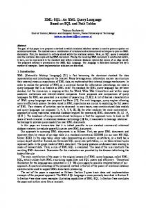
Table 2: Statistics of Index Structures. We also plotted the total query processing cost with the queries type of QT Y P E1 for the three data sets using the strong DataGuide and APEX as minSup varied from 0.002 to 0.05 in Figure 12. We also showed the cost for APEX0 because it represents the upper bound of the cost as we increase minSup. Note that the required path set becomes a set of paths with the length of one when we increase the minSup to high values. Obviously, the query processing cost using APEX0 should be most slow among APEX variants since we need to perform joins of extents for the path expression of the queries with the size of at least two. Therefore, the query processing pays severe performance penalty and it was illustrated by the graphs for all experimental results. Note that the query processing of the strong DataGuide is more inefficient than APEX0 for moderate or high irregular
Play
500 450 400 time(seconds)
350 300 250 200 150 100 50 0 APEX0
SDG
0.002
0.005
0.01
0.03
0.05
0.01
0.03
0.05
0.03
0.05
minSup
(a) Play
FlixML
900 800
time(seconds)
700 600 500 400 300 200 100 0 APEX0
SDG
0.002
0.005 minSup
(b) FlixML
GedML
1600 1400
time(seconds)
1200 1000 800 600 400 200
As minSup decreases, the number of frequently used paths increases and more entries is stored in the HAP EX . Thus, more queries can be directly obtained by look-up of HAP EX . Even though the sizes of the graph structures of the strong DataGuide and APEX are similar for the data sets with moderate or less irregular structure (Play data and FlixML data) given the minSup of 0.002 and 0.005 as shown in Table 2, the query processing cost of APEX is cheaper than that of the strong DataGuide. This is because query results can be directly obtained by the lookup of the hash tree, HAP EX , of APEX without traversing the graph structure, GAP EX . APEX is significantly better for the highly irregularly structured XML data (GedML) than strong DataGuide. From the result, we can conclude that APEX shows much better performance as the structure of the XML data gets more complex. As we also explained previously, as the value of minSup increases, the number of frequent paths decreases and it results in APEX that is very close to APEX0 . Thus, the query processing cost suffers. To evaluate QT Y P E2 queries, the query pruning and rewriting technique [11] is applied. To perform query pruning and rewriting, the query processor with strong DataGuide generally traverse the whole index structure several times. However, the query processor with APEX traverses the partial index structure of GAP EX with the label li . This results that the query pruning and rewriting overhead with APEX is less than that of the strong DataGuide. Even though there is query processing overhead to obtain the query result, APEX shows the best performance over the various data sets. Due to the space limitation, we omit the graph of query performance for QT Y P E2. The effectiveness of APEX is determined by minSup. In our experiment, APEX was efficient with the value of minSup ranging between 0.002 and 0.01. When minSup is 0.005, APEX shows the best performance with the query workload we generated over the various XML data.
0 APEX0
SDG
0.002
0.005
0.01
minSup
(c) GedML Figure 12: Execution times
structure (FlixML and GedML). The query processing time of APEX0 for the GedML is about 1500 seconds and that of the strong DataGuide is about 27000 seconds. The inefficiency of strong DataGuides comes from the fact that its size generated for the XML documents with a complex structure becomes very large. As the Table 2 illustrates, the number of nodes and the number of edges in the strong DataGuide generated for the GedML data are 13392 and 16105 respectively, while they are 78 and 221 in APEX0 produced. Furthermore, to compute a partial matching path query, the query processor should traverse a lot of nodes in the strong DataGuide. While, in APEX, the some queries such as the queries whose length are one can be directly obtained by look-up of HAP EX . This result confirms that the strong DataGuide is generally inefficient for complex XML data. The performance of APEX depends on the value of minSup.
7.
CONCLUSION
In this paper, we propose APEX which is an Adaptive Path indEx for XML data. APEX does not keep all paths starting from the root and utilizes frequently used paths to improve the query performance. In contrast to the traditional indexes such as DataGuides, 1-indexes and the Index Fabric, it is constructed by utilizing the data mining algorithm to summarize paths that appear frequently in query workload. APEX can be incrementally updated in order to minimize the overhead of construction whenever the query workload changes. APEX also guarantees all paths of length two so that any label path expression can be evaluated by joins of extents in APEX without scanning original data. To support efficient query processing, APEX consists of two structures: the graph structure GAP EX and the hash tree HAP EX . GAP EX represents the structural summary of XML data with extents. HAP EX keeps the information for frequently used paths and their corresponding nodes in GAP EX . Given a query, we use HAP EX to locate the nodes of GAP EX that have extents required to evaluate the query. We implemented our APEX and conducted an extensive experimental study with both real-life and synthetic data sets. Experimental results show that APEX improves query processing cost typically 2 to 54 times better than the traditional indexes, with the performance gap increasing with irregularity of XML data.
8.
ACKNOWLEDGMENTS
This work was supported by the Brain Korea 21 Project. Without the support of Yesook Shim, it would have been impossible to complete this work.
9.
REFERENCES
[1] S. Abiteboul. Quering semi-structured data. In Proceedings of the 6th International Conference on Database Theory, pages 1–18, January 1997. [2] S. Abiteboul, D. Quass, J. McHugh, J. Widom, and J. L. Wiener. The lorel query languages for semistructured data. International Journal on Digital Libraries, 1(1):68–88, 1997. [3] R. Agrawal and R. Srikant. Mining sequential patterns. In Proceedings of the 11th International Conference on Data Engineering, pages 3–14, March 1995. [4] S. Boag, D. Chamberlin, M. Fernandez, D. Florescu, J. Robie, J. Simeon, and M. Stefanescu. XQuery 1.0: An XML query language. Working Draft, http://www.w3.org/TR/2001/WD-xquery-20011220, 20 December 2001. [5] P. Buneman, S. B. Davidson, M. F. Fernandez, and D. Suciu. Adding structure to unstructed data. In Proceedings of the 6th International Conference on Database Theory, pages 336–350, January 1997. [6] P. Buneman, S. B. Davidson, G. G. Hillebrand, and D. Suciu. A query language and optimization techniques for unstructured data. In Proceedings of the 1996 ACM SIGMOD International Conference on Management of Data, pages 505–516, June 1996. [7] J. Clark and S. DeRose. XML path language(XPath) version 1.0. W3C Recommendation, http://www.w3.org/TR/xpath, November 1999. [8] B. Cooper, N. Sample, M. J. Franklin, G. R. Hjaltason, and M. Shadmon. A fast index for semistructured data. In Proceedings of 27th International Conference on Very Large Data Bases, January 2001. [9] R. Cover. The XML cover pages. http://www.oasis-open.org/cover/xml.html, 2001. [10] M. F. Fernandez, D. Florescu, A. Y. Levy, and D. Suciu. A query lanaguage for a web-site management system. ACM SIGMOD Record, 26(3):4–11, 1997. [11] M. F. Fernandez and D. Suciu. Optimizing regular path expressions using graph schemas. In Proceedings of the 14th International Conference on Data Engineering, pages 14–23, February 1998. [12] M. N. Garofalakis, R. Rastogi, and K. Shim. SPIRIT: Sequential pattern mining with regular expression constraints. In Proceedings of 25th International Conference on Very Large Data Bases, pages 223–234, September 1999. [13] R. Goldman and J. Widom. DataGuides: Enable query formulation and optimization in semistructured databases. In Proceedings of 23rd International Conference on Very Large Data Bases, pages 436–445, August 1997. [14] J. E. Hopcraft and J. D. Ullman. Introduction to Automata Theory, Language, and Computation.
[15]
[16]
[17]
[18]
[19]
[20]
[21]
[22]
Addison-Wesley Publishing Company, Reading, Massachusetts, 1979. A. Kemper and G. Moerkotte. Access support relations: An indexing method for object bases. Information Systems, 17(2):117–145, 1992. Q. Li and B. Moon. Indexing and querying XML data for regular path expressions. In Proceedings of 27th International Conference on Very Large Data Bases, pages 361–370, September 2001. J. McHugh and J. Widom. Compile-time path expansion in lore. In Proceedings of the Workshop on Query Processing for Semistructured Data and Non-Standard Data Formats, 1999. T. Milo and D. Suciu. Index structures for path expression. In Proceedings of 7th International Conference on Database Theory, pages 277–295, January 1999. S. Nestorov, J. D. Ullman, J. L. Wiener, and S. S. Chawathe. Representative Objects: Concise representations of semistructured, hierarchial data. In Proceedings of the 13th International Conference on Data Engineering, pages 79–90, April 1997. R. T. Ng, L. V. S. Lakshmanan, J. Han, and A. Pang. Exploratory mining and pruning optimizations of constrained association rules. In Proceedings of the 1998 ACM SIGMOD International Conference on Management of Data, pages 13–24, June 1998. Y. Papakonstantinou, H. Garcia-Molina, and J. Widom. Object exchange across heterogeneous information source. In Proceedings of the 11th International Conference on Data Engineering, pages 251–260, March 1995. C. Zhang, J. F. Naughton, D. J. DeWitt, Q. Luo, and G. M. Lohman. On supporting containment queries in relational database management systems. In Proceedings of the 2001 ACM SIGMOD International Conference on Management of Data, May 2001.