application of adaptive neuro-fuzzy inference system in interest rates

Eleftherios Giovanis / Indian Journal of Computer Science and Engineering (IJCSE)

APPLICATION OF ADAPTIVE NEURO-FUZZY INFERENCE SYSTEM IN INTEREST RATES EFFECTS ON STOCK RETURNS ELEFTHERIOS GIOVANIS* Department of Economics, Royal Holloway University of London Egham, Surrey, TW20 0EX, United Kingdom* [email protected] http://www.rhul.ac.uk

Abstract In the current study we examine the effects of interest rate changes on common stock returns of Greek banking sector. We examine the Generalized Autoregressive Heteroskedasticity (GARCH) process and an Adaptive Neuro-Fuzzy Inference System (ANFIS). The conclusions of our findings are that the changes of interest rates, based on GARCH model, are insignificant on common stock returns during the period we examine. On the other hand, with ANFIS we can get the rules and in each case we can have positive or negative effects depending on the conditions and the firing rules of inputs, which information is not possible to be retrieved with the traditional econometric modelling. Furthermore we examine the forecasting performance of both models and we conclude that ANFIS outperforms GARCH model in both in-sample and out-of-sample periods.

Keywords: ANFIS, Interest rates, Stock returns 1. Introduction The issue of interest rate sensitivity remains empirically unresolved. Most of the studies use a variety of shortterm and long-term bond returns as the interest rate factor without providing any rationale for their use. Yet, there is no consensus on the choice of the interest rate factor that should be used in testing the two-factor model. There is a broad consensus among the practitioners and academics that interest rates have a significant effect on share prices, but also there is a little agreement as to whether or not interest rates affect the stock returns. The problem with econometrics is that are based on probabilities and statistics and not on possibilities and membership. To be specific it impossible to find insignificant estimated coefficients over a specific period we examine and therefore we conclude that the phenomenon we examine is rejected, in our cases the effects of interest rates changes on stock returns. This is not absolute logical and correct because traditional econometrics are not able to capture imprecision and non linearities. With fuzzy logic we can retrieve the rules when a specific condition is fired, so there will be always positive and negative effects, in our case, based on specific rules and behaviour of inputs. For example with conventional econometric modelling we can find that there are not significant effects in a specific period, but there are in a sub-period. And the question is how can we find this period? Even if we apply rolling regressions this is not very helpful for financial practical purposes. Additionally, conventional econometric modelling is based on statistical properties, where a long sample is needed. Also, misspecification errors, heteroskedasticity, ARCH effects and autocorrelation in residuals are some problems of econometric estimations. With fuzzy logic and neural networks we can take all the inputs and examine their importance weight in the determination of the output with short or long sample as long as fuzzy rules have been defined. Furthermore, neuro-fuzzy modelling, because it is not based on statistical and econometric properties, autocorrelation and heteroskedasticity in residuals, among other problems, are not examined as the disturbance term is not included in fuzzy regressions and neuro-fuzzy system therefore these problems have no meaning. A proposal for further research study and applications is to introduce the disturbance term in fuzzy and neuro-fuzzy modelling. Additionally, neural networks have been criticized that are black boxes but are able to describe very well the nonlinearities. On the other hand fuzzy logic is not always able to describe nonlinearities appropriately, but is the most efficient method to approach imprecision, and especially in finance, because is determined by human behaviour and this is exactly the true imprecision. More specifically, econometric methodology treats human behavior as a computer based on binary logic with only two possible values, true or false, yes or no, expansive or recessive. To be correct the real values that a human expresses are maybe true, maybe false, or true if and false if. For this reason we use Neuro-Fuzzy system and we believe that is the future in economics and econometrics, as artificial intelligence procedures are already used in finance.

ISSN : 0976-5166

Vol. 2 No. 1

124

Eleftherios Giovanis / Indian Journal of Computer Science and Engineering (IJCSE)

The structure of the paper has as follows: In section 2 we present a short literature review, in section 3 we present the methodology for the GARCH process and the two-index factor model, as also the methodology of ANFIS is described. In section 4 we present the period examined and we describe the data frequency, while in section 5 we present the empirical results and we discuss about them. Finally, in the final section we report our concluding remarks of our findings.

2. Literature Review There is a great number of research studies examining the effects of interest rate changes on stock prices and not returns. Fama [1981] documents a strong positive correlation between common stock returns and real economic variables like capital expenditures, industrial production, real GNP, money supply, lagged inflation and interest rates. Hardouvelis [1987] points out that an inverse relationship between stock prices and changes of interest rate exists and this can be rationalized in terms of money supply surprises. Chen et al. [1999] examine the effect of discount rate changes on the volatility of stock prices and on trading volume and they found that unexpected discount rate changes contributed to higher, though short-lived, volatility and trading volume. Stock returns sensitivity to interest rates was theoretically advocated by Merton [1973], Long [1974] and Stone [1974]. Essentially, risk averse investors demand higher compensation for exposure to factors, other than the market portfolio, that are correlated with intertemporal changes in the investment opportunity set. Stone [1974] has offered another means of expanding the market model. He has proposed a two-index model consisting of the traditional equity market index and a debt market index and he justified the model by arguing that individual equity securities exhibit varying degrees of sensitivity to interest rates and that the opportunity to invest in risky debt securities may represent an attractive alternative to riskless assets and risky equity securities. Booth and Officer [1985] and Bae [1990] test the effect of current and unanticipated changes in interest rate. Fraser et al., [2002[ examine the effect of unanticipated rate changes. All these studies, as also other research empirical evidences [Fama and Schwert (1977); Christie, (1981)], found strong support for a negative effect of both current and unanticipated interest changes on bank stock returns. While some studies have found the interest rate factor to be an important determinant of common stock returns of banks, on the contrast Chance and Lane [1980] have found the returns to be insensitive or other supporting that stock returns only marginally explained by the interest rate factor, so these studies find no incremental explanatory power for interest rate changes [Lloyd and Shick, 1977)]. Research studies employing fuzzy logic, ANFIS and generally artificial intelligence procedures have not yet been made.

3. Methodology 3.1 Two factor model The proposed generalized formulation of the two-factor model [Stone, (1974)] is as follows:

R pit   i 0   i1 Rmt   i 2 ΔI t   it

(1)

, where

i0

is the constant

R pit denotes the weekly returns of an equally weighted portfolio i of stock in week t, Rmt is the weekly return on the market portfolio in week t, ΔIt is a default free debt index as proxy of interest rates in period t,

 it

is a stationary y stochastic process with zero mean for each portfolio i,

ISSN : 0976-5166

Vol. 2 No. 1

125

Eleftherios Giovanis / Indian Journal of Computer Science and Engineering (IJCSE)

The one month , three, six and twelve months Treasury bill rates have been tested as the interest rate variable in equation (1), but we present randomly only the results for three months Treasury bill rates because the conclusions are the same in all cases and there is no difference using short-term or longer-term interest rates. Because with ordinary least squares we found autocorrelation and ARCH effects we estimate with symmetric GARCH (p,q) process, which is mainly used in financial econometric literature. GARCH model was proposed by Bollerslev [1986]. The mean equation remains the same as in equation (1) but GARCH (1,1) process is:

 it ~ (0,  2 )

(2)

t

, where



2 t

  0   1u t 1   2 t 1 2

2

(3)

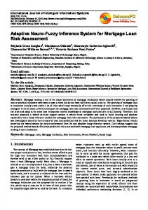
Additionally we have tested asymmetric GARCH models [Nelson, (1991); Glosten et al., (1993)] but the results are not presented, as are exactly the same with those of symmetric GARCH process. 3.2 Adaptive Neuro-Fuzzy Iinference System (ANFIS) We follow a simple ANFIS system in order to improve its forecasting performance and to make it much more useful. We incorporate two linguistic terms {positive, negative}. More linguistic terms can be introduced, as very positive and very negative, but the forecasting performance is almost the same, indicating that we can simplify the procedure by taking less linguistic terms and less rules. On the other hand more linguistic terms might be more useful, but in the case we examine financial professionals and traders are interesting mainly on positive and negative returns. The rules are 4 because we have two inputs with two linguistic terms and it is 2*2=4. These rules are: IF RET is negative AND IR is negative THEN f1=p1x1 + q1x2 + r1 IF RET is negative AND IR is positive THEN f2=p2x1 + q2x2 + r2 IF RET is positive AND IR is negative THEN f3=p3x1 + q3x2 + r3 IF RET is positive AND IR is positive THEN f4=p4x1 + q4x2 + r4 , where RET denotes the General stock index returns and IR denotes the interest rate changes. We choose the AND operator so we will take the product instead to min operator to avoid monotonic results. Also each rule has 2 parameters plus the constant hence there will be 3*4=12 parameters. Jang [1993] and Jang and Sun [1995] introduced the adaptive network-based fuzzy inference system (ANFIS). This system makes use of a hybrid learning rule to optimize the fuzzy system parameters of a first order Sugeno system. An example of a two input with two rules first order Sugeno system can be graphically represented by Fig. 1.

Fig. 1 Example of ANFIS architecture for a two-input, two-rule first-order Sugeno model

ISSN : 0976-5166

Vol. 2 No. 1

126

Eleftherios Giovanis / Indian Journal of Computer Science and Engineering (IJCSE)

, where the consequence parameters p, q, and r of the nth rule contribute through a first order polynomial of the form: (4) f n  p n x1  q n x 2  rn The ANFIS architecture is consisted of two trainable parameter sets, the antecedent membership function parameters and the polynomial consequent parameters p,q,r. The ANFIS training paradigm uses a gradient descent algorithm to optimize the antecedent parameters and a least squares algorithm to solve for the consequent parameters. Because it uses two very different algorithms to reduce the error, the training rule is called a hybrid. The consequent parameters are updated first using a least squares algorithm and the antecedent parameters are then updated by backpropagating the errors that still exist. The ANFIS architecture consists of five layers with the output of the nodes in each respective layer represented by Oil, where i is the ith node of layer l. Because we have four rules and two inputs in the case we examine the steps for ANFIS system computation are: In the first layer we generate the membership grades

Oi   1

Ai

( x 1 ),  B i ( x 2 )

(5)

, where x1 and x2 are the inputs. In layer 2 we generate the firing strengths or weights

Oi  wi   j 1 (  Ai ( x1 ),  Bi ( x2 ))  andmethod (  Ai ( x1 ),  Bi ( x 2 )) 2

m

 product (  Ai ( x1 )   Bi ( x2 ))

(6)

In layer 2 we use the AND relation, as it was mentioned previously, so we take the product operator. In layer 3 we normalize the firing strengths and it will be: 3

Oi  wi 

wi w1  w2  w3  w4

(7)

, where i is for i=1,2,3,4. In layer 4 we calculate rule outputs based on the consequent parameters. 4

O i  y i  w i f i  w i ( p i x1  q i x 2  ri ) In layer 5 we take 5

Oi 

 i

wi f i 

w f w i

(8)

(9)

i

i

i

In the last layer the consequent parameters can be solved for using a least square algorithm as:

Y  X 

(10)

, where X is the matrix

X  [ w1 x  w1  w2 x  w2  ...  w9 x  w9 ]

(11)

and θ is a vector of unknown parameters as:

   p1 , q1 , r1 , p 2 , q 2 , r2 , ,..., p 9 , q 9 , r9 T

(12)

, where T indicates the transpose. Because the normal least square method leads to singular inverted matrix we use the Singular Value Decomposition (SVD) with Moore-Penrose pseudoinverse of matrix [Moore, (1920); Penrose, (1955); Petrou and Bosdogianni, (2000)]. Other methods that can be used to eliminate the particular problem is Lower Triangular, Upper Triangular and Orthogonal decomposition (QR) among others. More specifically the Singular Value Decomposition (SVD) procedure is:

X  USV

ISSN : 0976-5166

Vol. 2 No. 1

T

(13)

127

Eleftherios Giovanis / Indian Journal of Computer Science and Engineering (IJCSE)

The singular values in S are positive and arranged in decreasing order. Their magnitude is related to the information content of the columns of U -principle components- that span X. Therefore, to remove the noise effects on the solution of the weight matrix, we simply remove the columns of U that correspond to small diagonal values in S. The weight matrix is then solved for using the following:

  VS

1

U TY

(14)

For the first layer and relation (5) we use the Triangular, Gaussian and sigmoidal shape membership functions. We have described the computation procedure for the consequent parameters by using least squares algorithm with Moore-Penrose pseudoinverse matrix. The next step is to describe the training procedure for the antecedent parameters with the error backpropagation algorithm and the simple steepest descent method [Tsoukalas and Uhrig, (1996); Denai et al., (2004); Khan et al., (2010)]. The triangular function is defined as:

 x j  a ij b  , if x j  a ij  ij  1  (15)  ij ( x j ; a ij , b ij )   b ij / 2 2     0 , otherwise  , where αij is the peak or center parameter and bij is the spread or support parameter. The symmetrical Gaussian membership function is defined as:

 ij ( x j ; c ij , 

ij

 ( x j  c ij ) 2 )  exp   2  2 ij 

   

(16)

, where cij is the center parameter and σij is the spread parameter. The last membership function we examine is the Sigmoid shape function such as:

 ij ( x j ; a ij , c ij ) 

1 1  exp(  a ij ( x ij  c ij )

(17)

, where cij locates the center of the curve and aij is the spread parameter. The antecedent parameter c update is:

c ij ( n  1 )  c ij ( n ) 



c

p



E  c ij

(18)

,where ηc is the learning rate for the parameter cij, p is the number of patterns and E is the error function which is:

E 

1 ( y  yt )2 2

(19)

, where yt is the target-actual and y is ANFIS output variable. The chain rule in order to calculate the derivatives used to update the membership function parameters are:

E  E  y  y i  w i   ij      c ij  y  y i  w i   ij  c ij

(20)

The partial derivatives for two inputs are derived below:

E  y  yt  e  y ij

(21)

For the output is:

y 

n



i 1

, hence it will be

ISSN : 0976-5166

yi

y 1 yi

Vol. 2 No. 1

(22)

(23)

128

Eleftherios Giovanis / Indian Journal of Computer Science and Engineering (IJCSE)

yi 

wi n



i 1

( p i x 1  q i x 2  ri )

(24)

wi

, hence it will be :

yi ( pi x1  qi x 2  ri )  y  n wi  wi

(25)

i 1

wi 

m





j 1

, then it will be

(26)

ji

wi wi    ji  ji

(27)

The last partial derivative, Eq. 27 depends on the membership function we examine. The update equations for antecedent cij, and σij parameters of Gaussian function are:

cij (n  1)  cij (n) c  e

( pi x1  qi x2  ri )  y  x ij - cij   ij (x j )   n σ 2 ij   wi

(28)

i 1

2 ( pi x1  qi x2  ri )  y  xij - cij   ij (n 1) ij (n) σ  e  (x )  n  σ3ij  i j   wi

(29)

i1

The update equations for aij are, bij are respectively

ij (n 1)  ij (n) α  e

( pi x  ri )  y n

w

i

i 1

bij (n 1)  bij (n) b  e

( pi x  ri )  y n

w i 1

i



wi 2 xj  aij  ij (xj ) bij

(30)

wi 1 ij (xj )  ij (xj ) bij

(31)



In a similar fashion the update equations for sigmoidal shape fuzzy membership function can be derived. The next step is to define the initial values for antecedent parameters. In all cases we get as initial values for enter and bases parameters the mean and standard deviation. To be specific we get one sample where the returns on assets are negative and one sample where the returns are positive. The same procedure is followed for cash flow. So for center parameters a, c and c of triangle, Gaussian and sigmoid respectively we take the average for negative and positive samples. On the other hand for the base parameters, b, σ and a we take the standard deviations of the respective samples. For the center and consequent RHS parameters we set up the value 0.05 as the learning rate and for base parameters we set up the learning rates at 0.01. 4. Data The sample period we examine in the current study is 2003-2009. We examine 15 Greek banks and the data are on weekly frequency. Additionally, the period 2003-2008 is used as the in-sample or training data period and the remaining period 2009 is used as the out-of-sample or testing data period. The notion of portfolio theory and

ISSN : 0976-5166

Vol. 2 No. 1

129

Eleftherios Giovanis / Indian Journal of Computer Science and Engineering (IJCSE)

systematic risk was not developed at that time, and it was until later when Stone [1972] extended the market model by incorporating the effects of debt indices. To assess the effect of the market yield so we have constructed equally weighted stock portfolios for the following sectors the Greek The General index of Athens stock market is used as proxy for the Greek banks, while the Libor of one and three months is used as the interest variable in equation (1). Additionally, we examine if the equally weighted portfolios returns, the General index of Athens stock exchange market returns and interest rate changes are stationary. To be specific we confirm this assumption by applying Augmented Dickey-Fuller-ADF [Dickey and Fuller, (1979)] unit root test and KPSS stationary test [Kwiatkowski et al., (1992)]. The ADF test is defined from the following relation:

 y t    γ y t 1   1  y t 1  ....   p  y t  p   t   t

(32)

, where yt is the variable we examine each time. In the right hand of regression (32) the lags of the dependent variable are added with order of lags equal with p. Additionally, regression (32) includes the constant or drift μ and trend parameter β. The disturbance term is defined as εt. In the next step we test the hypotheses: H0: φ=1, β=0 against the alternative hypothesis H1: |φ|