Water Resources Systems—Hydrological Risk, Management and Development (Proceedings of symposium HS02b held during 1UGG2003 at Sapporo, July 2003). IAHS Publ. no. 281, 2003.
107
Application of dynamic-stochastic runoff generation models for estimating extreme flood frequency distributions
L. S. K U C H M E N T , A. N. G E L F A N & V. N. D E M I D O V Water Problems Russia
Institute
of the Russian
Academy
of Sciences,
3 Gubkina
Str., 119991
Moscow,
[email protected]
Abstract A physically based model of runoff generation is coupled with Monte Carlo simulations of the model inputs to estimate flood peak frequency distributions. The runoff generation model represents the following hydrological processes: snow cover formation and snowmelt, freezing and thawing of soil, vertical soil moisture transfer and evaporation, overland and channel flow. The Monte Carlo simulations of snowmelt runoff are based on stochastic models of daily precipitation series, daily air temperature and daily air humidity deficit (for continuous simulations during autumn-winter-spring seasons) or statistical distributions of snow water equivalent, depth of frozen soil, and soil moisture content before snowmelt (for simulations only during snowmelt flood events). To simulate the rainfall runoff during a warm period, the statistical disfributions of precipitation volumes, precipitation duration, duration of dry periods, and mean air humidity deficit for dry periods, were used. A case study was carried out for the Seim River basin situated in the southwestern part of Russia. The dynamic-stochastic models developed were applied for estimating changes in the exceedence probabilities of runoff characteristics for three land-use scenarios. Uncertainties in estimating flood characteristics caused by errors in model parameters have been investigated. Key words Monte Carlo simulation; physically based modelling; rainfall flood; Seim River, southwest Russia; snowmelt flood; stochastic modelling
INTRODUCTION
Increasing demands for acceptable risk in water resources management is a motivation for improving methods of estimating possible flood events of very low probabilities. At the same time, frequency analyses of measured flood peaks are becoming more difficult because of the short length of measured flood peak series or man-induced nonstationarity of these series. As a result, the idea of deriving flood frequency distributions from meteorological series, which are usually longer and less affected by human activity than the hydrological series, is becoming more and more attractive. It seems that Velikanov (1949) first used the idea of determining the probability of the logarithm of snowmelt flood peaks as a product of the probabilities of the logarithms of the maximum snow water equivalent and the duration of snowmelt. Eagleson (1972) was the first to derive flood frequency distributions from the statistical characteristics of rainfall but he implemented a simplistic description of runoff generation processes. The development of Eagleson's analytical method and its application to deriving peak frequencies of rainfall and snowmelt floods are described by Carlson & Fox (1976), Hebson & Wood (1982), Diaz-Granados et al. (1984) and many others.
108
L. S. Kuchment et al.
The numerical solution of the differential equations describing runoff generation processes was combined with the simulation of meteorological inputs by the Monte Carlo method by Kuchment & Gelfan (1991). This method facilitates application of complicated nonlinear models of runoff generation and complex stochastic models of meteorological inputs. While Kuchment & Gelfan (1991), because of computer time limitations, applied relatively simple models, Calver & Lamb (1995), Salmon et al. (1997), Cattanach et al. (1997), Hashemy et al. (2000), Cameron et al. (2000) and Kuchment & Gelfan (2002) used more elaborate methods. In this paper, the methodology developed in Kuchment & Gelfan (2002) is applied to estimate flood peak frequency distributions for floods of mixed snowmelt-rainfall origin. The paper also presents results of numerical experiments determining the sensitivity of exceedence probabilities of runoff characteristics to land-use change and analyses of uncertainty, both for continuous simulations of the flood series and the event flood approach.
THE STUDY SITE AND THE PHYSICALLY BASED MODEL OF FLOOD GENERATION 2
The Seim River basin (the catchment area at Kursk is 7460 km ) is a part of the Dnieper River basin. The basin relief is a rugged plain with many river valleys, ravines and gullies. The soils are mainly chernozem, grey forest soil, and meadow soil. The groundwater level fluctuates at 15-20 m below the land surface. The greater part of the basin (-70%) is ploughed, the forest occupies about 10% of the basin area; pastures and urbanized areas occupy about 20%. Mean annual precipitation is 550-600 mm, the mean snow water equivalent before melting is 85 mm. The mean snowmelt runoff is 55 mm; the mean annual peak discharge is 592 m s" ; their coefficients of variation are 0.43 and 0.81, respectively. The mean snowmelt peak discharge is almost 20 times higher than the rainfall one. However, rainfall can play an essential role in the formation of the spring flood peak discharge. Overland flow is the main mechanism of snowmelt runoff generation for the Seim River basin. The subsurface contribution to total runoff during flood periods is negligible. Rainfall runoff usually occurs during the summer-autumn period only on small areas located near river channels. The runoff coefficients of most rainfall floods are about 0.05. The model of runoff generation used here is based on a finite-element discretization of the river basin and includes description of the following hydrological processes: snow cover formation and snowmelt, freezing and thawing of the soil, vertical soil moisture transfer and evaporation, overland and channel flow. After analysis of hydrometeorological data and numerical experiments, the following structure of the runoff generation model for the basin was chosen. To represent the snowpack, vertically averaged equations of snow processes at a point were applied (Kuchment & Gelfan, 1996; Kuchment et al, 2000). These include the description of the temporal change of the snow depth, content of ice and liquid water, snow density, snowmelt, sublimation, melt water re-freezing and snow metamorphism. The equations describing soil freezing and thawing include descriptions of heat transfer in the snow, movement of the soil freezing front, and soil moisture transfer from the unfrozen soil layer to the freezing front (Kuchment, 1980; Kuchment & 3
1
Dynamic-stochastic
runoff generation models for extreme flood frequency
distributions
109
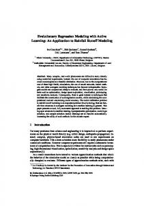
Gelfan, 1993). Changes in the unfrozen soil moisture content and infiltration into the soil during the warm period were calculated using the Richards equation in the diffusive form. The soil parameters (diffusivity, hydraulic conductivity of unfrozen soil, heat capacities and thermal conductivities of frozen and unfrozen soil) were calculated by empirical formulae (Kuchment et al, 1983; Kuchment et al, 2000). The intensity of infiltration into the frozen soil, evaporation rate, and detention of water by basin storage were calculated using formulae from Kuchment & Gelfan, 2002). It was assumed that the snow water equivalent, and the depth of the frozen soil before snow melt, were gamma-distributed within each finite element. The mean spatial values of these variables were calculated using meteorological data and the coefficients of spatial variation were determined using empirical formulae (Kuchment & Gelfan, 1993). To calculate rainfall runoff losses, it was also assumed that the soil saturated hydraulic conductivity is gamma-distributed (the parameters of these distributions were determined according to Kuchment et al. (1996)). To simulate overland and channel flow, one-dimensional kinematic wave equations were applied (Kuchment et al, 1986). For numerical integration of these equations, the finite element method was used. The finite element discretization of the drainage area was based on the river basin topography, soils, land use and vegetation. To calibrate and verify the model of runoff generation for the basin, daily meteorological data for 20 years (1969-1988) were used. Five parameters were calibrated against the measured runoff hydrographs for the period of 1969-1978. The rest of the parameters was assigned on the basis of the available measurements at four agrometeorological sites within the basin area. The model was verified by comparisons of the measured and calculated hydrographs for the period of 1979-1988 (Fig. 1). As can be seen from Fig. 1, the model gives satisfactory simulations of the Seim River hydrographs.
STOCHASTIC MODELS OF METEOROLOGICAL INPUTS To simulate the meteorological inputs, models of precipitation, daily air temperature for the cold period, and air humidity deficit for the warm period have been developed. For choosing the structure of these models and for fitting the parameters, meteoro logical data from a meteorological station for a period of 101 years (1891, 1892, 18961941, 1943-1995) were used. The model of daily precipitation occurrence throughout the year was represented as a first-order Markov chain with the conditional probability of a dry day after a dry day, and the probability of a dry day after a wet day, equal to 0.7 and 0.4, respectively. Daily precipitation amounts for days with non-zero precipitation were described using the gamma distribution with different parameters for the cold and warm seasons: the mean values are 2.5 mm and 4.7 mm, respectively; the coefficients of variation are 1.52 and 1.40, respectively. In addition, for the warm period, the duration of rainfall was simulated. It was assumed that it is a gamma-distributed variable with a mean of 13 200 s, and a coefficient of variation of 1.02. The correlation between storm duration and volume was taken into account (the coefficient of correlation is 0.67). To estimate the maximum rainfall rate, the hyetograph was represented as an isosceles triangle.
L. S. Kuchment et al.
110
1980
1979
1200 £ ' 900 ]
500
m / s
400 300
L
j
200 100 0
11/9
20/12
15/11
23/2
—n3/6
11/9
20/12
Thus, the Monte Carlo simulation procedure for the precipitation series is as follows: first, the wet-dry day occurrence and daily precipitation amounts for wet days were generated for the whole year; then rainfall durations and hyetographs were generated for every wet day of the warm period. A comparison between simulated and
Dynamic-stochastic
runoff generation models for extreme flood frequency distributions
111
Table 1 Mean seasonal characteristics of precipitation estimated from 101-years of measurements and using simulated series.
Measured Simulated
Precipitation Days with total non-zero (mm) precipitation 1 May-31 October
Days with precipitation >10 mm
Precipitation Days with total non-zero (mm) precipitation 1 November-30 April
Days with precipitation >10mm
347 352
10 9
242 234
4 5
73 76
94 91
measured values of mean seasonal precipitation totals, mean number of days with non zero precipitation and with precipitation more than 10 mm day" is shown in Table 1. Because of the strong autocorrelation in the daily air temperature series, the follow ing approach was applied. At first, the observed sequences of daily air temperature for cold seasons were divided by their average values to obtain the normalized series (fragments) for each season. Then these series were separated into several groups taking into account a range of the average temperature. The distribution of the average seasonal temperature was fitted by a normal probability distribution. For generating synthetic temperature series, a random value of the average seasonal temperature was generated and multiplied by the fragment, randomly chosen from the corresponding group. The histogram of daily air humidity deficit values was fitted by a lognormal distribution. It was assumed that on wet days the humidity deficit was negligible. According to the available data, the cross-dependence between meteorological inputs is negligible so there was no need to take it into account. 1
CONSTRUCTING THE FLOOD FREQUENCY DISTRIBUTION We tested two procedures of simulating possible rainfall-snowmelt flood events. Initially we applied Monte Carlo simulations to construct continuous series of meteorological inputs (a wet-dry days sequence was generated for every year, daily precipitation for wet days, daily air humidity deficit for dry days, and daily air temperature for every cold period from 1 November to 30 April) and these inputs were used to calculate possible spring-summer floods. In the second procedure, we tried to avoid long-term stochastic modelling of meteoro logical inputs before snowmelt. To this end, we first used the available series of meas ured daily air temperature, air humidity deficit, and precipitation for the period from 1 May to 1 March for 34 years in order to calculate the soil moisture content, the depth of the frozen soil, and the snow water equivalent before the beginning of snowmelt for each year. Then the empirical probability distributions of these values were constructed and fitted by gamma-distributions. These distributions were used for the Monte Carlo simulation of different combinations of initial conditions in the river basin before snow melt. Finally, the initial conditions were combined with the Monte Carlo simulations of meteorological inputs during spring-summer periods to obtain the simulated floods. Figure 2(a) shows a comparison of the exceedence probabilities of snowmelt flood peaks calculated from 61-years of data and the exceedence probabilities determined from the 20 000 hydrographs obtained on the basis of synthetic input data. The mean value of snowmelt peak discharge calculated by the first procedure is 619 m s" and 3
1
L. S. Kuchment et al.
112
0.001
0.01
0.1
1
0.01
0.1 Exceetkiuce probability
1
Fig. 2 Exceedence probabilities of snowmelt (a) and rainfall (b) peak discharges of the Seim River. Points: the observed peaks; bold line: calculations using the dynamicstochastic model with random meteorological inputs; thin line: calculations using the dynamic-stochastic model with random initial conditions.
3
1
appears to be closer to the observed mean value (592 m s" ) than the one calculated using the second procedure (644 m s" ). However, the coefficient of variation of flood peaks and the quantiles of low exceedence probabilities calculated using the second procedure are closer to the corresponding values obtained from 61-years of flood data. It appears that the first procedure allows us to reproduce the averaged conditions of snowmelt runoff generation more accurately, but the conditions of extreme floods less accurately. Perhaps, using the second procedure, we can determine more reliably low exceedence probabilities. Simulations of rainfall floods were carried out for the period 1 May to 31 October. Rainfall affects the flood frequency distribution only during snowmelt. The exceed ence probabilities of rainfall flood peak discharges are shown in Fig. 2(b). 3
1
INFLUENCE OF CHANGE IN THE BASIN LAND USE ON THE FLOOD FREQUENCY DISTRIBUTION The model was applied to estimate exceedence probabilities of flood characteristics for three land-use scenarios in the Seim River basin (beginning of the twentieth century, present time, and for future conditions). The main differences in these scenarios are associated with changes in the portion of area of agricultural land and types of land treatment. At the beginning of the last century, all agricultural lands were used as pasture after harvest, and ploughing occurred after grazing. At present, only about 20% of the agricultural land (-70% of the basin area) is used for grazing after harvesting. The forest and virgin land area portions did not change during the last century. However, it is supposed that in the future the virgin lands will be used for agriculture and deep autumn ploughing will be applied to all agricultural lands. Different land uses and land treatment practices result in changes of the saturated hydraulic conductivity and the free storage capacity. The simulation results suggest that the mean value of simulated flood peaks during the twentieth century decreased by about 12%; the coefficient of variation of the peaks increased from 0.77 to 0.84. The ploughing of the present virgin lands can decrease the present-day mean flood peak from 644 m s" to 554 m s" . However, the coefficient of variation of flood peaks will change insignifi3
3
1
1
Dynamic-stochastic
runoffgeneration
models for extreme flood frequency distributions
113
cantly. As a result, the flood peak discharges of low exceedance probabilities will change less than the peaks of small and moderate floods ANALYSIS OF UNCERTAINTY DUE TO ERRORS IN THE MODEL PARAMETERS Advantages of constructing flood frequency distributions by dynamic-stochastic simul ations may be significantly constrained by the uncertainty in the simulation process. Sources of uncertainty include inappropriate model structure, errors in the data and errors in the calibrated model parameters. We tried to estimate only the uncertainty caused by errors in assigning the parameters, considering this source as the most important one. The numerical experiments showed that the mean value and the coefficient of variation of the peak discharges are most sensitive to three parameters: (1) the saturated hydraulic conductivity, K , (2) the Manning's roughness coefficient for the river channels, n , and (3) a coefficient p in the relationship between degree-day factor and snow density. Analyses of measurements of saturated hydraulic conductivity for the main basin soil types have shown that the value of K can vary from 0.0005 to 0.004 m s" . According to our experience with kinematic wave models for different river channels, the value of n can vary within a range of 0.02-0.1 s m~ . Finally, the ranee of possible changes of the value of p was set to 1.2 x 1 0 " - 4.2 x 10'' ' V ^ C ' k g ' s" on the basis of available measurements of snowmelt rates in the forested-steppe zone. Assuming parameters K , n and P to be statistically independent and uniformly distributed over the assigned intervals, we generated 200 combinations of these parameters and calculated 10 000 hydrographs for each combination using the dynamic-stochastic model. The exceedence probabilities of annual maximum discharges calculated by these 200 samples, the 95% confidence limits of the exceedence probabilities, and the exceedance probabilities of the observed discharges are shown in Fig. 3(a). The figure indicates that the variations in the model parameters result in significant uncertainty of the quantiles of low exceedence probability. For example, the 95% confidence limits for Qmax of 0.001 probability vary from 2000 to 3700 m s" ; for Qmax of 0.01 probability these limits vary from 1500 to 2900 m s" . However, as can be seen from Fig. 3(b), these confidence intervals are significantly s
c
1
s
1/3
c
10
s
3
1
1
1
c
3
1
Fig. 3 95% confidence intervals calculated (a) for the snowmelt flood frequency curve derived from the dynamic-stochastic model, and (b) for the log Pearson-type III frequency curve fitted to the observed 61-year data series.
114
L. S. Kuchment et al.
narrower than the ones obtained (Guidelines, 1982) for the log Pearson-type III frequency curve fitted to the observed 61-year data series.
CONCLUSIONS Monte Carlo simulations of runoff hydrographs based on a physically based model of runoff generation and a stochastic model of meteorological inputs can give more reliable statistical distributions of runoff characteristics than the statistical analysis of short observed runoff series. This methodology can be successfully applied to estimate the change of flood characteristics resulting from a change in land use. For further improvements of this technology, it is necessary to investigate the predictive uncertainty caused by errors in the input data and in the model structure. This uncertainty can vary within a wide range. Acknowledgement The present work was carried out as a part of the research project supported by the Russian Foundation for Basic Research (Grant no. 02-05-65009). REFERENCES Calver, A. & L a m b , R. (1995) Flood frequency estimation using continuous rainfall-runoff modelling. Phys. Chem. 20, 479^183.
Earth.
C a m e r o n , D. S., Beven, K. J. & N a d e n , P. (2000) Flood frequency estimation by continuous simulation under climate c h a n g e (with uncertainty). Plydrol. Earth System Sci. 4 , 3 9 3 - 4 0 6 . Carlson, R. F. & Fox, P. (1976) A northern snowmelt-flood frequency m o d e l . Water Resour.
Res. 1 2 , 7 8 6 - 7 9 4 .
Cattanach, J. D., Chin, W. Q. & Salmon, G. M. (1997) Estimating the m a g n i t u d e and probability of extreme events, Hydropower97
July 1997. T r o n d h e i m , N o r w a y .
D i a z - G r a n a d o s , M. A., V a l d e s , J. B . & Bras, R. L. ( 1 9 8 4 ) A physically based flood frequency distribution. Water Resour. Res. 2 0 , 9 9 5 - 1 0 0 2 . H a s h e m i , A. M., Franchini, M. & O ' C o n n e l l , P. E. (2000) Climatic and basin factors affecting the flood frequency curve. Hydrol.
Earth System Sci. 4 , 4 6 3 ^ 1 9 8 .
Eagleson, P. S. ( 1 9 7 2 ) D y n a m i c s of flood frequency. Water Resour.
Res. 6 , 8 7 8 - 8 9 8 .
Guidelines ( 1 9 8 2 ) Guidelines for Determining Flood Flow Frequency. Bulletin no. 17 of the Hydrology S u b c o m m i t t e e of the Interagency A d v i s o r y C o m m i t t e e on Water Data. US D e p a r t m e n t of the Interior Geological Survey, Office of W a t e r Data Coordination, Reston, Virginia, U S A . H e b s o n , C. & W o o d , E. F. ( 1982) A derived flood frequency distribution. Water Resour.
Res. 1 8 , 1 5 0 9 - 1 5 IS.
K u c h m e n t , L. S. ( 1 9 8 0 ) M o d e l s of the river runoff generation processes. H y d r o m e t e o i z d a t , Leningrad (in Russian). Kuchment, L. S. & Gelfan, A. N . (1991) Dynamic-stochastic models of rainfall and snowmelt runoff. Hydrol. Sci. J. 3 6 , 1 5 3 - 1 6 9 . Kuchment, L. S. & Gelfan, A. N . (1993) Dynamic-stochastic models of river runoff generation. N a u k a , M o s c o w (in Russian). Kuchment, L. S. & Gelfan, A. N . (1996) T h e determination of the s n o w m e l t rate and mellwater outflow from a s n o w p a c k for modelling river runoff generation. J. Hydrol.
179, 2 3 - 3 6 .
Kuchment, L. S. & Gelfan, A. N . (2002) Estimation of extreme flood characteristics using physically based models of runoff generation and stochastic meteorological inputs. Water International
27(1), 77-86.
K u c h m e n t , L. S., D e m i d o v , V. N . & Motovilov, Yu G. ( 1 9 8 3 ) River runoff formation (physically-based m o d e l s ) . N a u k a , M o s c o w (in Russian). K u c h m e n t , L. S, D e m i d o v , V. N . & Motovilov, Y . G . ( 1 9 8 6 ) A physically based model of the formation of s n o w m e l t and rainfall runoff. In: Symposium on the Modeling Snowmell-lndtteedProcesses (Budapest), 2 7 - 3 6 . I A H S Publ. no. 155. Kuchment, L. S., D e m i d o v V. N . , N a d e n P. S., C o o p e r D. M., Broadhurst P. (1996) Rainfall-runoff m o d e l i n g of the O u s e basin, North Yorkshire: an application of a physically based distributed model. J. Hydrol 1 8 1 , 3 2 3 - 3 4 2 . K u c h m e n t , L. S, Gelfan, A. N , D e m i d o v , V. N . ( 2 0 0 0 ) A distributed model of runoff generation in the permafrost regions. J. Hydrol. 2 4 0 , 1-22. S a l m o n G. M . , Chin, W. Q. & Plesa V. (1997) Hydropower97, 1-8. T r o n d h e i m , "Norway
Estimating the m a g n i t u d e and probability of extreme
floods.
Velikanov, M. A. (1949) T h e composition m e t h o d to estimate e x c e e d a n c e probabilities of s n o w m e l t flood peak discharges. Meteorology and Hydrology^, 6 1 - 6 7 (in Russian).