Scientific Research and Essays Vol. 5(22), pp. 3384-3397, 18 November, 2010 Available online at http://www.academicjournals.org/SRE ISSN 1992-2248 ©2010 Academic Journals
Full Length Research Paper
Application of Fuzzy mathematical programming approach to the aggregate production/distribution planning in a supply chain network problem T. Paksoy1, N. Y. Pehlivan2 and E. Ozceylan1* 1
Department of Industrial Engineering, Selçuk University, Campus 42031, Konya, Turkey. 2 Department of Statistics, Selçuk University, Campus 42031, Konya, Turkey. Accepted 6 July, 2010
This paper presented an application of Fuzzy mathematical programming model to solve network design problems for supply chains via considering aggregate production planning (APP). APP goals to minimize all costs through optimal levels of production, subcontracting, inventory, backorder and work levels over a time period to meet the demand. Fuzzy logic was applied to solve the uncertain production/distribution/subcontracting costs and capacities. However, most of the existing models deal the APP problems without integrating supply chain networks. In our model, APP and supply chain design problem were considered within a single plan horizon to get better managerial results. A supply chain network which includes suppliers, manufacturers, subcontracts, retailers and customers, was developed to illustrate the performance of the proposed model. A numerical example was presented to clarify the features proposed approach. In applying the model, decision makers should find a potential to represent their human resources policies regarding the overtime and subcontract production under material requirements constraints. Key words: Supply chain network optimization, aggregate production planning, material requirements constraint, triangular Fuzzy numbers, possibilistic linear programming. INTRODUCTION Supply Chain Management (SCM) has received considerable attention from academicians and practitioners during the last several decades. Design and optimization of strategic production/distribution models for SCM is one of the most popular problems in this research field. Generally, the problem is defined with following entities: (i) location of facilities (plants, retailers, suppliers, etc.) to be opened; (ii) design of the network configuration; (iii) satisfy customer’s demand with minimization of the total cost including purchasing cost, transportation cost, fixed operating cost, etc. (Paksoy et al., 2007). The proposed APP model attempts to minimize total costs which are, transportation costs, production costs,
*Corresponding author. E-mail:
[email protected]. Tel: +90 332 223 20 75. Fax: +90 332 241 06 35.
inventory and backorder costs, labor hiring and firing costs in terms of inventory and backorder levels, work force level, subcontract and manufacturer production levels, regular time and overtime production levels, labor hiring and firing levels, demands and transportation capacities. This model simultaneously minimizes the most possible value of the imprecise total costs, maximizes the possibility of obtaining lower total costs and minimizes the risk of obtaining higher total costs. This study is organized as follows: After the introduction, where the literature research and aim of the study are described, the developed Fuzzy linear programming model is presented with its indices, parameters and objective function. The study further illustrates the working principle of the approach on a numerical example and discusses the results of the numerical example by LINDO 6.1 package program, after which the entire study is concluded.
Paksoy et al.
Literature review In this field, numerous researches were conducted. Williams (1981) developed seven heuristic algorithms to minimize distribution and production costs in supply chain. Cohen and Lee (1989) presented a deterministic, mixed integer, non-linear programming with economic order quantity technique to develop global supply chain plan. Pyke and Cohen (1993) developed a mathematical programming model by using stochastic sub-models to design an integrated supply chain which involves manufacturers, warehouses and retailers. Syarif et al. (2002) tried to design a supply chain distribution network under capacity constraints in each echelon by a new algorithm based genetic algorithm. Yan et al. (2003) proposed a strategic model for supply chain network design under material requirements and logic constraints. Their model which consists of a network involves suppliers, manufacturers, distribution centers and customers, has a mixed integer structure. Yılmaz (2004) handled a strategic planning problem for three echelon supply chain involving suppliers, manufacturers and distribution centers to minimize transportation, distribution and production costs. Gen and Syarif (2005) developed a hybrid genetic algorithm for a multi period multi product supply chain network design. Paksoy (2005) developed a mixed integer linear programming to design a multi echelon supply chain network under material requirement constraints. Wang (2009) explained the imbalance between echelons with defective supply chain by changing the chain’s perfect balanced. He used ant colony technique to minimize costs in defective imbalanced supply chains. You and Grossmann (2008) addressed the optimization of supply chain design and planning under responsive criterion and economic criterion with the presence of demand uncertainty. By using a probabilistic model for stock-out, the expected lead time was proposed as the quantitative measure of supply chain responsiveness. Schütz et al. (2009) presented a supply chain design problem modeled as a sequence of splitting and combining processes. They formulated the problem as a two-stage stochastic program. The first-stage decisions were strategic location decisions, whereas the second stage consists of operational decisions. The objective was to minimize the sum of investment costs and expected costs of operating the supply chain. Tuzkaya and Önüt (2009) developed a model to minimize holding inventory and penalty cost for suppliers, warehouse and manufacturers based on holonic approach. Sourirajan et al. (2009) considered a two-stage supply chain with a production facility that replenishes a single product at retailers. The objective was to locate distribution centers in the network such that the sum of facility location, pipeline inventory, and safety stock costs was minimized. They used genetic algorithms to solve the model and compare their performance to that of a Lagrangian heuristic developed in earlier work.
3385
Ahumada and Villalobos (2009) reviewed the main contributions in the field of production and distribution planning for agri-foods based on agricultural crops. Through in the analysis of the current state of the research, they diagnosed some of the future requirements for modeling the supply chain of agri-foods. Gunasekaran and Ngai (2009) have developed a unified framework for modeling and analyzing BTO-SCM and suggest some future research directions. The term “aggregate” represents the planning made for two or more production categories. The purpose of aggregate production planning (APP) is to determine production levels in all categories for matching recent certain demands. In order to achieve this aim, APP considers hiring, firing, over time, backordering, subcontracting, inventory levels and the other elements of system to be modeled. It also determines appropriate sources for production (Paksoy and Atak, 2005). APP is a medium range capacity planning method that typically encompasses a time horizon from 2 to 12 months. A planner must make decisions regarding output rates, employment levels and changes, inventory levels and changes, as well as subcontracting to optimize the production plan. Among the numerous methods capable of developing mathematical optimization models, included APP problems (Hanssmann and Hess, 1960; Goodman 1974; Elion, 1975; Masud and Hwang, 1980). A literature survey reveals that linear programming (LP) is a conventionally used technique (Tingley, 1987). In real world APP problems, input data or related parameters, such as market demand, available resources and capacity, and relevant operating costs, frequently are imprecise/Fuzzy owing to some information being incomplete or unobtainable. Traditional mathematical programming techniques cannot solve all Fuzzy programming problems. Lai and Hwang (1992) developed an auxiliary multiple objective linear programming (MOLP) model for solving a possibilistic linear programming (PLP) problem with imprecise objective and/or constraint coefficients (Wang and Liang, 2005). Wang and Fang (2001) presented a novel ‘Fuzzy linear programming (FLP) method’ for solving the APP problem with multiple objectives where the product price, unit cost to subcontract, work force level, production capacity and market demands are Fuzzy in nature. Wang and Liang (2004) developed a Fuzzy multi-objective linear programming (FMOLP) problem with the piecewise linear membership function to solve multi-product APP decision problem in a Fuzzy environment. The proposed model attempted to minimize total production costs, carrying and backordering costs and rates of changes in labor levels considering inventory level, labor levels, capacity, warehouse space and the time value of money. Wang and Liang (2005) presented a novel ‘interactive possibilistic linear programming (PLP) approach’ for solving the multiproduct APP problem with imprecise forecast demand, related operating costs and capacity.
3386
Sci. Res. Essays
Liang (2008) developed a Fuzzy multi-objective linear programming (FMOLP) model with piecewise linear membership function to solve integrated multi-product and multi-time period production/distribution planning decisions (PDPD) problems with Fuzzy objectives. Liang and Cheng (2009) applied Fuzzy sets to integrating manufacturing/distribution planning decision problems with multi-product and multi-time period in supply chains by considering time value of money for each of the operating cost categories. Paksoy and Atak (2005) aimed to combine probability theory and Fuzzy set theory for solving multi-objective APP problems. Aliev et al. (2007) developed a Fuzzy integrated multi-period and multi-product production and distribution model in supply chain. The model was formulated in terms of Fuzzy programming and the solution was provided by genetic optimization. Foo et al. (2008) called for an algebraic targeting approach presented, known as the supply chain cascade analysis to supplement the various graphical tools. The cascade analysis technique set targets for a supply chain. A hybrid (including qualitative and quantitative objectives) Fuzzy multi objective nonlinear programming (H-FMONLP) model with different goal priorities was developed for APP problem in a Fuzzy environment (Jamalnia and Soukhakian, 2009). Using an interactive decision making process, the proposed model tried to minimize total production costs, carrying and back ordering costs and costs of changes in workforce level (quantitative objectives) and maximize the total customer satisfaction (qualitative objective) with regards to the inventory level, demand, labor level, machines capacity and warehouse space. Leung and Chan (2009) addressed the APP problem with different operational constraints, including production capacity, workforce level, factory locations, machine utilization, storage space and other resource limitations. Three production plants in North America and one in China were considered simultaneously. A pre-emptive goal programming model was developed to maximize profit, minimize repairing cost and maximize machine utilization of the Chinese production plant hierarchically. Sarker and Diponegoro (2009) addressed an optimal policy for production and procurement in a supply-chain system with multiple non-competing sup-pliers, a manufacturer and multiple non-identical buyers. The problem was to determine the production start time, the initial and ending inventory, the cycle beginning and ending time, the number of orders of raw materials in each cycle, and the number of cycles for a finite planning horizon so as to minimize the system cost. As mentioned, APP and supply chain network are not that studied together in literature. In order to fill up this gap in literature, in this study, a new linear programming model is developed for a supply chain network design with APP that allows the decision maker (DM) represents his/her human resources, overtime and subcontract production and transportation amounts policies
mathematically in a Fuzzy environment. Further, developed model provides the minimization transportation, labor, subcontract and production costs for a multi period supply chain network.
PROBLEM DESCRIPTION Here, the problem description of the proposed model based on Paksoy and Atak (2005) is given. The construction of the mathematical model requires the definition of the following elements: Objectives, decision variables, constraints, parameters, costs, demands, transportation capacities, work force levels and several other assumptions: where: i ∈ I = Set of suppliers; l ∈ L = Set of customers; j ∈ J = Set of subcontracts; p ∈ P = Set of periods;
t ∈ T = Set of components; k ∈ K =Set of retailers.
Decision variables
Aitp :
Amount of t th component transported from i th p supplier to manufacturer in period B jp : Amount transported from j th subcontract to p manufacturer in period , subcontracted production in j th subcontract in period p
Dijtp :
Amount of t th component transported from i th p supplier to j th subcontract in period
E kp :
Amount transported from manufacturer to k th p retailer in period
F klp :
Amount transported from k th retailer to l th p customer in period P p : Regular-time production in manufacturer in period p O p : Overtime production in manufacturer in period p W p : Worker force level in period p p I p: Inventory level in period B p : Backorder level in period p H p : Worker hired in period p F p : Worker fired in period p Parameters
~ C itp :
Unit cost of transportation from i th supplier to p manufacturer in period
Paksoy et al.
~ C jp :
Unit cost of transportation from j th subcontract p to manufacturer in period
~ C ijtp :
Unit cost of transportation from i th supplier to j th subcontract in period p
~ C kp :
Unit cost of transportation from manufacturer to k th retailer in period p
~ C klp :
Unit cost of transportation from k th retailer to l th p customer in period
~ C p: ~ Z jp :
period
~ Cw: ~ Co : ~ Cı : ~ Cb : ~ Ch :
~ Cf: aitp :
period
~ b jp : ~ d p: ekp :
f lp : I0: B0 W0: k: :
Production cost of regular time in period
p
Cost to subcontract j one unit of product in p Regular time wages in period
p
Cost to hold one unit in period
∆ α p:
period
Stock-out cost for one product in period Cost to hire one worker in period
p
Cost to fire one worker in period
p
ηp:
Percent number of total supplier deliver to manufacturer Objective function ~ Min Z = [ i
t
p
~ Aitp.C itp +
j
p
~ B jpC jp +
i
j
t
p
~ Dijtp.C ijtp +
k
p
~ Ekp.C kp +
k
l
p
~ F klp.C klp] +
(1)
~ ~ ~ C p ( P p + O p ) + Z jp . B jp + C w .W
{ j
~ ~ C I . I p + C b . B p ))] +
p
+(
~ C o . k .O p )}] +
(2)
(
p [ p
(3)
~ . + ~ . ))] (C Hp C Fp h
f
(4)
Subject to
Capacity of i th supplier for t th component in p
p Fuzzy capacity of j th subcontract in period Fuzzy capacity of manufacturer in period p Capacity of k th retailer in period Demand of l th customer in period
t to produce
ϑ:
p
p
p
Initial inventory level Initial backorder level Initial work force level
Regular time per worker Fraction of subcontract production allowable in p
Fraction of working hours available for overtime p production in period period
Utilization amount of component one end item
[
β p:
γ p:
ϖt:
p
Conversion factor in hours of labor per unit of production :
W p max : Maximum work force available in period p I p max : Maximum inventory level available in period p B p max : Maximum backorder level available in period p
p
p
p
period
[
Production cost of overtime in period
3387
Fraction of labor hiring allowable for variation in p Fraction of labor firing allowable for variation in
Aitp + Dijtp ≤ aitp
∀i,t , p
(5)
~ B jp ≤ b jp
∀ j, p
(6)
~ E kp ≤ d p
∀p
(7)
F klp ≤ ekp
∀k, p
(8)
w p ≤ w p max
∀p
j
k
l
w p = w( p −1) + H p − F p
∀p
H p ≤ w( p−1) .γ p
∀p
F p ≤ w( p−1) .η p
(10) (11)
∀p
k . P p ≤ ∆.w p k .O p ≤ β p . ∆ . wp
(9)
∀p ∀p
(12) (13) (14)
3388
j
i
i
Sci. Res. Essays
B jp −α p ( P p + O p) ≤ 0 Dijtp −ϖ t . B jp =0
(15)
∀ j ,t , p
(16)
Aitp +ϖ t . B jp +ϖ t . I ( p −1) −ϖ t . B( p −1) ≥ ϖ t . E kp j
∀t, p i
∀p
k
(17)
Aitp +ϖ t . B jp +ϖ t . I ( p −1) −ϖ t . B( p −1) − ϖ t . E kp =ϖ t .I p j
∀t, p
k
(18)
ϖ t . E kp +ϖ t . B( p−1) −ϖ t . I ( p−1) ≥ k
i
Aitp +ϖ t . B jp ∀t, p
(19)
ϖ t . E kp +ϖ t . B( p −1) −ϖ t . I ( p −1) − Aitp −ϖ t . B jp =ϖ t . B p k i ∀t, p
(20)
E kp − F klp =0 l
k
i
ϑ.
∀k, p
F klp ≥ f lp
(21)
∀k ,l, p
Aitp ≥ ϖ t . P p +ϖ t .O p
Aitp = (1 − ϑ ). Dijtp j
(22)
∀t, p
(23)
∀i,t, p
(24)
I p ≤ I p max
∀p
(25)
B p ≤ B p max
∀p
(26)
Aitp , B jp , Dijtp , E kp , F klp , P p , O p ,W p , I p , B p , H p , F p ≥0 ∀i, j,t , p,k ,l
(27)
The first part of the objective function in Equation (1) includes transportation costs between all echelons. Equation 2 shows the minimizing total production cost. Minimizing total inventory and backorder cost (Equation 3). Equation 4 includes minimizing labor hiring and firing level. Equation 5 ensures that total amount which is transported from i th suppliers to manufacturer and j th subcontracts, should not be greater than capacity of i th supplier during any period. Total amount transported from j th subcontract should not be greater than capacity of j th subcontract during any period, Equations 6 and 7 provides manufacturers; Equation 8 provides k th retailer’s capacity during any period. The work force should
not be greater than the maximum available level during any period (Equation 9). The work force in period p should equal to the work force in period p -1 plus the new hires minus the fires (Equation 10). The variation of work force level should not exceed the permitted level of manufacturer’s policy during any period, Equations (11) (12). The regular time and over time production should not be greater than the available labor capacity during any period, Equations 13 to 14. Moreover, the subcontracted production should not be greater than permitted percentage of the sum of regular and over time production during any period (Equation 15). Equation (16) provides that total amount which is transported from i th supplier to j th subcontract, should be equal to the total amount which is transported from j th subcontract to manufacturer during any period. Total amount which is transported from i th supplier to manufacturer plus the transported j th subcontract to manufacturer plus inventory level in period p -1 minus backorder level in period p -1 should be greater than or equal to the total amount which is transported from manufacturer to k th retailer during any period (Equation 17). Total amount which is transported from i th supplier to manufacturer plus the transported j th subcontract to manufacturer plus inventory level in period p -1 minus backorder level in period p -1 minus total amount which is transported from manufacturer to k th retailer should equal inventory level in period p during any period (Equation 18). Total amount which is transported from manufacturer to k th retailer plus backorder level in period p -1 minus inventory level in period p -1 should be greater than or equal to the total amount which is transported from i th supplier and j th subcontract to manufacturer during any period (Equation 19). Total amount which is transported from manufacturer to k th retailer plus backorder level in period p -1 minus inventory level in period p -1 minus total amount which is transported from i th supplier and j th subcontract to manufacturer, should equal backorder level in period p during any period (Equation 20). Total amount which is transported from manufacturer to k th retailer should be equal to the total amount which is transported from k th retailer to l th customer during any period (Equation 21). Total amount which is transported from k th retailer to l th customer should be greater or equal each l th customer’s demand during any period (Equation 22). Total amount which is transported from i th supplier to manufacturer should be greater than or equal to the total regular and overtime production amount in manufacturer during any period (Equation 23). ϑ percent of total amount, which is t ransported from i th supplier
Paksoy et al.
3389
3. The most optimistic value ( Aio ) (Liang and Cheng, 2009). In this study, weighted average method is used to convert triangular Fuzzy number into a crisp number. If the minimum acceptable membership level α is given, the corresponding auxiliary crisp inequality of a triangular ~ Fuzzy number Ai = ( Aip , Aim , Aio ) can be expressed as:
1
~ Ai = w1 Aip + w2 Aim + w3 Aio
Aip
Aim
w + w + w =1 w
Aio ~
Figure 1. The distribution of triangular fuzzy number Ai
manufacturer and subcontracts should be equal to the total amount which is transported from i th supplier to manufacturer and ϑ -1 percent of total amount which is transported from i th supplier to manufacturer and subcontracts should equal total amount which is transported from i th supplier to j th subcontract during any period (Equation 24). The inventory level should not be greater than the maximum available level during any period, (Equation 25). The backorder level should not be greater than the maximum available level during any period (Equation 26). Equation 27 assures that all variables to take non-negative continuous values.
m
simultaneously involves minimizing z which is the most possible value of the imprecise total costs, maximizing ( z m − z p ) which is the possibility of obtaining lower total
(z o − z m ) costs and minimizing which is the risk of obtaining higher total costs (Wang and Liang, 2005): Min z1 = z m
2. The most likely value
( Aim ) .
Aitp.C m itp +
=[ i
t
p
{ p
j
p
B m jp C m jp +
i
j
t
p
Dijtp.C m ijtp +
k
E kp.C m kp +
p
k
l
p
F klp.C m klp] +
C m ( P p + O p) + Z m . B jp + C m .W p + (C m .k .O p)}] +
[ j
p
jp
w
o
C m I . I p + C m b . B p))] +
[
( p
In this study, we solve the APP problem with imprecise subcontract and manufacturer capacities, imprecise operating costs by the Wang and Liang (2005)’s PLP approach. Here, we adopted the triangular Fuzzy number to the APP problem under Fuzzy material requirement constraints with multiple objectives to represent the imprecise total transportation costs between all echelons, total production costs and total inventory, backorder, labor hiring and firing costs. The main advantages of the triangular Fuzzy number are simplicity and flexibility of the Fuzzy arithmetic operations. The distribution of a ~ triangular Fuzzy number Ai = ( Aip , Aim , Aio ) is shown in Figure 1. ~ We can construct the triangular distribution of Ai based on the following three prominent data:
w
The imprecise objective function of the PLP model has a triangular possibility distribution. The PLP approach
C m h. H p + C m f . F p))]
( p
Possibilistic linear programming approach to the APP problem with imprecise costs and capacities
w
2 3 where; 1 ; 1 , 2 and 3 represent the corresponding weight of the most pessimistic, most likely and most optimistic values, respectively. In practice, the weights and the membership level α can be determined subjectively based on DM’s experience and knowledge (Liang, 2009).
[
1. The most pessimistic value ( Aip ) .
(28)
(29) Max z1 = ( z m − z p )
Aitp.(C m itp − C p itp) +
=[ i
t
k
p
E kp.(C
p
[ p
kp
− C p )+ kp
k
j
l
p
B m jp (C m jp − C p jp) +
F klp.(C
p
C m − C p )( P p + O p) + (Z m
{(
[
m
j
p
p
jp
m
−
klp
Z
−
C
p
klp
i
j
t
p
Dijtp.(C m ijtp − C p ijtp ) +
]+
p ). B jp + (C m − C p ).W p + ((C m − C p ). k .O p)}] + jp
w
w
o
o
C m I − C p I ). I p + (C m b − C p b). B p))] +
(( p
[
C m h − C p h). H p + (C m f − C p f ). F p))]
(( p
(30) Min z1 = ( z o − z m )
Aitp.(C o itp − C m itp) +
=[ i
k
t
p
E kp.(C o kp − C m kp) +
p
[
k
l
j
p
p
B m jp (C o jp − C m jp ) +
i
j
t
p
Dijtp.(C o ijtp − C m ijtp ) +
F klp.(C o klp − C m klp] +
C o p − C m p)(P p + O p) + (Z o jp − Z m jp ). B jp + (C o w − C m w).W p + ((C o o − C m o).k .O p)}] +
{( p
[
j
C o I − C m I ). I p + (C o b − C m b). B p))] +
(( p
[
C o h − C m h). H p + (C o f − C m f ). F p))]
(( p
(31) The APP problem under Fuzzy material requirement constraints is solved by Wang and Liang (2005)’s method. Solution procedure of this method is given as
3390
Sci. Res. Essays
Table 1. Transportation costs from supplier i to manufacturer and subcontract j
( Aip , Aim , Aio ) .
Manf
1.Comp 2.Comp
1 3, 4, 5.25 3, 4, 5.25
2 3, 4, 5.25 3, 4, 5.25
1. Supplier 3 4 2.25, 3, 4 2.25, 3, 4 2.25, 3, 4 3, 4, 5.25
5 1.5, 2,2.75 2.25, 3, 4
6 3, 4, 5.25 3, 4, 5.25
1.Sub
1.Comp 2.Comp
1.5, 2, 2.75 2.25, 3, 4
3, 4, 5.25 2.25, 3, 4
3, 4, 5.25 2.25, 3, 4
3.75, 5, 6.5 3, 4, 5.25
1.5, 2,2.75 2.25, 3, 4
3, 4, 5.25 2.25, 3, 4
2.Sub
1.Comp 2.Comp
1.5, 2,2.75 2.25, 3, 4
1.5, 2,2.75 2.25, 3, 4
1.5, 2,2.75 2.25, 3, 4
2.25, 3, 4 1.5, 2,2.75
3, 4, 5.25 2.25, 3, 4
1.5, 2,2.75 2.25, 3, 4
3.Sub
1.Comp 2.Comp
0.75, 1, 1.5 1.5, 2, 2.7
3, 4, 5.25 3.75, 5, 6.5
3, 4, 5.25 2.25, 3, 4
2.25, 3, 4 2.25, 3, 4
1.5, 2,2.75 2.25, 3, 4
3, 4, 5.25 3.75, 5, 6.5
4.Sub
1.Comp 2.Comp
2.25, 3, 4 3, 4, 5.25
3, 4, 5.25 2.25, 3, 4
2.25, 3, 4 3, 4, 5.25
3, 4, 5.25 3, 4, 5.25
3, 4, 5.25 3.75, 5, 6.5
3, 4, 5.25 2.25, 3, 4
2. Supplier Manf
1.Comp 2.Comp
1 2.25, 3, 4 3, 4, 5.25
2 3.75, 5, 6.5 3, 4, 5.25
3 3.75, 5, 6.5 2.25, 3, 4
4 3, 4, 5.25 3, 4, 5.25
5 1.5, 2,2.75 2.25, 3, 4
6 3.75, 5, 6.5 3.75, 5, 6.5
1.Sub
1.Comp 2.Comp
2.25, 3, 4 1.5, 2, 2.75
3, 4, 5.25 3.75, 5, 6.5
3.75, 5, 6.5 3, 4, 5.25
3.75, 5, 6.5 3, 4, 5.25
3, 4, 5.25 2.25, 3, 4
1.5, 2,2.75 2.25, 3, 4
2.Sub
1.Comp 2.Comp
2.25, 3, 4 3, 4, 5.25
3, 4, 5.25 2.25, 3, 4
1.5, 2,2.75 2.25, 3, 4
2.25, 3, 4 1.5, 2, 2.75
3, 4, 5.25 3.75, 5, 6.5
3, 4, 5.25 3.75, 5, 6.5
3.Sub
1.Comp 2.Comp
3.75, 5, 6.5 3, 4, 5.25
1.5, 2,2.75 2.25, 3, 4
3, 4, 5.25 2.25, 3, 4
2.25, 3, 4 3, 4, 5.25
3, 4, 5.25 2.25, 3, 4
3.75, 5, 6.5 3.75, 5, 6.5
4.Sub
1.Comp 2.Comp
2.25, 3, 4 1.5, 2,2.75
3, 4, 5.25 2.25, 3, 4
3.75, 5, 6.5 3, 4, 5.25
2.25, 3, 4 1.5, 2,2.75
3, 4, 5.25 3.75, 5, 6.5
3, 4, 5.25 3.75, 5, 6.5
Table 2. Transportation costs from subcontract j to manufacturer ( Aip , Aim , Aio ) .
1. Subcontract 2. Subcontract 3. Subcontract 4. Subcontract
1. Period 1.5, 2,2.75 1.5, 2,2.75 2.25, 3, 4 2.25, 3, 4
2. Period 3, 4, 5.25 3, 4, 5.25 2.25, 3, 4 2.25, 3, 4
Manufacturer 3. Period 4. Period 3, 4, 5.25 2.25, 3, 4 3, 4, 5.25 2.25, 3, 4 3.75, 5, 6.5 1.5, 2,2.75 3.75, 5, 6.5 2.25, 3, 4
5. Period 1.5, 2,2.75 2.25, 3, 4 3, 4, 5.25 3, 4, 5.25
6. Period 3, 4, 5.25 2.25, 3, 4 1.5, 2,2.75 2.25, 3, 4
explained in steps.
Step 2
Step 1
Imprecise coefficients and right hand sides are modeled using triangular possibility distributions. Triangular possibility distribution of the imprecise coefficients and right hand sides are given in Tables 1 to 8.
The PLP problem for the APP problem is formulated according to the Equations 1 to 27.
Paksoy et al.
Table 3. Transportation costs from manufacturer to retailer k
1. Retailer 2. Retailer
1. Period 2.25, 3, 4 1.5, 2, 2.75
( Aip , Aim , Aio ) .
Manufacturer 3. Period 4. Period 2.25, 3, 4 1.5, 2, 2.75 1.5, 2, 2.75 1.5, 2, 2.75
2. Period 3, 4, 5.25 2.25, 3, 4
Table 4. Transportation costs from retailer k to customer l
3391
5. Period 2.25, 3, 4 2.25, 3, 4
6. Period 3, 4, 5.25 3, 4, 5.25
( Aip , Aim , Aio ) .
1.Cstmr 2.Cstmr 3.Cstmr 4.Cstmr
1 2.25, 3, 4 2.25, 3, 4 3, 4, 5.25 3, 4, 5.25
2 3.75, 5, 6.5 3, 4, 5.25 2.25, 3, 4 2.25, 3, 4
1. Retailer 3 4 3.75, 5, 6.5 4.5, 6, 7.75 3.75, 5, 6.5 3.75, 5, 6.5 3, 4, 5.25 3, 4, 5.25 2.25, 3, 4 2.25, 3, 4
5 4.5, 6, 7.75 3.75, 5, 6.5 3, 4, 5.25 2.25, 3, 4
6 3.75, 5, 6.5 3, 4, 5.25 2.25, 3, 4 2.25, 3, 4
1.Cstmr 2.Cstmr 3.Cstmr 4.Cstmr
1 2.25, 3, 4 1.5, 2, 2.75 2.25, 3, 4 3, 4, 5.25
2 3, 4, 5.25 3.75, 5, 6.5 3.75, 5, 6.5 3, 4, 5.25
2. Retailer 3 4 1.5, 2, 2.75 1.5, 2, 2.75 2.25, 3, 4 2.25, 3, 4 3, 4, 5.25 3, 4, 5.25 3.75, 5, 6.5 3.75, 5, 6.5
5 3, 4, 5.25 3.75, 5, 6.5 3, 4, 5.25 2.25, 3, 4
6 3, 4, 5.25 3.75, 5, 6.5 3, 4, 5.25 2.25, 3, 4
Table 5. Capacity of suppliers during any period.
1. Per. 550 450
1.Comp 2.Comp
2. Per. 470 450
1. Supplier 3. Per. 4. Per. 550 550 570 550
5.Per. 470 550
6.Per. 550 570
1. Per. 470 450
2. Per. 550 550
2. Supplier 3. Per. 4. Per. 450 550 570 470
5. Per. 570 450
6. Per. 550 570
Table 6. Unit costs of regular and overtime production, work force, labor hiring and firing ( Aip , Aim , Aio ) .
Period 1 2 3 4 5 6
Cp 3, 4, 5.25 2.25, 3, 4 1.5, 2, 2.75 3, 4, 5.25 3.75, 5, 6.5 4.5, 6, 7.75
Cw 3.75, 5, 6.5 4.5, 6, 7.75 4.5, 6, 7.75 3, 4, 5.25 3, 4, 5.25 3.75, 5, 6.5
Co 1.5, 2, 2.75 1.5, 2, 2.75 1.5, 2, 2.75 1.5, 2, 2.75 1.5, 2, 2.75 1.5, 2, 2.75
Ci 0.75, 1, 1.5 0.75, 1, 1.5 0.75, 1, 1.5 0.75, 1, 1.5 0.75, 1, 1.5 0.75, 1, 1.5
Cb 3, 4, 5.25 3, 4, 5.25 3, 4, 5.25 3, 4, 5.25 3, 4, 5.25 3, 4, 5.25
Step 3
Max z 2 = ( z m − z p )
Following three new crisp, objective functions of the auxiliary MOLP problem are developed as shown in Equations 29 to 31.
Min z 3 = ( z o − z m )
Min z1 = z m
Ch 1.5, 2, 2.75 1.5, 2, 2.75 1.5, 2, 2.75 1.5, 2, 2.75 1.5, 2, 2.75 1.5, 2, 2.75
Cf 3, 4, 5.25 3, 4, 5.25 3, 4, 5.25 3, 4, 5.25 3, 4, 5.25 3, 4, 5.25
Step 4 Given the minimum acceptable possibility for example
3392
Sci. Res. Essays
Table 7. Unit costs of subcontract production in subcontracts
Period 1 2 3 4 5 6
1. Subc 1.5, 2, 2.75 3, 4, 5.25 3, 4, 5.25 2.25, 3, 4 1.5, 2, 2.75 3, 4, 5.25
2. Subc 1.5, 2, 2.75 3, 4, 5.25 3, 4, 5.25 2.25, 3, 4 2.25, 3, 4 2.25, 3, 4
( Aip , Aim , Aio ) .
3. Subc 2.25, 3, 4 2.25, 3, 4 3.75, 5, 6.5 1.5, 2, 2.75 3, 4, 5.25 1.5, 2, 2.75
4. Subc 2.25, 3, 4 (2.25, 3, 4 3.75, 5, 6.5 2.25, 3, 4 3, 4, 5.25 2.25, 3, 4
Table 8. Capacity of subcontracts, manufacturer, retailers and customer demands during any period.
1. Subc. 2. Subc. 3. Subc. 4. Subc. Manfc. 1. Retlr. 2. Retlr. 1.Cstmr. 2.Cstmr. 3.Cstmr. 4.Cstmr.
1. Period 200, 250, 300 200, 250, 300 200, 250, 300 200, 250, 300 350, 400, 450 200 200 70 70 70 70
2. Period 200, 250, 300 200, 250, 300 200, 250, 300 200, 250, 300 350, 400, 450 200 200 70 70 70 70
3. Period 200, 250, 300 200, 250, 300 200, 250, 300 200, 250, 300 350, 400, 450 200 200 70 70 70 70
4. Period 200, 250, 300 200, 250, 300 200, 250, 300 200, 250, 300 350, 400, 450 200 200 70 70 70 70
α = 0.5 , the imprecise subcontracts and manufacturers
capacity constraints are converted to the crisp ones by the weighted average method as follows: p m o B jp ≤ w1b jp ,α + w2 b jp,α + w3b jp,α
f1 ( z1 ) =
z1NIS − z1 , z1PIS ≤ z1 ≤ z1NIS z1NIS − z1PIS 0, z1 > z1NIS
(32)
(33)
f 2 ( z2 ) =
z 2NIS − z 2
z 2NIS
− z 2PIS z 2 > z 2NIS
0,
The PIS (positive ideal solution) and the NIS (negative ideal solution) of the new three objective functions can be specified as:
1, z 3 < z 3PIS
z1NIS = Max z m
z 2PIS = Max( z m − z p ),
z 2NIS = Min( z m − z p )
z3PIS = Min( z o − z m ),
z3NIS = Max( z o − z m )
f 3 ( z3 ) =
The corresponding linear membership function of the three objective functions is defined by:
, z 2NIS ≤ z 2 ≤ z 2PIS (36)
z 3NIS − z 3 , z 3PIS ≤ z 3 ≤ z 3NIS z 3NIS − z 3PIS 0, z 3 > z 3NIS
(34)
(35)
1, z 2 < z 2PIS
Step 5
z1PIS = Min z m ,
6. Period 200, 250, 300 200, 250, 300 200, 250, 300 200, 250, 300 350, 400, 450 200 200 70 70 70 70
1, z1 < z1PIS
o Ekp ≤ w1d pp,α + w2 d m p ,α + w3 d p ,α k
5. Period 200, 250, 300 200, 250, 300 200, 250, 300 200, 250, 300 350, 400, 450 200 200 70 70 70 70
(37)
Step 6 The single objective ordinary LP model for solving the APP problem is formulated as follows:
Paksoy et al.
3393
Figure 2. A representative supply chain.
Max L st. L ≤ f i ( z i ), i = 1,2,3 Eq.(5), Eqs.(8) − (27) Eqs(32) − (33) 0 ≤ L ≤1
(38)
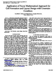
where L value (0 ≤ L ≤ 1) represents the overall DM satisfaction under the proposed strategy of minimizing the most possible value. If L = 1 then each goal is fully satisfied; If 0 < L < 1 then all of the goals are satisfied at the level L; if L = 0, then none of the goals are satisfied. The PLP approach provides the overall degree of DM satisfaction. Step 7 The model is solved and modified interactively. If the DM is not satisfied with the initial solution, then the model must be modified until a satisfactory solution is found. NUMERICAL EXAMPLE Here, we present a numerical example to illustrate the model. The application of the model is performed for a hypothetical data and the considered supply chain network includes two suppliers, which are located in
different countries in Europe, a manufacturer, four subcontracts, two retailers and four customers in different cities in Turkey. The supply chain network that is structured to transport textile industry products from suppliers to customers is constituted from multicomponents, multi-echelon by APP (Figure 2). In the numerical example, manufacturer receives components (Figure 3) from suppliers to serve the retailers. But because of the production costs and different demands, company works with four subcontracts to answer customers. Manufacturer decides APP with six term planning horizon in supply chain capacity board. If amount receiving from suppliers and subcontracts are more than demand of retailers, it becomes inventory also its reverse, company faces backorder costs. Solution The solution procedure of the proposed APP problem under Fuzzy material requirement constraints is demonstrated as follows: First, the original APP model is formulated under Fuzzy material requirement according to the Equations 1 to 27. Secondly, all the Fuzzy inequality constraints are converted to crisp ones using weighted average method at α = 0.5 . The original problem is solved using the ordinary single-objective LP problem to obtain the initial solutions for each of the objective functions, with the assumption that the DM specified the most likely value of the triangular distribution of each Fuzzy number as the precise value. The model is solved by using LINGO solver on a Pentium IV 3.2 GHz personal computer with 3 seconds CPU time
3394
Sci. Res. Essays
End item
Figure 3. The bill of material.
Table 9. Initial solutions and interval values for each of the Fuzzy objective functions.
Item Obj.function L Z1 Z2 Z3
LP-1 Min Z1
LP-2 Max Z2
41402.7
7195.35
LP-3 Min Z3 -
(zi
5413.33
PIS
NIS
; zi ) 41402.7; 71953.5 7195.35; 4140.27 5413.33; 9084.89
Initial solutions Max L 0.1892 44978 4498 5754
Table 10. Improved solutions and interval values for each of the Fuzzy objective functions.
Item Obj.function L Z1 Z2 Z3
LP-1 Min Z1
LP-2 Max Z2
41402.7
19325.4
LP-3 Min Z3 -
13662.2
for the parameters presented in Tables 1 to 8 with the intention of obtaining optimal values. The resulting ordinary single-objective LP model for solving the APP problem can be formulated according to Equation (38). This LP problem is solved by using LINGO. Using the model, the objective values of the initial solutions are Min Z1 = $41402.7, Max Z2 = $7195.35 and Min Z2 = $5413.33 (Table 9). Additionally, we attempt to modify the PIS and NIS for each of the Fuzzy objective functions to yield a satisfactory solution. Consequently, the improved solutions are Z1 = $52291.45, Z2 = $13062.83, Z3 = $16433.43 (Table 10). Table 10 lists the optimal plan for the Example. In the Tables 9, 10 and 12, the initial values for the PIS and NIS of the Fuzzy objectives can be specified as NIS PIS NIS PIS (Z1 , Z1 ) = (41402.7; 71953.5), (Z2 , Z2 ) = NIS PIS (7195.35; 4140.27) and (Z3 , Z3 ) = (5413.33; 9084.89). The resulting objective values of the initial solutions are Z1 = $44978, Z2 = $4498, Z3 = $5754. We attempt to
(zi
PIS
NIS
; zi ) 41402.7; 71953.5 19325.4; 10481.1 13662.2; 25106.2
Improved solutions Max L 0.5649 52291.45 13062.83 16433.43
improve the initial solutions and then PIS and NIS values NIS PIS of Fuzzy objectives are updated as (Z1 , Z1 ) = NIS PIS (41402.7; 71953.5), (Z2 , Z2 ) = (19325.4; 10481.1) NIS PIS and (Z3 , Z3 ) = (13662.2; 25106.2). Consequently, the improved solutions are Z1 = $52291.45, Z2 = $13062.83, Z3 = $16433.43. Applications of this kind of production/distribution models to the real cases are really hard. Because these models defined NP-hard problems and when the size of the model is enlarged, obtaining the optimal solutions will be nearly impossible in normal conditions. In this area, more proposed models validated by numerical examples are presented in which the case studies are applied to real supply chains (Mula et al., 2010). Conclusion In this study, a supply chain network design problem is modeled with consideration of a supply chain functions in
Paksoy et al.
3395
Table 11. Optimal distribution plan for the example.
Obj. function
L=0.5649; Z1=52291.45; Z2=13062.83; Z3=16433.43; ~ z = ( 39228.62 , 52291.45, 68724.88 )
Period
1 A111=232.6 A121=286.92 A211=329 A221=274.68
2 A112=250.60 A122=7 A212=141.39 A222=385
3 A113=385 A123=399 A213=175 A223=161
B12=1.5 B22=82.5
B23=120
D1211=99.68 D1221=122.96 D1311=40.11 D1321=40.11 D2211=141 D2221=117.72
D1122=3 D1212=107.40 D2112=3 D2212=57.59 D2222=165
D1213=165 D1223=171 D2123=0 D2213=75 D2223=69
Ekp
E11=80 E21=200
E12=80 E22=200
E13=200 E23=200
Fklp
F121=10 F141=70 F221=60 F211=70 F231=70
F132=10 F142=70 F212=70 F222=70 F232=60
P1=216 O1=64.8 W1=108 H1=18
P2=196
Aitp
Bjp
Dijtp
Pp Op Wp Hp Fp Wp Ip Bp
B21=120.34 B31=20.05
W2=108
4 A114=385 A124=385 A214=148.33 A224=148.33 B14=111.57 B24=2.71 B44=19.04 D1114=159.57 D1124=165 D1214=5.42 D2114=63.57 D2124=58.15 D2224=5.42 D2414=38.09 D2424=38.09
F113=190 F143=10 F223=70 F233=70 F243=60
P3=216 O3=64 W3=108
5 A125=77 A215=392 A225=315
B15=67.5 B25=16.5
B16=85.5
D1116=165 D2116=6 D2126=171
E14=200 E24=200
E15=80 E25=200
E16=200 E26=85
F124=60 F134=70 F144=70 F214=190 F224=10
F125=10 F145=70 F215=70 F225=60 F235=70
F116=55 F126=70 F146=75 F216=15 F236=70
P4=216 O4=50.66 W4=108
P5=196
P6=199.5
W5=99.75
W6=99.75
F5=8.25
Table 12. The (PIS; NIS) values for each of the Z1, Z2 and Z3.
Initial solutions 41402.7; 71953.5 7195.35; 4140.27 5413.33; 9084.89 44978 4498 5754 0.1892
A116=385 A216=14 A226=399
D1225=33 D2115=135 D2125=135 D2215=33
W0=90 I0=40 B0=181.2
Item NIS PIS (Z1 , Z1 ) NIS PIS (Z2 , Z2 ) NIS PIS (Z3 , Z3 ) Z1 Z2 Z3 L
6
Improved solutions 41402.7;71953.5 (19325.4; 10481.1 (13662.2; 25106.2 52291.45 13062.83 16433.43 0.5649
3396
Sci. Res. Essays
which customer demand and capacities in production environment are Fuzzy. A linear programming is adapted to this model to solve the problem. Model is set with different kinds of functions such as multi components, multi periods, APP and material requirement constraints etc. Minimizing the total transportation, regular, overtime and subcontracts production and human resources costs under these constraints is aimed in the model. The plan obtained in this way implies supply chain management of the trade-off between the minimization of the costs and fill rate of market demand and also along with APP. The linear programming model is solved by LINDO package program and the results are discussed. In this paper, we constituted a small sized model with constraints as mentioned. Computational experiments were conducted with the proposed model for the case of a general appliance company for evaluation of the benefits of the integrated production–distribution planning in supply chain management model proposed here as compared to the crisp and disinter-grated approaches. The illustrated model consists of five echelons which include actors order by suppliers, subcontracts, manufacturer, retailers and customers. Proposed model provides that DMs can determine both minor constraints (regular, overtime, subcontract production and human resources such as APP) and major constraints (whole supply chain capacities and transportation costs) together. We try to develop a linear programming model to make APP in supply chain systems under Fuzzy material requirement constraints. The proposed model yields a compromise solution and the DMs overall levels of satisfaction, given these solved Fuzzy values. Moreover, the proposed model provides a systematic framework that facilitates the decision-making process, enabling a DM interactively to modify the membership functions of the parameters until a satisfactory solution is obtained. Consequently, the proposed model is the most practically applicable for making APP decisions. The model can be expanded by considering alternative transportation modes between echelons for each point pairs. In that situation new decision variables emerges and the model complexity increases. It is obvious that managing the supply chain network design problem is a comprehensive topic and there are additional variables and parameters which can be embedded to the model. For example, a vehicle routing problem to determine the number of carriers or their capacities that will realize the transportation between echelons and multi products can also be added to the model. This type of large sized models is NP-complete. However, approximate results can easily be obtained for complex problems by using various simulation techniques or heuristics, such as, simulated annealing, genetic algorithms etc. The research is continued in direction of further extension of the proposed production–distribution aggregate planning model by representing additional sources of uncertainty such as Fuzzy lead times, Fuzzy supplier reliability etc.
NOMENCLATURE Total Suppliers Number: 2 Total Retailers Number: 2 Total Periods Number: 6 Total Manufacturer Number: 1 Total Subcontracts Number: 4 I0: 40, B0: 0, W0: 90, k: 4, :8 Total Customers Number: 4 Total Components Number: 2 Wpmax :110, Ipmax :100 Bpmax :100; 1,2,3,4,5,6: %50 1,2,3,4,5,6:%30; 1,2,3,4,5,6:%20 1,2,3,4,5,6: %10; %30 REFERENCES Ahumada O, Villalobos JR (2009). Application of Planning Models in the Agri-Food Supply Chain: A Review. Eur. J. Oper. Res., 196 (1): 1-20. Aliev RA, Fazlollahi B, Guirimov BG (2007). Fuzzy-Genetic Approach to Aggregate Production–Distribution Planning in Supply Chain Management. Inf. Sci., 177 (20): 4241-4255. Cohen MA, Lee HL (1989). Resource Deployment Analysis of Global Manufacturing and Distribution Networks. J. Manufact. Oper. Manage., 2: 81-104. Elion S (1975). Five Approaches to Aggregate Production Planning. AIIE Trans., 7: 118-131. Foo CYD, Mike BL, Raymond R, Jenny S (2008). A Heuristic-Based Algebraic Targeting Technique for Aggregate Planning in Supply Chains. Comput. Chem. Eng., 32 (10): 2217-2232. Gen M, Syarif A (2005). Hybrid Genetic Algorithm for Multi-Time Period Production Distribution Planning. Comput. Ind. Eng., 48: 799-809. Goodman DA (1974). A Goal Programming Approach to Aggregate Planning of Production and Work Force. Manage. Sci., 20: 15691575. Gunasekaran A, Ngai E (2009). Modeling and Analysis of Build-ToOrder Supply Chains. Eur. J. Oper. Res., 195(2): 319-334. Hanssmann F, Hess SW (1960). A Linear Programming Approach to Production and Employment Scheduling. Manage. Sci., 1: 46-51. Jamalnia A, Soukhakian MA (2009). A Hybrid Fuzzy Goal Programming Approach with Different Goal Priorities to Aggregate Production Planning. Comput. Ind. Eng., 56 (4): 1474-1486. Lai YJ, Hwang CL (1992). A New Approach to Some Possibilistic Linear Programming Problems. Fuzzy Sets and Systems, 49(2): 121-133. Leung CH, Chan SW (2009). A Goal Programming Model for Aggregate Production Planning with Resource Utilization Constraint. Comput. Ind. Eng., 56 (3): 1053-1064. Liang T (2008). Fuzzy Multi-Objective Production/Distribution Planning Decisions with Multi-Product and Multi-Time Period in a Supply Chain. Comput. Ind. Eng., 55: 676-694. Liang T, Cheng HW (2009). Application of Fuzzy Sets to Manufacturing/Distribution Planning Decisions with Multi-Product and Multi-Time Period in Supply Chains. Expert Systems with Applications, 36: 3367-3377. Masud ASM, Hwang CL (1980). Aggregate Production Planning Model and Application of Three Multiple Objectives Decision Methods. Int. J. Prod. Res., 18: 741-752. Mula J, Peidro D, Diaz-Madronero M, Vicens E (2010). Mathematical Programming Models for Supply Chain Production and Transport Planning. Eur. J. Oper. Res., 204: 377-390. Paksoy T (2005). Distribution Network Design and Optimization in Supply Chain Management: A Strategic Production-Distribution Model under Material Requirements Constraints. J. Selcuk Univ. Soc. Sci. Inst. Turk., 14: 435-454. Paksoy T, Atak M (2005). A Stochastic Approach to Interactive Fuzzy Multi-Objective Linear Programming for Aggregate Production Planning. Selçuk J. Appl. Math., 6 (2): 79-98.
Paksoy et al.
Paksoy T, Güles HK, Bayraktar D (2007). Design and Optimization of a Strategic Production-Distribution Model For Supply Chain Management: Case Study of a Plastic Profile Manufacturer in Turkey. Selçuk J. Appl. Math., 8: 883-99. Pyke DF, Cohen MA (1993). Performance Characteristics of Stochastic Integrated Production-Distribution Systems. Eur. J. Oper. Res., 68 (1): 23-48. Sarker BR, Diponegoro A (2009). Optimal Production Plans and Shipment Schedules in a Supply-Chain System with Multiple Suppliers and Multiple Buyers. Eur. J. Oper. Res., 194 (3): 753-773. Schütz P, Tomasgard A, Ahmed S (2009). Supply Chain Design under Uncertainty Using Sample Average Approximation and Dual Decomposition. Eur. J. Oper. Res., 199(2): 409-419. Sourirajan K, Ozsen L, Uzsoy R (2009). A Genetic Algorithm for a Single Product Network Design Model with Lead Time and Safety Stock Considerations. Eur. J. Oper. Res., 197 (2): 599-608. Syarif A, Yun Y, Gen M (2002). Study on Multi-Stage Logistics Chain Network: A Spanning Tree-Based Genetic Algorithm Approach. Comput. Ind. Eng., 43 (1): 299-314. Tingley GA (1987). Can ms/or sell itself well enough? Interfaces, 17: 4152. Tuzkaya U, Önüt S (2009). A Holonic Approach Based Integration Methodology for Transportation and Warehousing Functions of the Supply Network. Comput. Ind. Eng., 56: 708-723. Wang HS (2009). A Two-Phase Ant Colony Algorithm for Multi Echelon Defective Supply Chain Network Design. Eur. J. Oper. Res., 192(1): 243-252.
3397
Wang RC, Fang HH (2001). Aggregate Production Planning with Multiple Objectives in a Fuzzy Environment. Eur. J. Oper. Res., 133: 521-536. Wang RC, Liang T (2004). Application of Fuzzy Multi-Objective Linear Programming to Aggregate Production Planning. Comput. Ind. Eng., 46(1): 17-41. Wang RC, Liang T (2005). Applying Possibilistic Linear Programming to Aggregate Production Planning. Int. J. Prod. Econ., 98(3): 328-341. Williams JF (1981). Heuristic Techniques for Simultaneous Scheduling of Production and Distribution in Multi-Echelon Structures: Theory and Empirical Comparisons. Manage. Sci., 27 (3): 336-352. Yan H, Yu Z, Cheng TCE (2003). A Strategic Model for Supply Chain Design with Logical Constraints: Formulation and Solution. Comput. Oper. Res., 30(14): 2135-2155. Yılmaz P (2004). Strategic Level Three-Stage Production Distribution Planning with Capacity Expansion. Unpublished Master Thesis. Sabanci University Graduate School of Engineering and Natural Sciences, in Turkish, pp. 1-20. You F, Grossmann E (2008). Design of Responsive Supply Chain under Demand Uncertainty. Comput. Chem. Eng., 32(12): 3090-3111.