ARCHIVES OF ACOUSTICS 34, 4, 491–505 (2009)
Application of Hilbert Transform-Based Methodology to Computer Modelling of Reverberant Sound Decay in Irregularly Shaped Rooms Mirosław MEISSNER Institute of Fundamental Technological Research Polish Academy of Sciences Pawińskiego 5B, 02-106 Warszawa, Poland e-mail:
[email protected] (received June 30, 2009; accepted September 21, 2009 ) A study into the application of the Hilbert transform in numerical simulations of reverberant sound decay in irregularly shaped enclosures is presented. It is shown that there are some limitations in the use of this integral transform to exponentially decaying harmonic signals because the integration result consists not only of a signal, which differs from the original one by a phase shift of π/2, but also of a decaying nonoscillating signal occurring due to the fact that a spectrum of exponential function is unbounded. An initial amplitude of this signal is directly proportional to the ratio between a damping coefficient and a mode frequency, thus for lightly damped rooms, where this ratio is much smaller than unity, it can be neglected. Results of numerical simulation carried out for L-shaped enclosure indicate that the Hilbert transform is a useful tool in calculating instantaneous properties of reverberant sound, especially an envelope of the sound pressure level. It is of special importance in the case of irregularly shaped rooms, where a deviation from the exponential sound decay often occurs because of differences between reverberant responses for particular modes. Keywords: Hilbert transform, analytic signal, irregularly shaped enclosures, reverberant room response, reverberation time, early and late decay times.
1. Introduction Over the last few decades, the Hilbert transform found several practical applications for the analysis and identification of vibration signals in a time domain [1, 2]. An appropriate use of the Hilbert transform to a vibration signal provides some additional information about amplitude, instantaneous phase and vibration frequency. This information is valid when employed to the study of non-linear vibrations [3]. The Hilbert transform-based techniques are a convenient tool to use in dealing with bandlimited signals and in this situation, they
492
M. Meissner
offer new methods for a damage diagnosis [4, 5] and time-varying vibration decomposition [6, 7]. In room acoustics, a utility of Hilbert transform is manifested in low-frequency range, where acoustic modes are well separated, and in this case it is used to obtain a smooth decay curve for noisy single and multi-mode reverberant room responses [8]. In a numerical modelling of temporal sound decay in enclosures, an application of Hilbert transform is a simple way to get information about an envelope and the phase of a decaying acoustic signal. It is especially important in a simulation of reverberant response of coupled spaces or rooms having irregular shape because differences between modal responses, observed in these cases, can lead to nonlinear profiles of pressure level decay [9] or double slope sound decay [10, 11]. In the first part of this paper, the most important properties of Hilbert transform are shortly discussed. Then, the study is focused on an application of the transform to exponentially decaying cosine and sine functions that model the reverberation behaviour of a single mode. It is revealed that a use of the Hilbert transform is limited to decaying signals for which the ratio between a damping coefficient and a mode frequency is much smaller than unity. In the last part, a utility of Hilbert transform is demonstrated using sound decay simulations performed for the enclosure having a shape resembling the capital letter L. 2. Theoretical background The Hilbert transform plays an important role in a signal analysis because it can be used in a direct examination of instantaneous properties of the signal such as: an amplitude, a phase and a frequency. The Hilbert transform H of a real function f (t) is defined as Z∞ Z∞ 1 f (t) 1 f (t − τ ) ˆ H[f (t)] = f (t) = dτ = dτ, (1) π t−τ π τ −∞
−∞
where the integral is considered as a Cauchy principal value because of the possible singularity at τ = t or τ = 0. As it results from Eq. (1), the Hilbert transform represents a convolution between the transformer 1/πt and the function f (t), which may be written as fˆ(t) = (1/πt) ∗ f (t). The double use of the Hilbert transform yields the function f (t) with an opposite sign, hence it carries out the phase shift of π from the initial signal. Thus, the Hilbert transform is often interpreted as the π/2 phase shift operator. The signal f (t) and its Hilbert transform fˆ(t) are related to each other in such a way that they together create the so-called analytic signal a(t) defined as a(t) = f (t) + j fˆ(t) = E(t)ej ψ(t) , (2) q where E(t) = f 2 (t) + fˆ2 (t) is the amplitude (envelope, magnitude) of the analytic signal and ψ(t) = tan−1 [fˆ(t)/f (t)] is the phase of a(t). The instantaneous
Application of Hilbert Transform-Based Methodology. . .
493
angular frequency of a(t) is defined as: ω(t) = dψu / dt, where ψu (t) is the continuous, unwrapped phase, i.e. ψu (t) = ψ(t) + Γ (t),
(3)
where Γ (t) is an integer multiple of π-valued function designed to ensure a continuous phase function. Accurately computed, the derivatives of the discontinuities in Γ (t) and ψ(t) cancel. Note that if the Γ (t) is omitted, there will be δ functions at various t in ω(t). The analytic representation of real signals has been found very useful for many types of signals, especially for the amplitude-modulated ones, modeled as a product of the bandlimited signal g(t) and the high-pass oscillating signal u(t). If the Fourier transform of g(t) satisfies the condition F[g(t)] = 0 for |ω| ≥ ωc , where ωc is the so-called cutoff frequency, and u(t) is a signal with the Fourier transform equal to zero for |ω| < ωc , then [12] H[g(t)u(t)] = g(t)H[u(t)],
(4)
thus, to compute the Hilbert transform of the product of a low-pass signal with a high-pass signal, only the high-pass signal needs to be transformed. 3. Hilbert transform in room acoustics In room acoustics the Hilbert transform is found to be a useful tool in a signal analysis in a frequency range bounded from above by the so-called “Schroeder frequency” given by [13] p ωs = 2πc 6/A, (5) where c is the sound speed and A is the total room absorption. Below this frequency the mode density is low and particular modes can be decomposed from a room response to an acoustic excitation, thus in multi-mode resonance systems the "Schroeder frequency" marks the transition from individual, well-separated resonances to many overlapping modes. Consequently, in low-frequency range, the room behaves like a resonance system, with specific acoustic modes, whose characteristics such as: an amplitude distribution, a mode frequency and a damping factor, depend on the room shape and absorption properties of room walls. If a sound source located inside the room operates with constant power, energy losses on the absorbing walls are covered by the source and in the steady-state, which is usually reached during short time after a source start, the absorptive power is equal to that produced by the source. When the sound source is switched off, the acoustic energy accumulated inside the room is dissipated on walls and a reverberation due to the common decaying of modes occurs. In the case of a single mode, a temporal decay of a sound pressure can be described simply by the exponentially decaying harmonic function [14] pm (t) = Am e−rm t cos(Ωm t − βm ),
(6)
494
M. Meissner
where t ≥ 0 is the time, m = 1, 2, 3... is the mode number, Am is the initial mode amplitude, rm > 0 is the damping coefficient, Ωm is the mode frequency for oscillations with a damping p 2 − r2 , Ωm = ωm (7) m where ωm is the mode frequency, βm is the initial phase of modal response · ¸ 2 2 −1 rm (ωm + ω ) βm = tan , (8) 2 − ω2) Ωm (ωm where ω is the sound source frequency. Unfortunately, in the analysed case the property (4) of Hilbert transform can not be applied, because the exponentially decaying signal e−rm t has the Fourier transform [5] 1 F(e−rm t ) = √ , (9) 2π(rm + j ω) thus, its spectrum is unbounded. As follows from Eq. (6), the finding of H[pm (t)] requires a computation of the Hilbert transform of two harmonic functions: cm (t) = e−rm t cos(Ωm t) and sm (t) = e−rm t sin(Ωm t). Applying the second expression for the Hilbert transform from Eq. (1) to the first function, we obtain the integral Z∞ −rm |t−τ | 1 e cos[Ωm (t − τ )] cˆm (t) = dτ, (10) π τ −∞
where an absolute value in the exponent assures the boundedness of the exponential function. In a method for evaluation of the integral in Eq. (10), we use the following substitution Z∞ 1 = e−qτ dq, (11) τ 0
and the final result, after some transformations, is given by cˆm (t) = e−rm t sin(Ωm t) + f1 (t), 2γm f1 (t) = π
Z∞ 0
(1 − s2 )e−ωm st ds , (s2 + 2γm s + 1)(s2 − 2γm s + 1)
(12) (13)
where γm = rm /ωm . An application of a similar integration method to the second harmonic function yields sˆm (t) = −e−rm t cos(Ωm t) + f2 (t), f2 (t) =
4γm
p
2 1 − γm π
Z∞ 0
se−ωm st ds . (s2 + 2γm s + 1)(s2 − 2γm s + 1)
(14) (15)
Application of Hilbert Transform-Based Methodology. . .
495
Since a use of the Hilbert transform to the cosine and sine functions gives H[cos(Ωm t)] = sin(Ωm t),
(16)
H[sin(Ωm t)] = − cos(Ωm t), the functions f1 and f2 on right-hand sides of Eqs. (12) and (14) may be interpreted as corrections of Eq. (4) due to the fact that a spectrum of exponentially decaying signal is unbounded. For the parameter γm equal to zero, the correction functions f1 and f2 vanish and Eqs. (12) and (14) reduce to Eqs. (16). In order to investigate behaviours of f1 and f2 for non-zero values of γm , it is necessary to determine first the limit values of rm and ωm . In a low-frequency range, typical materials covering room walls are characterized by low sound absorption, thus the case studied is a hard-walled, lightly damped room with a reverberation time of the order of one second at mid and high frequencies, but much longer decay times at low modal frequencies. The modal reverberation time Tm , defined as that for which the pressure level decays by 60 dB in a mode, is related to the damping coefficient by the expression [16] Tm =
3 ln(10) , rm
(17)
thus, it is inversely proportional to rm . Now, if we assume that a low limit of Tm is of the order of two seconds, we easily find: (rm )max ' 3.45 s−1 . Since a minimum value of ωm corresponds to the lowest audible frequency, the parameter γm has the upper limit (γm )max ' 0.028. In the case of a decay of single acoustic mode, the reverberation time Tm determines a time limit above which temporal variations in the sound pressure have a very small influence on perceived sound. Thus, an analysis of temporal behaviour of the functions f1 and f2 may be limited to the time interval from zero to Tm . To evaluate contributions of f1 and f2 in cˆm and sˆm , respectively, we consider the relative correction functions: fr1 = f1 /e−rm t and fr2 = f2 /e−rm t . Figure 1 shows dependences of these functions on the non-dimensional time parameter t/Tm for different values of γm . The graphs in Fig. 1a indicate that the function f1 contributes to cˆm significantly, especially for t/Tm close to unity, and in the range of t/Tm from 0.1 to 1, values of the relative function fr1 drop four times with a double decrease in the parameter γm . In the case of the function fr2 a situation is much more favourable, because for (γm )max its values for t/Tm from the interval 0.05–1 do not exceed 0.001 and for t/Tm from the range 0.1–1, values of fr2 fall down eight times with a double decrease in γm (Fig. 1b). The function fr2 appears visibly larger for the smallest values p of t/Tm 2 /π, and for t/Tm equal to zero it has the maximum value given by 2γm 1 − γm because
496
M. Meissner
Fig. 1. Changes in relative correction functions fr1 and fr2 with non-dimensional time parameter t/Tm for different values of γm .
Z∞ 0
s ds ' 2 (s + 2γm s + 1)(s2 − 2γm s + 1)
Z∞ 0
1 s ds = 2 + 1) 2
(s2
(18)
for the parameter γm much smaller than unity. In real conditions, when there are multiple modes in the room system, a reverberant room response for non-overlapping modes is of the form [14] M √ X p(r, t) = V Am e−rm t cos(Ωm t − βm )Φm (r),
(19)
m=1
where Φm (r) are orthogonal eigenfunctions normalized in the room volume V , r = (x, y, z) is the position vector and the mode M is the last mode whose frequency is smaller than the “Schroeder frequency” ωs . In Eq. (19) the Helmholtz mode A0 e−r0 t representing a trivial solution of the wave equation was omitted because it is not perceived as a sound. For lightly damped rooms the modal amplitude Am hardly depends on the sound source frequency [14]. Moreover, the absolute value of Am reaches a maximum when the frequency ωm is very close to ω. A reverberant room response to a harmonic excitation is then dominated by modes with frequencies lying in the nearest vicinity of ω. As it results from Eq. (8), when the condition ωm ' ω is satisfied, the phase βm is equal to π/2, approximately, thus for the dominant mode a temporal decay of sound pressure is pm (t) ' Am e−rm t sin(Ωm t).
(20)
Using Eq. (14) it is easily found that the amplitude and the phase of this function are q E1 = Am e−2rm t − f2 (t)e−rm t cos(Ωm t) + f22 (t), (21) £ ¤ −1 rm t ψ1 = tan − cot(Ωm t) + f2 (t)e / sin(Ωm t) .
Application of Hilbert Transform-Based Methodology. . .
497
Figure 2 depicts changes in ∆Er = |(E1 − E)/E| and ∆ψr = |(ψ1 − ψ)/ψ| with the non-dimensional time parameter t/Tm , where E = Am e−rm t and ψ = Ωm t − π/2. Thus, the quantities ∆Er and ∆ψr may be interpreted as relative errors in predictions of amplitude and phase for decaying dominant modes, when the Hilbert transform-based methodology is used. The data presented in Fig. 2 was obtained for the most unfavourable case when the parameter γm is maximal. Due to the occurrence of cosine and sine functions in expressions for E1 and ψ1 , the parameters ∆Er and ∆ψr are oscillatory in character and the frequency of oscillation corresponds to the mode frequency ωm .
Fig. 2. Relative errors ∆Er and ∆ψr in predictions of amplitude and phase for dominant modes versus non-dimensional time parameter t/Tm for maximum value of γm . Calculation parameters: rm = 4 s−1 , ωm = 142.9 rad/s.
The graphs in Fig. 2 show that the relative errors ∆Er and ∆ψr are visibly smaller than unity in a range of t/Tm from 0 to 0.01 and they appear to be sufficiently small for the remaining values of t/Tm . From a viewpoint of room acoustics, this is a very important property because it enables us to avoid significant errors in prediction of the reverberation time or decay times in a late stage of sound decay. Note, that the upper envelope of the function describing changes in ∆Er with t/Tm has a shape of function fr2 for the maximum value of γm (Fig. 1b). Another kind of modes are the so-called non-dominant modes. For the considered case of lightly damped enclosures, they have slight influence on reverberant room response. Non-dominant modes can be defined as these for which the sound source frequency ω is considerably smaller or considerably larger than the mode frequency ωm . In such a case, the expression (8) for the phase βm can be simplified to the form p 2 ), βm = ± tan−1 (γm / 1 − γm (22) where the plus and minus signs correspond to the cases: ω ¿ ωm and ω À ωm , respectively. Since the parameter γm is assumed to be much smaller than unity,
498
M. Meissner
a temporal decay of sound pressure for non-dominant modes can be approximately determined by pm (t) ' Am e−rm t cos(Ωm t). (23) Applying Eq. (12), relative errors in predictions of amplitude and phase were found. Calculation results shown in Fig. 3 prove that for non-dominant modes the errors ∆Er and ∆ψr are visibly larger as compared to the dominant modes. Moreover, similarly as before, the upper envelope of the function describing variations in ∆Er with t/Tm corresponds to the function fr1 determined for the maximum value of γm (Fig. 1a).
Fig. 3. Relative errors ∆Er and ∆ψr in predictions of amplitude and phase for non-dominant modes versus non-dimensional time parameter t/Tm for maximum value of γm . Calculation parameters: rm = 4 s−1 , ωm = 142.9 rad/s.
4. Numerical simulation A primary objective of a numerical simulation was to demonstrate the utility of the Hilbert transform technique in computational predictions of a reverberant sound decay in rooms of complex geometry. In the present study, an enclosure having shape resembling the capital letter L is considered (Fig. 4). For this room geometry, a computation of eigenfunctions was possible only through numerical methods. It was found [17] that for lightly damped rooms, a distribution of modes amplitude is well approximated by eigenfunctions computed for perfectly rigid room walls. Thus, using double indexed quantities we can write √ Ψn (x, y)/ h, m = 0, n > 0, Φmn (r) = p (24) 2/h cos(mπz/h)Ψ (x, y), m > 0, n > 0, n where h is the room height and the eigenfunctions Ψn are normalized over a horizontal section of the room. In this case, the modal frequencies are given by r³ mπc ´2 ωmn = + ωn2 , (25) h
Application of Hilbert Transform-Based Methodology. . .
499
where ωn is an eigenfrequency for the function Ψn . The functions Ψn and the frequencies ωn were computed with the aid of numerical technique based on the forced oscillator method [18] with finite difference algorithm. Determination of the eigenfunctions Φmn makes possible a calculation of modal amplitudes and damping coefficients [14] R ωmn c2 Q(r)Φmn (r) dv r h V (26) Amn = i, 2 2 2 2 2 Ωmn V (ωmn − ω ) + 4rmn ωmn ρc2 rmn =
R S
Φ2mn (r) ds
, (27) 2Z where Q(r) is the volume source distribution and Z is the wall impedance.
Fig. 4. Analysed room having the shape resembling a capital letter L.
In the numerical simulation it was assumed that dimensions of a room are the following (in meters): d1 = d2 = 3, l1 = 4, l2 = 6, h = 3 and the sound source with the power of 0.1 W was modelled by a point source at the location (in meters): x = 4, y = 4, z = 1. It was also postulated that an absorbing material with the random-absorption coefficient α of 0.07 was uniformly located on room walls. The wall impedance Z was assumed to be a real number, i.e., the mass and stiffness of the absorbing material are neglected. A value of Z was found from the well-known relationship between the coefficient α and the impedance ratio ξ [19] · ¸ 8 1 2 α= 1+ − ln(1 + ξ) , ξ = Z/ρc. (28) ξ 1+ξ ξ Since the total room absorption A for an uniform distribution of absorbing material on room walls is determined by: A = αS, the “Schroeder frequency” calculated from Eq. (5) assumes the value fs = ωs /2π ' 230 Hz. In a frequency
500
M. Meissner
range bounded from above by the “Schroeder frequency”, 212 eigenmodes were found. For this set of modes, a reverberant sound decay in an observation point located at the position (in meters): x = 8, y = 2, z = 1.8, was simulated and the Hilbert transform-based technique was used to calculate an envelope of this decay. Allowing for theoretical considerations in Sec. 3, in calculations of the Hilbert transform the correction function f1 and f2 were omitted. Results of a numerical simulation presented in Fig. 5 show for two source frequencies a decay of sound pressure in the time interval corresponding approximately to the reverberation time (Fig. 5b,d) and illustrate additionally an evolution of sound pressure in the early stage of sound decay (Fig. 5a,c). In the initial stage of decay, the acoustic signal together with its upper and lower envelopes computed via the Hilbert transform are depicted. The data in Fig. 5b,d indicate that an excitation of room by a tone of 93 Hz results in almost a smooth decrease in the sound pressure, whereas a source signal with a frequency of 96 Hz gives a sound decay with a characteristic wavy envelope. Such a difference between forms of a sound decay is associated with a great influence of the source
Fig. 5. Temporal decay of sound pressure p for two frequencies of sound source: (a,b) 93 Hz and (c,d) 96 Hz.
Application of Hilbert Transform-Based Methodology. . .
501
frequency on the modal amplitude Amn . As it is evident from Fig. 6, for the frequency of 93 Hz there is one strong dominant mode because the mode frequency fmn corresponds almost exactly to the source frequency. When the source frequency is shifted to 96 Hz there are two significant modes of slightly different frequencies. In this case an envelope of a sound pressure begins to fluctuate with a frequency equal to the difference between frequencies of these neighbouring modes (beating effect).
Fig. 6. Absolute value of modal amplitude Amn versus mode frequency fmn for sound source frequencies: a) 93 Hz and b) 96 Hz.
An important thing in investigations of reverberant phenomenon is a decay time estimation which is based in practice on fitting a straight line to the decay envelope of pressure level L = 20 log(|p|/p0 ). The reference pressure p0 is selected in such a way that for t = 0 the level L is equal to zero. The linear fitting is realized by the least-squares method (linear regression) and it gives good results when decay times of dominant modes are very similar. If it is not satisfied, a difference between the early decay time (EDT) and the late decay time (LDT) may occur, where LDT is the 60 dB decay time calculated by a line fit to the portion of a decay curve between −50 and −60 dB [10]. Calculation results presented in Fig. 7a show that the envelope LE of pressure level found for the source frequency of 93 Hz appears to be smooth enough and a fitting line matches the envelope reasonably well. It is obviously a consequence of a strong dominance of one acoustic mode in a reverberant room response. In this case the estimation of a reverberation time from a slope of the fitting line gives a result T60 ' 2.27 s. For the second source frequency, the envelope LE is deformed by fluctuations due to the beating effect, but the mean trend in a decrease of the pressure level is well reproduced by the straight line (Fig. 7b). A reverberation time calculated from a slope of fitting line is T60 ' 2.24 s, thus it is almost the same result as in the case of the first source frequency.
502
M. Meissner
Fig. 7. Envelope LE of the pressure level for source frequencies: a) 93 Hz and b) 96 Hz. Straight lines correspond to best-fit lines determined by regression method.
In the last numerical example, a reverberant sound decay in the observation point for the source frequency of 144 Hz will be examined. Simulation data depicted in Fig. 8 present temporal changes in the sound pressure p and the interesting thing to note is that a sound pressure appears to grow, instead of decrease, in the initial stage of reverberation process. This behaviour of sound pressure results in untypical temporal changes in the pressure level because its envelope LE exhibits “ballooned” appearance with a slow initial decay and a visibly faster late decay (Fig. 9a). The opposite of this manner of sound decay is a reverberation process with a rapid early decay and a shallow late decay. In such a situation a decay curve possesses the so-called “sagging” appearance which occurs more frequently in practice [20].
Fig. 8. Temporal decay of sound pressure p for source frequency of 144 Hz.
In Fig. 9a a smooth curve described by the function F (t) represents a best-fit curve determined by a polynomial regression. A “ballooned” shape of pressure
Application of Hilbert Transform-Based Methodology. . .
503
Fig. 9. (a) Envelope LE of pressure level for source frequency of 144 Hz. Function F (t) corresponds to best-fit curve calculated by polynomial regression. (b) Reverberation time T60 estimated from slope of fitting curve.
level decay can be quantified by estimating the early and late decay times from a slope of the best-fit curve. Applying a classical linear fitting to appropriate portions of this curve we obtain: EDT = 4.02 s and LDT = 2.05 s. Because of high nonlinearity of the function F (t) in the early stage of sound decay, an estimation of EDT from a temporal dependence of the reverberation time T60 seems to be more accurate. This time is determined from a slope of the best-fit curve, i.e. 60 T60 = − (29) dF (t)/dt and changes in T60 with the time t are shown in Fig. 9b. In this approach EDT is thought as the mean value of T60 in a time interval corresponding to a decrease in F (t) from 0 to −10 dB. The early decay time computed by this method is 4.64 s, thus it differs visibly from the value of EDT estimated by a linear regression. A use of this calculation technique to an estimation of late decay time gives the same result as in the case of linear fitting. 5. Conclusions In room acoustics, the usefulness of Hilbert transform is evinced in a frequency range bounded from above by the “Schroeder frequency”, which represents a limit between well separated room modes below it and many overlapping modes above it. When a sound decay in reverberant enclosures is studied, an application of Hilbert transform is a simple way to get information about the envelope and phase of a decaying acoustic signal. This is of great significance in the case of irregularly shaped rooms where deviations from the exponential sound decay, leading to non-linear profile of decay curve, often occur because of differences between reverberant responses for particular modes.
504
M. Meissner
The important result of this study is finding that there are some limitations in a use of the Hilbert transform to exponentially decaying harmonic signals, because a transformation result consists not only of a signal, which differs from the original one by a phase shift of π/2, but also of a decaying non-oscillating signal occurring due to the fact that a spectrum of exponential function is unbounded. It was found that an initial amplitude of this signal is directly proportional to the ratio between a damping coefficient and a mode frequency, thus for lightly damped rooms, where this ratio is much smaller than unity, it can be neglected. A utility of Hilbert transform in a numerical modelling of reverberant room responses was examined using sound decay simulations, performed for the irregular enclosure having a shape resembling the capital letter L. The L-shaped rooms are a special kind of coupled-room systems because they consist of two rectangular rooms connected through an opening having an infinitely small thickness. In a theoretical model, a room response was described in terms of its normal eigenmodes. Spatial distributions of modes and the corresponding eigenfrequencies were computed numerically via an application of the forced oscillator method with a finite difference algorithm. Calculation results revealed that the Hilbert transform-based methodology provides a precise information about the envelope of a decaying sound pressure. More importantly, it is a useful tool for smoothing the profile of decaying pressure level before an application of a regression method for an estimation of decay times. As it was shown, this is very important for irregular sound decays occurring, for example, for a decay deformed by fluctuations because of two significant modes close in frequency (beating effect) or in the case of reverberant room response, with a slow initial decay and a visibly faster late decay (“ballooned” shape of a pressure level decay). Acknowledgment This article is an extended version of the paper presented at the 56th Open Seminar on Acoustics – OSA2009, September 15–18 in Goniądz. References [1] Yan Y., Ahmad K., Kunduk M., Bless D., Analysis of vocal-fold vibrations from high-speed laryngeal images using a Hilbert transform-based methodology, J. Voice, 19, 2, 161–175 (2005). [2] Huageng L., Xingjie F., Bugra E., Hilbert transform and its engineering applications, AIAA Journal, 47, 4, 923–932 (2009). [3] Simon M., Tomlinson G.R., Use of the Hilbert transform in modal analysis of linear and non-linear structures, J. Sound Vib., 96, 4, 421–436 (1984). [4] Feldman M., Seibold S., Damage diagnosis of rotors: application of Hilbert transform and multihypothesis testing, J. Vib. Control, 5, 3, 421–442 (1999).
Application of Hilbert Transform-Based Methodology. . .
505
[5] Yu D., Cheng J., Yang Y., Application of EMD method and Hilbert spectrum to the fault diagnosis of roller bearings, Mech. Sys. Sig. Process., 19, 2, 259–270 (2005). [6] Feldman M., Time-varying vibration decomposition and analysis based on the Hilbert transform, J. Sound Vib., 295, 3–5, 518–530 (2006). [7] Feldman M., Theoretical analysis and comparison of the Hilbert transform decomposition methods, Mech. Sys. Sig. Process., 22, 3, 509–519 (2008). [8] Karjalainen M., Antsalo P., Mäkivirta A., Peltonen T., Välimäki V., Estimation of modal decay parameters from noisy response measurements, J. Audio Eng. Soc., 50, 11, 867–878 (2002). [9] Meissner M., Influence of wall absorption on low-frequency dependence of reverberation time in room of irregular shape, Appl. Acoust., 69, 7, 583–590 (2008). [10] Meissner M., Analysis of non-exponential sound decay in an enclosure composed of two connected rectangular subrooms, Arch. Acoust., 32, 4S, 213–220 (2007). [11] Meissner M., Influence of absorbing material distribution on double slope sound decay in L-shaped room, Arch. Acoust., 33, 4S, 159–164 (2008). [12] Hahn S.L., The Hilbert transforms in signal processing, Artech House, Inc., Boston 1996. [13] Schroeder M., The “Schroeder frequency” revisited, J. Acoust. Soc. Amer., 99, 5, 3240– 3241 (1996). [14] Meissner M., Computational studies of steady-state sound field and reverberant sound decay in a system of two coupled rooms, Cent. Eur. J. Phys., 5, 3, 293–312 (2007). [15] Bracewell R.N., The Fourier transform and its applications, McGraw-Hill, London 1999. [16] Kuttruff H., Room acoustics, Applied Science Publishers Ltd, London 1973. [17] Dowell E.H., Gorman G.F., Smith D.A., Acoustoelasticity: general theory, acoustic natural modes and forced response to sinusoidal excitation, including comparison to experiment, J. Sound Vib., 52, 4, 519–542 (1977). [18] Nakayama T., Yakubo K., The forced oscillator method: eigenvalue analysis and computing linear response functions, Phys. Rep., 349, 3, 239–299 (2001). [19] Kinsler L.E., Frey A.R., Fundamentals of acoustics, John Wiley & Sons, New York 1962. [20] Anderson J.S., Bratos–Anderson M., Acoustic coupling effects in St Paul’s Cathedral, London, J. Sound Vib., 236, 2, 209–225 (2000).