Application of Krylov Subspaces to SPECT Imaging P. Calvini,1* M. Bertero2 1
INFM and Dipartimento di Fisica, Universita` di Genova, via Dodecaneso 33, I-16146 Genova, Italy; E-mail:
[email protected] 2
INFM and Dipartimento di Informatica e Scienze dell’Informazione, Universita` di Genova, via Dodecaneso 35, I-16146 Genova, Italy Received 24 May 2002; accepted 16 October 2002
ABSTRACT: The application of the conjugate gradient (CG) algorithm to the problem of data reconstruction in SPECT imaging indicates that most of the useful information is already contained in Krylov subspaces of small dimension, ranging from 9 (two-dimensional case) to 15 (three-dimensional case). On this basis, a new, proposed approach can be basically summarized as follows: construction of a basis spanning a Krylov subspace of suitable dimension and projection of the projector– backprojector matrix (a 106 ⫻ 106 matrix in the three-dimensional case) onto such a subspace. In this way, one is led to a problem of low dimensionality, for which regularized solutions can be easily and quickly obtained. The required SPECT activity map is expanded as a linear combination of the basis elements spanning the Krylov subspace and the regularization acts by modifying the coefficients of such an expansion. By means of a suitable graphical interface, the tuning of the regularization parameter(s) can be performed interactively on the basis of the visual inspection of one or some slices cut from a reconstruction. © 2003 Wiley Periodicals, Inc. Int J Imaging Syst Technol, 12, 217–228, 2002; Published online in Wiley InterScience (www.interscience.wiley.com). DOI 10.1002/ima.10026
I. INTRODUCTION Single-photon emission computed tomography (SPECT) is an imaging technique commonly used in nuclear medicine in order to acquire functional information about a patient’s specific organ. A radiopharmaceutical (or tracer), consisting of a molecule of biologic interest labeled with a radioactive isotope, is administered to the patient. The emitted photons coming from inside the patient’s body are selected by a collimator and detected by a gamma camera, so that information about the tracer distribution is acquired for a number of views relative to the patient. The main problem of SPECT imaging is to reconstruct a spatially precise and quantitatively accurate three-dimensional (3D) map of the tracer distribution from the acquired projections. In the last few years, the so-called iterative reconstruction methods have been found to represent the best solution to the problem of SPECT data reconstruction, in terms of image quality and quantita-
Grant sponsor: MURST; Grant number: MM01111258. Correspondence to: P. Calvini
© 2003 Wiley Periodicals, Inc.
tive accuracy (e.g., Formiconi et al., 1989; Zeng et al., 1991; Tsui et al., 1994). They are based on a projection matrix, which models the physics and geometry of the data acquisition process, and on an iterative algorithm, which must be selected in order to estimate the solution to the reconstruction problem. The choice of the specific iterative algorithm used in the reconstruction process should be mainly based on the statistical model assumed for the data acquisition. Because the correct statistical model describing the acquisition of SPECT data is represented by statistically independent Poisson processes, the maximum likelihood with expectation maximization (ML-EM) algorithm (Shepp and Vardi, 1982), which maximizes the likelihood function for the Poisson distribution, should be the algorithm of choice. But, on the basis of approximating the Poisson distribution with a Gaussian distribution, the use of the conjugate gradient (CG) algorithm was also proposed in order to generate reconstructions as estimates to the minimizer of a weighted-least-squares (WLS) functional (Huesman et al., 1977; Formiconi et al., 1989). Tsui et al. (1991) showed that the latter reconstruction technique (WLS-CG) has a convergence rate 10 times higher than the analogue of ML-EM. In practice, the advantage of WLS-CG over ML-EM was never fully exploited for at least two reasons. First, in the mid-1990s, the ordered-subset expectation maximization (OSEM) algorithm, an accelerated version of ML-EM, was proposed (Hudson and Larkin, 1994; Li et al., 1994). This novel algorithm was able to generate good reconstructions in a time decisively shorter than that required by ML-EM and even WLS-CG. Second, the WLS-CG reconstructed images proved worse, in terms of noise characteristics, than those from EM-ML, especially in the case of data contaminated by high noise levels. Even if OSEM now represents one of the most popular iterative algorithms used in SPECT imaging, according to some phantom and simulation studies (Pupi et al., 1990; Boccacci et al., 1999) and experience in the clinical setting (Formiconi et al., 1997; Nobili et al., 1998; Rodriguez et al., 2000), the preconditioned form of WLS-CG (WLS-PCG) proposed in the RECLBL library (Huesman et al., 1977) is able to generate satisfactory reconstructions that are as accurate as those offered by ML-EM and OSEM, provided that the noise level is not dramatically high. As far as the choice of the
optimal iteration number is concerned, the simulation study by Boccacci et al. (1999) performed on the basis of a 7 Mcount acquisition gives about 9 iterations in the case of sequential 2D reconstructions, and about 15 iterations for fully 3D reconstructions. The clinical experience practically confirms these figures for not too noisy data. The mathematical grounds for CG are based on the so-called “Lanczos conjugate gradient connection,” (Golub and van Loan, 1996), because the key idea behind the CG algorithm is to express the kth iterate in terms of the Lanczos vectors that span the Krylov subspace of dimension k. Thus, in spite of the fact that one is facing large-scale optimization problems with more than 10 thousand unknowns in the 2D case, and about 1 million unknowns in the 3D case, k iterations of WLS-PCG, where k is about 9 in the 2D case and about 15 in the 3D case, are able to localize the recoverable information useful for a nuclear medicine physician in a Krylov subspace of such a small dimension. The approach proposed in this article basically consists in the construction of the orthonormal set of the Lanczos vectors spanning a Krylov subspace of dimension larger than the optimal one (e.g., k ⫽ 20 in the 2D case) and in the projection of the huge projector– backprojector matrix onto such a subspace. The values for k are so moderate that, considering the performance of today’s PCs in terms of CPU, RAM, and, above all, hard disk storage, at present it can be proposed to store for subsequent use all the information generated during the construction of the Krylov subspaces, instead of simply using it to update irreversibly the current iterate, as CG does. In this way, one is led to a problem of low dimensionality for which regularized solutions can be easily obtained by means of appropriate spectral windows, which can be used in order to optimize the performance of the method. The required SPECT reconstruction is obtained as a linear combination of the Lanczos vectors, and fast methods for the interactive optimization of the window parameters can be implemented. There is some analogy between the method we propose and the widespread technique of overiterated OSEM followed by postfiltering (e.g., Beekman et al., 1998). In fact, our strategy is equivalent to run iterations beyond optimality in order to enhance the resolution or contrast gain and, subsequently, to regularize by means of filters, in order to control the resolution versus noise trade-off. The main difference consists in the way good information and reconstructed noise are stored: overiterated OSEM shrinks both in a single reconstruction that is irreversibly updated as the iterations are performed, whereas our method allows a flexible use of the information contained in all iterations, as encoded in the Lanczos vectors of the Krylov subspace. We show that the bias versus noise trade-off realized by our method is definitely better than that provided by WLS-PCG and, in some cases, even better than that provided by ML-EM. Moreover, concerning the trade-off between contrast and noise, we show that our method performs better than overiterated OSEM plus postfiltering. For the reader’s convenience, in Section II, we recall the basic facts about CG and Krylov subspaces and briefly discuss the methods for computing a suitable orthonormal basis for these subspaces. In Section III we investigate the accuracy provided by Krylov subspaces in increasing dimension in approximating a digital phantom both in the absence and the presence of noise. In the case of noisy data, the results are compared with those provided by CG, showing that a further improvement with respect to CG restoration should be possible. In Section IV, we introduce various filtering
218
Vol. 12, 217–228 (2002)
methods for the regularized inversion of the projected matrix. Practical details relative to the implementation of the method are illustrated in Section V, whereas in Section VI, we present the results of our simulations. II. MATHEMATICAL BACKGROUND The inverse problem of SPECT imaging can be expressed in terms of the following equation: Af ⫽ g,
(1)
where f is the unknown activity map, g represents the data, and A is the so-called “projector.” It is a large, sparse, and ill-conditioned matrix that embeds all the relevant physical information about the data-acquisition process, such as collimator blur, scatter, and attenuation. Because the matrix A is generally nonsquare, one looks for an estimate of f as the minimizer of the least-squares (LS) functional
⑀ 2共 f 兲 ⫽ 储Af ⫺ g储 22,
(2)
where 储䡠储2 denotes the usual Euclidean norm. As is well-known, the minimization of this functional is equivalent to the solution of the Euler equation A ⳕAf ⫽ A ⳕg,
(3)
which is also ill-conditioned, so that regularization methods must be used to obtain meaningful estimates of the required activity map f. One of these methods is the CG algorithm, because, by a suitable stopping of the iterations, one can obtain approximate solutions of Eq. (3) that are also stable, that is, not strongly affected by noise propagation (e.g., Engl et al., 1996; Bertero and Boccacci, 1998). An appropriate scaling of the rows and columns (van der Sluis and van der Vorst, 1987) of the huge system [Eq. (3)] improves the numerical performance of CG and gives better results. First, one has to scale the equations in such a way that each contributes the same order of magnitude to the LS functional. Let W be the covariance matrix of the noise affecting the data g. In general, one can assume that the components of the noise are uncorrelated, so that W is diagonal and its diagonal entries are just the noise variances of the corresponding components of g. In the case that the noise is Poisson with large average number of counts, one takes 关W兴 ij ⫽ ␦ ijg j.
(4)
Then, the LS functional of Eq. (2) is replaced by the following WLS functional 2 ⑀W 共 f 兲 ⫽ 具W ⫺1共Af ⫺ g兲, Af ⫺ g典,
(5)
where the brackets 具䡠, 䡠典 indicate the usual Euclidean scalar product. It follows that the residual vector Af ⫺ g is measured in a norm different from the Euclidean one. The corresponding Euler equation is given by A ⳕW ⫺1Af ⫽ A ⳕW ⫺1g.
(6)
This equation is also ill-conditioned, and the CG algorithm can be used again for obtaining approximate and stable solutions. However,
it is convenient to introduce a second scaling, involving the columns, in order to improve the convergence of the CG method. This scaling is related to the so-called preconditioning (Golub and van Loan, 1996) and is obtained by switching from the unknown f to the new unknown y related to f by means of ⫺1
f ⫽ D y.
(7)
The preconditioner D ⫺1 is a diagonal matrix chosen in such a way that the system matrix of the final Euler equation D ⫺1A ⳕW ⫺1AD ⫺1y ⫽ D ⫺1A ⳕW ⫺1g
(8)
is diagonally dominant. For instance, the choice suggested in the RECLBL (Huesman et al., 1977) and used in Formiconi et al. (1989), and Baldini et al. (1998) is 关D兴 ij ⫽ ␦ ij 冑关A ⳕW ⫺1A兴 ii
(9)
and generates a matrix for the system [Eq. (8)] with all its diagonal entries equal to 1. The corresponding off-diagonal entries are usually small and, in any case, less than 1. By introducing the matrix B defined by B ⫽ W ⫺1/2AD ⫺1
(10)
and the vector h defined by h ⫽ W ⫺1/2g,
(11)
the Euler Eq. (8) can be written in the compact form Ty ⫽ b,
b ⫽ B ⳕh.
ck ⫽ Zⳕ k y,
(18)
(13)
By means of these notations, one can easily write Eq. (17) as an ⳕ equation for c k . If we remark that P k Z k ⫽ Z k and Z ⳕ k P k ⫽ Z k , then we obtain the linear system ⳕ 共Z ⳕ k TZ k兲c k ⫽ Z k b.
(14)
(15)
that is, the minimizer of the functional
2k 共y兲 ⫽ 储BP ky ⫺ h储 22,
and can be written as a linear combination of the elements T i b (i ⫽ 0, 1, . . . , k ⫺ 1) spanning ⌲(T, b, k). As already mentioned in the Introduction, within the conventional application of CG, the regularization is realized by means of the selection of the number of performed interactions, and this is equivalent to fix the dimension k of the Krylov subspace. There is no possibility of modifying the values of the coefficients of the expansion of y CG,k in terms of the elements T i b, because such values are computed by the algorithm with the requirement of minimizing the functional [Eq. (16)]. This choice may not represent the optimal one in the case of noisy data, and the regularization offered by the selection of the value for k may be rather coarse. A particular orthonormal basis z i (i ⫽ 0, 1, . . . , k ⫺ 1) spanning ⌲(T, b, k) is required in the following: the set of the residuals generated by the iterations of CG itself is, in principle, such a basis if it is properly normalized and coincides with that provided by the Gram–Schmidt procedure. The problem of the actual construction of the basis is addressed in Section V. By using the k orthonormal vectors z 0 , . . . , z k⫺1 (each of length N, the number of pixels or voxels of the activity map f ) as columns, one can construct the isometric N ⫻ k matrix Z k , for which the ⳕ ⳕ relationships Z ⳕ k Z k ⫽ I k and Z k Z k ⫽ P k hold. In particular, Z k transforms a vector y of length N into the vector c k of length k, formed by the components of y with respect to the z i ’s:
y ⫽ Z kc k.
and, as a matter of fact, the WLS-PCG algorithm proposed in the RECLBL (Huesman et al., 1977) applies to the minimization of this functional; once an approximate and stable solution of Eq. (12) has been obtained, the required activity map f can be derived from Eq. (7). On the basis of the so called “Lanczos–CG connection” (Golub and van Loan, 1996), k iterations of WLS-PCG generate the minimizer of the functional [Eq. (14)] restricted to the Krylov subspace ⌲(T, b, k) defined by ⌲共T, b, k兲 ⫽ span关b, T b, T 2 b, . . . , T k⫺1 b兴,
(17)
(12)
Such an equation is the Euler equation of the functional
2共y兲 ⫽ 储By ⫺ h储 22
P kTP ky ⫽ P kb
with c k,i ⫽ 具y, z i 典 (i ⫽ 0, 1, . . . , k ⫺ 1). If y 僆 ⌲(T, b, k), then
where T ⫽ B ⳕB,
where P k is the projection operator onto ⌲(T, b, k). Thus, the iterate y CG,k is the solution of the Euler equation related to Eq. (16):
(16)
(19)
(20)
As it is known, the k ⫻ k matrix Z ⳕ k TZ k is tridiagonal, symmetric, and non-negative; its nonvanishing elements are generated by the Lanczos iterative scheme (Golub and van Loan, 1996). III. EFFECTS OF DATA NOISE ON KRYLOV SUBSPACES The Krylov subspace ⌲(T, b, k) where the WLS-PCG algorithm expands the solution y CK,k is strongly data dependent, because both b and the operator T itself are strictly linked to the data g and change with changing data. In particular, T is affected by the noise contaminating the data. Therefore, it is worthwhile investigating, by means of a numerical simulation, how noise affects the capability of the orthonormal basis spanning ⌲(T, b, k) to represent the object from which those data were collected. The effect of data noise on the performance of all Krylov-based inversion algorithms is twofold. On one hand, noise intervenes at the stage of restoration and prevents the high-frequency components of the object from being correctly recovered. This is a well-known
Vol. 12, 217–228 (2002)
219
We incidentally remark that the statistical weights given by Eq. (4) and the corresponding preconditioning defined in Eq. (9) are used also in the case of the exact data. This produces better results, if compared with the results obtained with no statistical weights, and no preconditioning. The way the Krylov subspace of dimension k is able to represent y is provided by the orthogonal projection of y onto ⌲(T, b, k) given by
冘
k⫺1
P ky ⫽
具y, z i典z i ⫽ Z kc k.
(22)
i⫽0
Figure 1. (a) The brain phantom used in this study is a 2D Hoffmann phantom (Hoffman et al., 1983) with the addition of the scalp. (b) The approximation of (a) provided by a Krylov subspace of dimension 30 in the absence of noise. (c) The approximation of (a) provided by a Krylov subspace of dimension 30 in the presence of noise.
effect, typical of all inverse problems, and represents no novelty. Much less is known about the consequences of noise on the structure of the Krylov subspaces and on their capability to represent the original object. This latter effect involves the restoration problem only indirectly and draws an accuracy borderline for any Krylovbased algorithm, no matter how clever it is. Because CG does not provide the projection of the original object, but the solution of the projected equations, an investigation of these distinct approximations is worthwhile. In order to investigate these effects by means of a numerical simulation, a data set g˜ is generated from a 2D brain software phantom (Hoffman et al., 1983), shown in Figure 1(a), by means of a projector A simulating an experimental acquisition performed by a CERASPECT scanner (Holman et al., 1990; Baldini et al., 1998). The space-variant collimator blur and attenuation (uniform attenuation coefficient inside the skull) are the physical effects embedded in A. A noisy version g of g˜ is obtained by contaminating g˜ with Poisson noise on the basis of 400 Kcounts. In the following, any quantity derived from the noise-free data is marked by a tilde. Therefore, g˜ and g are, respectively, noise-free and noisy data, Z˜ k and Z k are the isometric matrices formed by the bases in the corresponding Krylov subspaces, and so on. From the original brain phantom f, the corresponding auxiliary quantities y˜ and y are obtained, thanks to definition [Eq. (7)], as follows: ˜ f ; y ⫽ Df. y˜ ⫽ D
220
Vol. 12, 217–228 (2002)
(21)
An equivalent computation produces P˜ k y˜ , the projection of y˜ onto ⌲(T˜ , b˜ , k) by means of the Z˜ k -basis. Finally, the best evaluations the bases Z k and Z˜ k are able to generate of the original phantom f are ˜ ⫺1 , respectively, to the obtained by applying the matrix D ⫺1 and D corresponding results. We denote by ˜f k and f k the approximations of f obtained in such a way, and by ˜f CG,k and f CG,k those provided by WLS-PCG, as described in Section II. In Figure 1(b and c), we show the images of ˜f k and f k obtained in the case k ⫽ 30. It is evident that the approximation provided by a noise-free Krylov subspace is much better than that provided by a noisy Krylov subspace with the same dimension. However, in order to evaluate quantitatively the quality of a certain approximation f⬘ of the phantom f, we compute the relative root-mean-square (RMS) error defined in terms of the usual Euclidean norm as follows:
共 f⬘兲 ⫽
储 f⬘ ⫺ f 储 2 . 储 f 储2
(23)
In Figure 2, we give the plots of (f˜k ) (solid line) and ( f k ) (dashed line) as functions of the dimension k of the Krylov subspace. It is evident that the error in the noisy case is always greater than that in the noise-free case. In addition, in the noisy case, the error is practically constant for k ⱖ 10, whereas in the noise-free case it decreases smoothly up to k ⫽ 50, the maximum dimension we have considered. The previous result indicates that for the particular phantom, and for the particular noisy data we are considering in the presence of noise, a Krylov subspace of approximately dimension 10 contains practically all the information available for producing an estimate of f. Obviously such a dimension depends on both the noise and the phantom. It is expected, for instance, that when the noise decreases (i.e., the total count number increases), the useful dimension of the Krylov subspace increases too. It is also obvious that for the approximation of 3D phantoms, Krylov subspaces of higher dimension are required. Because, as has already been mentioned, in the case of noisy data it is interesting to compare the approximation provided by WLSPCG at the k-th iteration, f CG,k , with the best approximation generated by the Krylov subspace with the same dimension, f k , in Figure 2 we also plot ( f CG,k ) (dot-dashed line). It turns out that ( f CG,k ) ⬎ ( f k ), as it must be, even if the difference is not very large when k ⫽ k opt , where k opt (⫽ 11) is the optimal iteration number corresponding to the minimum of ( f CG,k ). However, the plot shows that a small improvement is still possible if one is able to develop methods approaching the best approximation provided by a Krylov subspace of suitable dimension.
Figure 2. Plots of the relative RMS errors in approximating the phantom of Fig. 1 (a) by means of its projection onto a Krylov subspace of dimension k. The errors are functions of k, and we give the results both in the noise-free case (solid line) and the noisy case (dashed line). The dot-dashed line is the error curve in approximating the same phantom by means of WLS-PCG in the noisy case.
IV. REGULARIZED RECONSTRUCTIONS WITHIN KRYLOV SUBSPACES Let us come back to the problem of solving Eq. (17), which is the Euler equation of the functional Eq. (16). If we denote by { k, j ; k⫺1 u k, j , v k, j } j⫽0 the singular system of the matrix BP k , BP kv k, j ⫽ k, ju k, j; P kB ⳕu k, j ⫽ k, jv k, j,
(24)
then the minimal norm solution of Eq. (17), which is precisely the solution provided by CG after k iterations, is given by
冘
k⫺1
y CG,k ⫽
j⫽0
具h, u k, j典 v k, j. k, j
(27)
and are easily computable (see the beginning of Section V for further details). Also, the diagonalization of this matrix is easy. Its eigenvalues k,i are the Ritz values, and the corresponding eigenvectors w k,i are the so-called Ritz vectors (van der Sluis and van der Vorst, 1987) Zⳕ k TZ kw k, j ⫽ k, jw k, j.
(28)
Because the eigenvalues of Z ⳕ k TZ k are precisely the eigenvalues of P k TP k while the eigenvectors are related by Eq. (19), we have (25)
k, j ⫽
If k is too large, y CG,k is corrupted by noise propagation. The method we propose consists precisely in taking k large enough to have instability of y CG,k , and in replacing y CG,k by means of a suitably regularized version. Because this is given in terms of the singular system of BP k , we first address the problem of computing such a system. The starting point is that the squares of the singular values k,i and the singular vectors v k, j are, respectively, the eigenvalues and eigenvectors of the matrix P kB ⳕBP k ⫽ P kTP k.
i, j ⫽ 共Z ⳕ k TZ k兲 i, j ⫽ 具Tz i, z j典
(26)
冑 k, j;
(29)
Finally the singular vectors u k, j can be obtained from the first relation of Eq. (24). It is important to point out, however, that we do not need the computation of the singular vectors u k, j and v k, j in order to compute the right hand side of Eq. (25). Indeed, by means of some algebra, it is easy to show that
k, j具h, u k, j典 ⫽ 具Z ⳕ k b, w k, j典;
(30)
then, by means of this relationship and Eq. (29), one obtains
冉冘 k⫺1
As in Section II, this matrix is equivalent to the tridiagonal matrix Zⳕ k TZ k , whose entries i, j are given by
v k, j ⫽ Z kw k, j.
y CG,k ⫽ Z k
j⫽0
冊
具Z ⳕ k b, w k, j典 w k, j k, j
Vol. 12, 217–228 (2002)
(31)
221
and, therefore, once the vector Z ⳕ k b of length k has been computed, all subsequent computations can be performed in a space of dimension k. We remark incidentally that if the Lanczos vectors represent the Z-basis, all the components for the vector Z ⳕ k b except the first one vanish. When k is so large that the generalized solution is not stable, one can consider the minimization in ⌲(T, b, k) of the regularized functional ⌽ 共y兲 ⫽ 储BP ky ⫺ h储 22 ⫹ 储y储 22,
(32)
whose minimum point y ,k is given by
冘
k⫺1
y ,k ⫽
k, j 具h, u k, j典v k, j k,2 j ⫹
j⫽0
(33)
or, equivalently, by
冉冘 k⫺1
y ,k ⫽ Z k
j⫽0
冊
具Z ⳕ k b, w k, j典 w k, j . k, j ⫹
(34)
Finally the corresponding activity map f ,k is obtained from f ,k ⫽ D ⫺1y ,k.
(35)
Note: The computation of the regularized solution [Eq. (35)] is equivalent to the minimization of the functional ⌿ 共 f 兲 ⫽ 储BP kDf ⫺ h储 22 ⫹ 储Df 储 22,
(36)
which does not coincide with the usual Tikhonov regularizing functional, because the norm of f is weighted by the preconditioning matrix D. Equation (34) suggests the definition of families of regularized solutions in terms of families of filter functions as follows:
冉冘
冊
k⫺1
y ,k ⫽ Z k
F 共 k, j兲 k,⫺1j 具Z ⳕ k b, w k, j典w k, j .
j⫽0
(37)
Equation (34) corresponds to the filter function F 共 兲 ⫽
, ⫹
(38)
and a more general class of filters is given by F ,␣共 兲 ⫽
␣ ⫹ ␣ ␣
共 ␣ ⬎ 0兲,
(39)
where the value of fixes the filter cutoff in a way loosely independent of ␣, whereas the value of ␣ defines the overall shape of the spectral window. From our numerical practice, it follows that the choice ␣ ⫽ 2 is generally good. We denote the reconstruction algorithms proposed in this article and expressed by Eqs. (37) and (35) as regularized Krylov expansions (RKEs).
222
Vol. 12, 217–228 (2002)
V. IMPLEMENTATION OF THE RKE METHOD In this section, we briefly illustrate some practical details relative to our implementation of the RKE technique and discuss its computational and disk storage requirements. The construction of the orthonormal Z-basis spanning the Krylov subspace ⌲(T, b, k) and the computation of the matrix elements i, j defined by Eq. (27) represent the main task. In order to accomplish this, we use a Lanczos scheme with complete reorthogonalization (Golub and van Loan, 1996), which yields the required Z-basis in terms of the Lanczos vectors and also evaluates the nonvanishing matrix elements i, j . At each step, a new z i element of the basis is derived from Tz i⫺1 by means of a Gram–Schmidt orthogonalization with respect to all previous basis vectors and subsequent normalization. According to an exact arithmetic implementation of the Lanczos method, one should orthogonalize Tz i⫺1 with respect to z i⫺1 and z i⫺2 only, because orthogonality with respect to all remaining elements is granted by recursion. In finite arithmetics, however, this is not true, and orthogonality of a new element with respect to all previous ones must be enforced at each step. We apply the Gram–Schmidt scheme because, according to our experience in SPECT imaging, no practical difference is found in terms of accuracy between Gram–Schmidt orthogonalization and the more sophisticated Householder scheme. Thanks to the rather low values necessary for the dimension k of the Krylov subspace, the computational overhead related to the complete reorthogonalization is negligible, if compared to the time required to perform a projection– backprojection by means of the operator T. Once all the nonvanishing entries i, j are available, the diagonalization of the tridiagonal matrix Z ⳕ k TZ k represents a trivial task and the corresponding eigenvalues k, j and eigenvectors w k, j are easily obtained. At this stage, for a given spectral window F, a regularized solution f ,k ⫽ D ⫺1 y ,k can be evaluated, because all the quantities contained in Eq. (37) are known. These considerations on the algorithmic scheme proposed for RKE are consistent with the experimental fact that the computational load relative to an application of the RKE technique with a Krylov subspace of dimension k is essentially equivalent to performing k WLS-PCG iterations. Because the value of the dimension k is chosen so as to have instability in the generalized solution (thus, k must exceed somewhat the corresponding optimal iteration number for WLS-PCG), the computational burden of RKE can be roughly estimated to be twice as large with respect to that of WLS-PCG. On the other hand, if one considers that WLS-PCG is estimated 10 times faster than the conventional version of ML-EM (Tsui et al., 1991), the conclusion can be drawn that RKE is about 5 times faster than ML-EM and that, consequently, its timing requirements do not represent a particularly serious drawback. The main feature of the RKE technique is that instead of upgrading the current reconstruction, it stores the result of the k steps for subsequent use. This implies a disk storage requirement. As long as a 2D image of 1282 pixels is concerned, the disk storage requirement amounts to less than 2 Mbytes, because one must store the Z-basis (k times 1282 floats, where k is on the order of 20), the preconditioner (1282 floats), and some arrays of dimension k and k 2 (negligible). In the case of a 3D reconstruction, this storage load must be multiplied by the number of slices involved, and for a “high resolution” activity map (about 60 axial slices), it amounts to about 150 Mbytes or less. If we take into account the performance of today’s computers in terms of disk storage, the requirements of RKE can be satisfied by an up-to-date, low-cost PC. In the 3D case, a good RAM
capability permits storage of all the Z-basis and avoidance of the bottleneck of too frequent data transfer between disk and RAM. Once the Z-basis has been evaluated, the time required for producing a regularized 2D image is quite negligible, because it is simply the result of the linear combination of about 20 arrays having the same size as a 2D image, and the time required for generating the coefficients can simply be ignored. On this basis, with a suitable graphical interface, the adjustment of the filter parameter(s) can be performed interactively (e.g., by means of a mouse-driven cursor), and the effects of the change can be seen in real time on the screen. Thus, an expert SPECT reader should be able to adjust the filter parameter(s) the same way that one can bring an image into focus in an optical instrument such as a microscope or binoculars. In the case of volumetric reconstructions (3D case), we can select one or a few slices (transaxial, sagittal, or coronal) of interest and perform the same operations described for the 2D images, with the same possibilities and ease. If the analysis of reoriented volumes is required, the reorientation can be preliminarily performed on the basis and on the preconditioner; then, the tuning of the regularization can be performed on a reoriented slice, with the potential of a partial compensation for the artifacts and other degrading phenomena that often affect rotated images. VI. QUALITY ASSESSMENT OF THE REGULARIZED RECONSTRUCTIONS In this section, we perform a comparison in terms of accuracy and noise characteristics between the reconstructions produced by the RKE method and those generated by WLS-PCG and ML-EM. The choice of the latter algorithm is justified by the fact that it is commonly expected to supply the gold standard in the quality assessment of SPECT images, and that its performance in our numerical simulations is practically equivalent to that of overiterated OSEM followed by optimal Gaussian filtering. Only in the case considered in the last part of this section on the reconstruction of experimental data from a cold rod phantom does the latter algorithm replace ML-EM, because it exhibits appreciably better performance and, thus, permits a more meaningful comparison with RKE. By using the projector A as detailed in Section III, synthetic projections at 120 angular views of the 128 ⫻ 128 phantom, of Figure 1(a) were generated, scaled to 200 and 400 kcounts. For each count level, 50 different realizations of Poisson noise were produced and subsequently reconstructed by means of WLS-PCG, ML-EM, and by means of RKE with dimension k ⫽ 20, and with spectral window given by Eq. (39) with ␣ ⫽ 2. On the basis of some trial-and-error experiments, this value of ␣ was found to generate the best reconstructions in terms of accuracy and noise characteristics of a structured object, such as the brain phantom of Figure 1(a). Only in the case of a flat object, such as the cold rod phantom studied in the last part of this section, do different choices of ␣ produce more accurate results. For each count level, by means of the different realizations of the noise, we obtain samples of the reconstructions produced, respectively, by RKE, WLS-PCG, and ML-EM. Such samples are used to evaluate estimators related to image quality. First, for each sample we consider the mean and the standard deviation of the relative RMS error [Eq. (23)], and we call the bias and the noise level of the sample. Both parameters are functions of the regularization parameter (iteration number for WLS-PCG and ML-EM, and value for RKE). As it is well-known, the relative RMS error of the reconstructions coming from a particular realization of noisy data displays the typical semiconvergent
behavior as the iterations proceed (or the parameter decreases) and, of course, this property is shared also by the bias . In Figure 3(a) (200 Kcounts) and 3(b) (400 Kcounts), for each reconstruction algorithm we plot the curves ( , ) parameterized by the iteration number (WLS-PCG and ML-EM) or by the value (RKE). In this way, the semiconvergent behaviors and trade-offs of the bias versus the noise level proposed by RKE (solid line), WLS-CG (diamonds connected by dashes) and ML-EM (boxes connected by dot-dashes) can be easily compared. The choice of in Figure 3 as the noise level gives an estimate of how much the relative RMS error of a specific reconstruction is likely to differ from the mean, then quantifies the uncertainty on its value. An inspection of Figure 3(a) shows that, at the level of 200 Kcounts, the RKE technique displays performance superior to that of WLS-PCG and equivalent to that of ML-EM, although with a slightly higher noise. Figure 3(b) indicates that when the signal-to-noise ratio is sufficiently high (400 Kcounts), the Krylov-based algorithms WLS-PCG and RKE prevail over ML-EM. Moreover, Figure 3(b) displays only a rather small advantage in bias of RKE over WLS-PCG (⌬ ⫽ 0.47%), but also indicates that the conservative choice ⫽ 2.42 (point A) is able to generate reconstructions with the same bias as those from WLS-PCG, but with an appreciably reduced . This fact, and the unsatisfactory behavior of the WLS-PCG curves at low iteration numbers, permit us to draw the conclusion that the RKE algorithm is more stable to data noise than WLS-PCG, as will be confirmed in the analysis to follow. In general, in order to quantify the effects of data noise on a population of reconstructions, the computation of the voxelwise mean image and covariance matrix is required. In the case of ML-EM expressions for approximating at each iteration the mean image and the covariance matrix have been derived (Barrett et al., 1994). As far as we know, similar results do not exist for Krylovbased reconstruction algorithms. Thus, we limit ourselves to consider the approximations obtained from our samples of reconstructions. In order to quantify the effects of data noise on these populations, we introduce the relative standard deviation norm (RSDN) as the ratio of the Euclidean norm of the standard deviation image over the Euclidean norm of the phantom. The values of RSDN depend on the count level, the iteration number (or ), and the reconstruction algorithm used. Following the same strategy used in Figure 3, in Figure 4(a) and 4(b) we show, respectively, for 200 and 400 Kcounts, the trade-offs realized by RKE, WLS-PCG, and ML-EM between noise and bias. Here, we choose RSDN as the noise, whereas as the bias we choose the mean 1 of the quantity
1共 f⬘兲 ⫽
储 f⬘ ⫺ f 储 1 , 储 f 储1
(40)
where f is the phantom of Figure 1(a) (appropriately scaled to the count number), f⬘ is an element of the population, and 储䡠储1 represents the norm-1, defined as the sum of the moduli of the pixel values. The capability of an algorithm to minimize such a norm of the difference image between a reconstruction and the “truth” is often used both to evaluate the algorithm itself and to select an appropriate range for its free parameters (the so-called “training of the algorithm;” Jacobs et al., 1998). Figure 4(a and b) shows that the bias versus noise trade-offs realized by the RKE algorithm are appreciably better than those of WLS-PCG and ML-EM. In Figure 4(b) (400 Kcounts), the bias advantage offered by RKE with respect to WLS-PCG is rather small, but a careful tuning of the value in a neighborhood of point
Vol. 12, 217–228 (2002)
223
Figure 3. Bias ( ) versus noise () trade-offs obtained by RKE (solid line), WLS-PCG (diamonds connected by dashes), and ML-EM (boxes connected by dotdashes). The curves are parameterized by the regularization parameter (RKE) or iteration number (WLS-PCG, ML-EM). The averages have been evaluated over two populations, each consisting of the reconstructions obtained from 50 realizations of Poisson noise. (a) Result from 50 realizations at the level of 200 Kcounts; (b) result from 50 realizations at the level of 400 Kcounts. In a neighborhood of point A in (b), RKE gives reconstructions with the same bias as iterates 10, 11, and 12 of WLS-PCG, but with an appreciably reduced noise (see text).
A gives reconstructions that are more stable or have less bias than the three choices (k ⫽ 10, 11, and 12) offered by WLS-PCG. We conclude this section by investigating a third kind of tradeoff between bias and noise, namely, that concerning contrast recovery. To this purpose we consider real data from a cold rod phantom. The phantom consists of a cylinder of uniform activity with 5 lucite
224
Vol. 12, 217–228 (2002)
rods of diameters ranging from 10 to 25 mm. The whole acquisition was performed at 120 angular views on a CERASPECT scanner (Holman et al., 1990) and produced about 40 sinogram slices, with an overall collected activity of about 15 Mcounts; in our study, we consider a single slice of 300 Kcounts. This analysis follows strictly the one proposed by Obi et al. (2000). The contrast recovery coef-
Figure 4. Bias (mean relative error in norm-1) versus noise (RSDN) trade-offs obtained by RKE (solid line), WLS-PCG (diamonds connected by dashes), and ML-EM (boxes connected by dot-dashes). The statistics is over the same samples as in Fig. 3. (a) Result from 50 realizations at the level of 200 Kcounts; (b) result from 50 realizations at the level of 400 Kcounts. In a neighborhood of point A in (b), RKE gives reconstructions with a better bias-to-noise trade-off than iterates 10, 11, and 12 of WLS-PCG (see text).
ficient (CRCi ) for the ith cold disk in a uniform hot background can be defined as follows: CRCi ⫽ 1 ⫺
Vi , Bi
(41)
where V i is the total activity inside disk i, and B i is the total activity inside a disk identical to disk i and located in the hot background. By CRC, we mean the average of the 5 CRCi values relative to the 5 cold disks contained in our phantom. The quantification of the noise level in the reconstruction f⬘ requires the drawing of J regions of
Vol. 12, 217–228 (2002)
225
Figure 5. Plot of the tradeoff between CRC and NDS in the reconstruction of real data (a 300-Kcount sinogram slice) acquired from a cold rod phantom. The results are shown from WLS-PCG (diamonds) and OSEM-8 (boxes). The dot-dashed line delimits the region in the (NSD, CRC) plane which is accessible by means of Gaussian postfiltering of the OSEM-8 iterates. Point B corresponds to the reconstruction with minimum RMS error. The trade-off obtained by RKE (k ⫽ 20) is displayed by the dotted lines, which are parameterized by and correspond, from bottom to top, to ␣ ⫽ 1.5, 2.0, 2.5, and 3.0 [␣ is defined in Eq. (39)]. The solid line delimits the region in the (NSD, CRC) plane, which is accessible by means of RKE through variations of ␣ up to 9. Point A corresponds to the reconstruction with minimum RMS error (see text).
interest (ROIs) in the hot background ( J ⫽ 22, in our case; the use a single large ROI was avoided for the reasons explained in Obi et al., 2000). The relative noise standard deviation j inside ROI j, whose characteristic function is j , can be evaluated by means of the following formula:
2j ⫽
具 f⬘ j ⫺ f⬘j j, f⬘ j ⫺ f⬘j j典 具 f⬘j j, f⬘j j典
,
(42)
where the mean activity value f⬘j is given by f⬘j ⫽
具 j, f⬘典 具 j, j典
(43)
and the componentwise product f⬘ j denotes the image f⬘ zeroed outside ROI j. The global noise level in the reconstruction f⬘ can be quantified by the noise standard deviation (NSD) defined by means of the average value
NSD ⫽
1 J
冘 J
j .
(44)
j⫽1
As is well-known (Kamphuis et al., 1996), the contrast versus noise trade-off achieved by OSEM in the case of phantoms such as that studied here is equivalent or even slightly better than that of MLEM. Then, also on the basis of our results, we consider it more convenient to replace ML-EM with OSEM with Gaussian post-
226
Vol. 12, 217–228 (2002)
filtering in the algorithm comparison. We use OSEM-8 (i.e., 8 subsets, each consisting of 15 projections), but the results do not depend significantly on the number of subsets used. Figure 5 shows the CRC versus NSD trade-offs realized by WLS-PCG (diamonds) and by OSEM-8 (boxes). By postfiltering the OSEM iterates with a 2D Gaussian filter (same Full Width at Half Maximum (FWHM) in both directions), we obtain points that spread in the (NSD, CRC) plane, usually to the left of the line connecting the boxes (this line is not drawn in Fig. 5). Such points in any case never cross the dot-dashed line, which represents the performance limit for OSEM plus postfiltering. Point B corresponds to the reconstruction f B , which minimizes the restoration error ( f B ), defined by Eq. (23) and evaluated with respect to the “ideal” activity template, which can be easily guessed from the reconstruction of the whole 15 Mcount sinogram. In the case of RKE, some curves (dotted lines) are shown, parameterized by and corresponding to ␣ ⫽ 1.5, 2.0, 2.5, and 3.0, respectively. The effects of a wider variation of ␣ are displayed by means of the solid line, which represents the boundary of the region in the (NSD, CRC) plane that is accessible by varying ␣ up to 9.0. Point A corresponds to the reconstruction f A , which minimizes the restoration error ( f A ). The reconstructions produced by RKE in a suitable neighborhood of point A are characterized by values of the contrast-to-noise ratio, which are appreciably higher than those offered by WLS-PCG and OSEM plus postfiltering. In general, reconstructions displaying high contrast-to-noise ratios are well suited for the task of lesion detection (Qi and Leahy, 1999; although the definitions of contrast and noise are slightly different there).
Figure 6. Reconstructions of the cold rod phantom from a 300-Kcount sinogram slice (real data): (top left) iterate 5 of WLS-PCG; (top right) iterate 4 of OSEM-8 with Gaussian post-filtering (FWHM ⫽ 4.2 pixels; it corresponds to point B in Fig. 5); (bottom left) RKE reconstruction with k ⫽ 20, ⫽ 9.1, and ␣ ⫽ 2.8 (it corresponds to point A in Fig. 5); (bottom right) RKE reconstruction with k ⫽ 20, ⫽ 10.25, and ␣ ⫽ 9.0.
In Figure 6, we show the reconstructions of the 300 Kcount sinogram slice generated by WLS-PCG, OSEM-8 plus postfiltering, and RKE, and minimize the restoration error: iterate 5 of WLS-PCG (top left) with ⫽ 22.49%, iterate 4 of OSEM-8 with optimal postfiltering (Gaussian filter with FWHM ⫽ 4.2 pixels; top right) with ⫽ 22.39% (it corresponds to point B in Fig. 5), and the RKE reconstruction (bottom left; ⫽ 21.38%), which is obtained with k ⫽ 20, ⫽ 9.1, ␣ ⫽ 2.8, and corresponds to point A in Figure 5. The latter reconstruction originates from an optimization with respect to both ␣ and . The minimization of the restoration error with respect to alone, with k ⫽ 20 and ␣ ⫽ 9.0 yields ⫽ 10.25 and ⫽ 21.56%; the resulting reconstruction is shown in the bottom-right image of Figure 6. VII. CONCLUSIONS In this article, we have proposed the RKE method as a good alternative to WLS-PCG, ML-EM, and overiterated OSEM plus postfiltering for the reconstruction of SPECT data. We have shown that RKE displays a satisfactory stability against noise both in the case of low counts, when the Gaussian noise model embedded in WLS-PCG hinders its performance in comparison to ML-EM, and also in the case of high counts, when WLS-PCG performs slightly better than ML-EM. Moreover, the contrast versus noise trade-off
provided by RKE (cf. Figs. 5 and 6) is appreciably better than that obtained by overiterated OSEM plus postfiltering, which makes RKE a promising approach for performing the task of lesion detection. No dramatic improvement in accuracy is to be expected, given that in the field of SPECT imaging nothing is more appropriate than the well-known statement by Lanczos (1961): “A lack of information cannot be remedied by any mathematical trickery.” However, in our opinion, RKE can be easily implemented, thanks to the performance of today’s computers, and may represent an extremely flexible tool for the nuclear medicine physician. ACKNOWLEDGMENTS The authors wish to thank Professors P. Brianzi and F. Di Benedetto from Dipartimento di Matematica (Universita` di Genova) for helpful discussions. REFERENCES D. Baldini, P. Calvini, and A.R. Formiconi, Image reconstruction with conjugate gradient algorithm and compensation of the variable system response for an annular SPECT system, Phys Medica 14 (1998), 159 –173. H.H. Barrett, D.W. Wilson, and B.M.W. Tsui, Noise properties of the EM algorithm: I. Theory, Phys Med Biol 39 (1994), 833– 846.
Vol. 12, 217–228 (2002)
227
F.J. Beeekman, E.T.P. Slijpen, and W.J. Niessen, Selection of task-dependent diffusion filters for the post-processing of SPECT images, Phys Med Biol 33 (1998), 713–730. M. Bertero and P. Boccacci, Introduction to inverse problems in imaging, IOP Publishing, Bristol, UK, 1998. P. Boccacci, P. Bonetto, P. Calvini, and A.R. Formiconi, A simple model for the efficient correction of collimator blur in 3D SPECT imaging, Inverse Problems 15 (1999), 907–930. H.W. Engl, M. Hanke, and A. Neubauer, Regularization of inverse problems, Kluwer Academic, Dordrecht, The Netherlands, 1996. A.R. Formiconi, A. Passeri, M.R. Guelfi, M. Masoni, A. Pupi, U. Meldolesi, P. Malfetti, L. Calori, and A. Guidazzoli, World Wide Web interface for advanced SPECT reconstruction algorithms implemented on a remote massively parallel computer, Int J Med Inform 47 (1997), 125–138. A.R. Formiconi, A. Pupi, and A. Passeri, Compensation of spatial system response in SPECT with conjugate gradient reconstruction technique, Phys Med Biol 34 (1989), 69 – 84. G.H. Golub, and C.F. van Loan, Matrix computations, Johns Hopkins University Press, Baltimore, MD, 3rd ed., 1996, pp. 470 –554. E.J. Hoffman, A.R. Ricci, M. van der Stee, and M.E. Phelps, ECAT III— Basic design considerations, IEEE Trans Nucl Sci NS-30 (1983), 729 –733. B.L. Holman, P.A. Carvalho, R.E. Zimmerman, K.A. Johnson, S.S. Tumeh, A.P. Smith, and S. Genna, Brain perfusion SPECT using an annular single crystal camera: Initial clinical experience, J Nucl Med 31 (1990), 1456 – 1461. H.M. Hudson and R.S. Larkin, Accelerated image reconstruction using ordered subsets of projection data, IEEE Trans Med Imag 13 (1994), 601– 609. R.H. Huesman, G.T. Gullberg, W.L. Greenberg, and T.F. Budinger, User’s manual: Donner algorithms for reconstruction tomography, Lawrence Berkeley Laboratory, University of California, Berkeley, CA, 1977.
C. Lanczos, Linear differential operators, van Nostrand, London, UK, 1961, p. 132. J. Li, R.J. Jaszczak, K.L. Greer, and R.E. Coleman, Implementation of an accelerated iterative algorithm for cone-beam SPECT, Phys Med Biol 39 (1994), 643– 653. F. Nobili, P. Calvini, G. Taddei, P. Vitali, G. Mariani, and G. Rodriguez, Feasibility in the clinical setting of perfusion brain SPECT imaging employing a brain-dedicated gamma camera and the conjugate gradients with modified matrix reconstruction method, Ital J Neurol Sci 19 (1998), 373– 377. T. Obi, S. Matej, R.M. Lewitt, and G.T. Herman, 2.5-D simultaneous multislice reconstruction by series expansion methods from Fourier-rebinned PET data, IEEE Trans Med Imag 19 (2000), 474 – 484. A. Pupi, M.T.R. De Cristofaro, A.R. Formiconi, A. Passeri, A. Speranzi, E. Giraudo, and U. Meldolesi, A brain phantom for studying contrast recovery in emission computerized tomography, Eur J Nucl Med 17 (1990), 15–20. J. Qi and R.M. Leahy, A theoretical study of the contrast recovery and variance of MAP reconstructions from PET data, IEEE Trans Med Imag 18 (1999), 293–305. G. Rodriguez, P. Vitali, P. Calvini, C. Bordoni, N. Girtler, G. Taddei, G. Mariani, and F. Nobili, Hippocampal perfusion in mild Alzheimer’s disease, Psych Res: Neuroimag Sec 100 (2000), 65–74. L.A. Shepp and Y. Vardi, Maximum likelihood reconstruction for emission tomography, IEEE Trans Med Imag MI-1 (1982), 113–122. B.M.W. Tsui, E.C. Frey, X. Zhao, D.S. Lalush, R.E. Johnston, and W.H. McCartney, The importance and implementation of accurate 3D compensation methods for quantitative SPECT, Phys Med Biol 39 (1994), 509 –530. B.M.W. Tsui, X.D. Zhao, E.C. Frey, and G.T. Gullberg, Comparison between ML-EM and WLS-CG algorithms for SPECT image reconstruction, IEEE Trans Nucl Sci 38 (1991), 1766 –1772.
F. Jacobs, S. Matej, and R.M. Lewitt, Images reconstruction techniques for PET, Technical Report MIPG245, Department of Radiology, University of Pennsylvania, Philadelphia, PA, 1998, Chapter 4.
A. van der Sluis and H.A. van der Vorst, Numerical solution of large, sparse linear algebraic systems arising from tomographic problems, Seismic Tomography, G. Nolet (Editor), Reidel, Dordrecht, The Netherlands, 1987, pp. 49 – 83.
C. Kamphuis, F.J. Beekman, and M.A. Viergever, Evaluation of OS-EM vs. ML-EM for 1D, 2D and fully 3D SPECT reconstruction, IEEE Trans Nucl Sci 43 (1996), 2018 –2024.
G.L. Zeng, G.T. Gullberg, B.M.W. Tsui, and J.A. Terry, Three-dimensional iterative reconstruction algorithms with attenuation and geometric point response correction, IEEE Trans Nucl Sci 38 (1991), 693–702.
228
Vol. 12, 217–228 (2002)