Feb 15, 2016 - in engineering applications with linear and nonlinear initial value ... In this paper, we apply Laplace-Differential Transform Method with Padé-.
International Journal of Pure and Applied Mathematics Volume 106 No. 2 2016, 571-582 ISSN: 1311-8080 (printed version); ISSN: 1314-3395 (on-line version) url: http://www.ijpam.eu doi: 10.12732/ijpam.v106i2.20
AP ijpam.eu
´ FOR APPLICATION OF LDTM-PADE SOLVING LINEAR INITIAL VALUE PROBLEMS Kiranta Kumari1 , Praveen Kumar Gupta2 § 1 Department
of Mathematics and Statistics Banasthali University Banasthali, Rajasthan, 304022, INDIA 2 Department of Mathematics National Institute of Technology Silchar, Assam, 788010, INDIA
Abstract: In this paper, we study the approximate analytical solutions of homogeneous linear PDEs with initial conditions by using the Laplace-Differential Transform method (LDTM) and Pad´e approximation. It is determined that the method works very well for the wide range of parameters and an excellent agreement is demonstrated and discussed between the approximate solution and the exact one in two examples. This method is capable of greatly reducing the size of computational domain and a few numbers of iterations are required to reach the closed form solutions as series expansions of some known functions. AMS Subject Classification: 41A58, 44A10, 41A21 Key Words: LDTM, Linear PDEs, Initial Conditions, Pad´e-approximation
1. Introduction Many important phenomena and dynamic processes in scientific and engineering applications are governed by partial differential equations. The study of partial differential equations plays an important role in solid state physics, mathematics, fluid dynamics and chemistry etc. For the treatment of these Received: September 24, 2015 Published: February 15, 2016 § Correspondence
author
c 2016 Academic Publications, Ltd.
url: www.acadpubl.eu
572
K. Kumari, P.K. Gupta
types of equations, various methods have been developed and the DTM is one of them. The DTM is the semi-analytical numerical method for solving partial differential equations. In 1986, J. K. Zhou was the first one to use the DTM in engineering applications with linear and nonlinear initial value problems in electric circuit analysis. Hassan (2002) has given the different applications of differential transformation in differential equations. Ayaz (2004) has investigated applications of DTM to solve differential-algebraic equations. Arikoglu and Ozkol (2007) have performed DTM to solve the fractional differential equations. Keskin and Oturanc (2010) performed the Reduced differential transform method (RDTM) for solving gas dynamics equation and showed to effectiveness and accuracy of the proposed method. Khan et al. (2010) have applied the two dimensional differential transform method for solving the Helmholtz partial differential equations. Rashidi and Keimanesh (2010) used DTM-Pad´e approximation method which is a combination of differential transform method and Pad´e approximant to solve Magnetro hydro dynamics (MHD) flow in a laminar liquid film from a horizontal stretching surface. Pad´e approximation is the ratio of two polynomials which are constructed with the co-efficient of the Taylor’s series expansion of a function. Pad´e approximation has widely applicable in the area of knowledge that involves analytical techniques. It is used in computer calculations often gives better approximation of the function than truncating its power series. By using symbolic programming language such as mathematica, it can be easily computed. A Pad´e approximation of u(x) on [a, b] is the quotient of two polynomials, say pn (x) and qm (x) of degree n and m respectively. In order to obtain n ] and differential transbetter numerical results, the diagonal approximants [ m form method will be used. Madani et al. (2011) have developed a new method Laplace homotopy perturbation method which is combination of Laplace transform method and the Homotopy perturbation method being applied to solve one-dimensional non-homogeneous PDEs with variable coefficients. Alquran et al. (2012) have proposed the coupling of the Laplace transform method and the differential transform method for solving linear non-homogeneous partial differential equations with variable co-efficient. In this paper, we apply Laplace-Differential Transform Method with Pad´eapproximation for solving linear partial differential equations with initial conditions on two examples and the results obtained by it are compared with exact solution. We make comparison between the LDTM, LDTM- Pad´e and exact solutions and find that the LDTM- Pad´e shows its reasonability, reliability, validity and potential for the solution of homogeneous linear PDEs in sciences and engineering applications.
´ FOR... APPLICATION OF LDTM-PADE
573
2. Differential Transformation Method The one variable differential transform [6] of a function u(x, t), is defined as: � � 1 ∂ k u(x, t) Uk (t) = ; k ≥ 0, (2.1) k! ∂xk x=x0 where u(x, t) is the original function and Uk (t) is the transformed function.The inverse differential transform of Uk (t) is defined as: u(x, t) =
∞ X
Uk (t)(x − x0 )k ,
(2.2)
k=0
where x0 is the initial point for the given initial condition.Then the function u(x, t) can be written as u(x, t) =
∞ X
Uk (t)xk .
(2.3)
k=0
3. Solution of the Problem by LDTM In this paper, to illustrate the basic idea of Laplace differential transform method [1], we consider the general form of homogeneous linear partial differential equations with a variable coefficient is ∂2u ∂u ∂2u + a + a u + a = 0, x > 0, t > 0 2 0 1 ∂t2 ∂x ∂x2
(3.1)
subject to the initial conditions u(x, 0) = f1 (x), ut (x, 0) = f2 (x),
(3.2)
u(0, t) = g1 (t), ux (0, t) = g2 (t).
(3.3)
and spatial conditions,
The technique consists of applying Laplace transformation first on both sides of equation (3.1), with respect to t, then s2 L[u(x, t)] − su(x, 0) − ut (x, 0) + L[a0 u(x, t) + a1 ux (x, t) + a2 uxx (x, t)] = 0, (3.4)
574
K. Kumari, P.K. Gupta
By using initial conditions from equation (3.2), we get 1 1 1 L[u(x, t)] = f1 (x) + 2 f2 (x) − 2 L[a0 u(x, t) + a1 ux (x, t) + a2 uxx (x, t)]. s s s (3.5) The second step is applying inverse Laplace transformation on both sides on equation (3.5), with respect to s, then � � −1 1 u(x, t) = f1 (x) + tf2 (x) − L L[a0 u(x, t) + a1 ux (x, t) + a2 uxx (x, t)] , s2 (3.6) The next step is applying Differential transformation method on equation (3.3) and (3.6) with respect to x, then we get � � −1 1 L[a0 Uk (t) + a1 (k + 1)Uk+1 (t)] Uk (t) = F1 (k) + tF2 (k) − L s2 � � −1 1 L[a2 (k + 2)(k + 1)Uk+2 (t)] , (3.7) −L s2 Uk (t) = g1 (t),
Uk+1 (t) = g2 (t).
(3.8)
By the above recurrence equation (3.7) and the initials (3.8), the closed form of the solution can be written as u(x, t) =
∞ X
Uk (t)(x)k .
(3.9)
k=0
4. Illustrative Examples To illustrate the applicability of LDTM, we have applied it to linear homogeneous partial differential equations. This method is capable to combine two methods for obtaining exact solutions. Example 4.1. The homogeneous linear PDE is: ∂2u ∂2u + 2 − u = 0, ∂t2 ∂x
(4.1)
´ FOR... APPLICATION OF LDTM-PADE
575
with the initial conditions, u(x, 0) = x,
ut (x, 0) = cosh(x) + x,
(4.2)
ux (0, t) = et .
(4.3)
and u(0, t) = t,
In this technique, first we apply the Laplace transformation on equation (4.1) with respect to t, therefore, we get � � � � ∂ 2 u(x, t) 2 s L u(x, t) − su(x, 0) − ut (x, 0) = L u − . ∂x2 By using initial conditions from equation (4.2), we get � � � � x cosh(x) + x 1 ∂ 2 u(x, t) + 2L u − . L u(x, t) = + s s2 s ∂x2 Now, we applying the Inverse Laplace transformation w.r.t.’s on both sides: � �� � ∂ 2 u(x, t) −1 1 L u− . (4.4) u(x, t) = (1 + t)x + tcosh(x) + L s2 ∂x2 The next step is applying the Differential transformation method on equations (4.3) and (4.4) with respect to space variable x, we get Uk (t) = (1 + t)δ(k − 1) + DT M [tcosh(x)] � � �� −1 1 +L L Uk (t) − (k + 2)(k + 1)Uk+2 (t) , s2 U0 (t) = t,
U1 (t) = et .
(4.5)
(4.6)
Substituting (4.6) into (4.5 ) and by straightforward iterative steps, we obtain U2 (t) =
t 1 1 , U3 (t) = 0, U4 (t) = , U5 (t) = 0, U6 (t) = ... 2! 4! 6!
(4.7)
Then the inverse differential transformation of the set of values Uk (t) (k = 0, 1, 2, ...) gives approximate solution as, un (x, t) =
n X k=0
Uk (t)xk ,
576
K. Kumari, P.K. Gupta
and, the closed form of the solution can be written as u(x, t) = lim un (x, t). n→∞
(4.8)
When we substitute all values of Uk (t) from equations (4.6) and (4.7) into equation (4.8), then the series solution can be formed as u(x, t) = tcosh(x) + xet . which is the exact solution. Example 4.2. The homogeneous linear PDE is: ∂2u ∂2u + 2 + 5u = 0, ∂t2 ∂x
(4.9)
with the initial conditions, u(x, 0) = 0,
ut (x, 0) = 3sinh(2x),
(4.10)
ux (0, t) = 2sin(3t).
(4.11)
and u(0, t) = 0,
In this technique, first we apply the Laplace transformation on equation (4.9) with respect to t, therefore, we get � � � � ∂ 2 u(x, t) 2 s L u(x, t) − su(x, 0) − ut (x, 0) = −L 5u + . ∂x2 By using initial conditions from equation (4.10), we get � � � � 3sinh(2x) 1 ∂ 2 u(x, t) L u(x, t) = − 2 L 5u + . s2 s ∂x2 Now, we applying the Inverse Laplace transformation w.r.t.’s on both sides: � �� � ∂ 2 u(x, t) −1 1 L 5u + . (4.12) u(x, t) = 3tsinh(2x) − L s2 ∂x2 The next step is applying the Differential transformation method on equations (4.11) and (4.12) with respect to space variable x, we get � � �� −1 1 Uk (t) = DT M [3tsinh(2x)] − L L 5Uk (t) + (k + 2)(k + 1)Uk+2 (t) , s2 (4.13)
´ FOR... APPLICATION OF LDTM-PADE
U0 (t) = 0,
577
U1 (t) = 2sin(3t).
(4.14)
Substituting (4.14) into (4.13) and by straightforward iterative steps, we obtain 23 sin(3t) 25 sin(3t) , U4 (t) = 0, U5 (t) = , 3! 5! 27 sin(3t) , U8 (t) = 0, ... U6 (t) = 0, U7 (t) = 7!
U2 (t) = 0, U3 (t) =
(4.15)
Then the inverse differential transformation of the set of values Uk (t) (k = 0, 1, 2, ...) gives approximate solution as, un (x, t) =
n X
Uk (t)xk ,
k=0
and, the closed form of the solution can be written as u(x, t) = lim un (x, t). n→∞
(4.16)
When we substitute all values of Uk (t) from equations (4.14) and (4.15) into equation (4.16), then the series solution can be formed as u(x, t) = sin(3t)sinh(2x). which is the exact solution.
5. Numerical Results In this section, the numerical results of u(x, t) for the different initial conditions for various values of t and x are obtained. Fig. 5.1(b), Fig. 5.3(b) represents the LDTM solution and Fig. 5.1(c), Fig. 5.3(c) and LDTM- Pad´e solution of u(x, t) for both examples and it is shown that u(x, t) is constant when the values of space x is increases. It is also seen that u(x, t) is initially constant but after some time increases with time t in first example. In example second u(x, t) slightly decreasing when x is increases and there is no chane with respect to time t. In Fig. (5.2) for example 4.1, we compare the LDTM solution and LDTMPad´e solution with the exact solution and the result shows that the value of exact solution, LDTM solution and LDTM- Pad´e solution are same. In Fig. (5.4), we compare the LDTM solution and LDTM-Pad´e solution with the exact solution. Then we find out that initially the value of exact
578
(a)
K. Kumari, P.K. Gupta
(b)
(c)
Figure 5.1: Plot of the Exact solution, LDTM-Pad´e solution and LDTM solution vs. ‘t’, for Example 4.1.
solution, LDTM solution and LDTM- Pad´e solution are same, later on the LDTM- Pad´e solution more closer to exact solution compare to LDTM solution. In Fig. (5.5), we find the absolute error, we analyze that initially the error is constant but after some time it gives drastical change.
6. Conclusion In this paper, the LDTM-Pad´e has been successfully applied to find the exact solution of homogeneous linear PDEs with initial conditions. We find the exact solution by applying this method and obtained a simple iterative process. The
´ FOR... APPLICATION OF LDTM-PADE
579
Figure 5.2: Plot of the Exact solution, LDTM-Pad´e solution and LDTM solution vs. ‘t’, for Example 4.1.
aim of this paper is to describe that the LDTM-Pad´e is gives more reliable and reasonable solution of PDEs and it is easy to use. The proposed method requires less computational work compared with the DTM. The LDTM solution can be calculated easily in short time and the graphs were performed by using mathematica-8.
References [1] [1] M. Alquran, K.A. Khaled, M. Ali, A. Taany, The Combined Laplace TransformDifferential Transformation Method for Solving Linear Non- Homogeneous PDEs, Journal of Mathematical and Computational Science 2, No. 3 (2012), 690-701. [2] [2] I.H.A.H Hassan, Different Applications for the Differential Transformation in the Differential Equations, Applied Mathematics and Computation, 129, No. 2 (2002), 183201. [3] [3] A. Arikoglu, I. Ozkol, Solution of Fractional Differential Equations by using Differential Transform Method, Chaos Solitons and Fractals, 34, No. 5 (2007), 1473-1481. [4] [4] F. Ayaz, Applications of Differential Transform Method to Differential-Algebraic Equations, Applied Mathematics and Computation, 152, No. 3 (2004), 649-657. [5] [5] Y. Keskin, G. Oturanc, Application of Reduced Differential Transform Method for Solving Gas Dynamics Equation, International Journal of Contemporary Mathematical Sciences, 5, No. 22 (2010), 1091-1096. [6] [6] N.A. Khan, A. Ara, A. Yildirim, Approximate Solution of Helmholtz Equation by Differential Transform Method, World Applied Sciences Journal, 10, No. 12 (2010), 14901492.
580
(a)
K. Kumari, P.K. Gupta
(b)
(c)
Figure 5.3: The behavior of the (a) Exact solution, (b) LDTM-Pad´e solution, (c) LDTM solution w.r.to x and t, for Example 4.2.
´ FOR... APPLICATION OF LDTM-PADE
Figure 5.4: Plot of the Exact solution, LDTM-Pad´e solution and LDTM solution vs. ‘t’, for Example 4.2.
Figure 5.5: Plot of absolute error | uexact (1, t) − uLDT M (1, t) | vs. ‘t’, for Example 4.2.
581
582
K. Kumari, P.K. Gupta
[7] [7] M. Madani, M. Fathizadeh, Y. Khan, A. Yildirim, On the Coupling of the Homotopy Perturbation Method and Laplace Transformation Method, Mathematical and Computer Modelling, 53, No. 9-10 (2011), 1937-45. [8] [8] H.K. Mishra, A.K. Nagar, He-Laplace Method for Linear and Nonlinear Partial Differential Equations, Journal of Applied Mathematics, Article Id-180315, (2012), 1-16. [9] [9] M.M. Rashidi, M. Keimanesh, Using Differential Transform Method and Pad Approximant for Solving MHD Flow in a Laminar Liquid Film from a Horizontal Stretching Surface, Mathematical Problems in Engineering, Article Id 491319, (2010), 1-14. [10] [10] J.K. Zhou, Differential Transformation and its Applications for Electrical Circuits, Huarjung University Press, Wuuhahn, China (1986).