Journal of Statistical and Econometric Methods, vol.5, no.2, 2016, 17-30 ISSN: 1792-6602 (print), 1792-6939 (online) Scienpress Ltd, 2016
Application of Markov-Switching Regression Model on Economic Variables Umeh Edith Uzoma 1 and Anazoba Uchenna Florence 2
Abstract This study investigates the Markov-switching regression model on economic variable using time series data spanning from 1985-2014. The stock data are regime dependent and the two regime multivariate Markov switching vector autoregressive (MSVAR) model is used to examine the structure of the Nigeria stock index prices. It is found that MSVAR model with two regimes detect shifts in the return series and shows evidence of switching in the stock market return series. It is also found that the return series are well fitted by MSVAR model and filtered probabilities can be extracted from the data to evaluate the strength of moving from one state to another. Also, MSVAR model captures the sudden changes in the stock data using exogenous variable which is unobserved and follow a stochastic process. It is recommended that the investors on the stock market should be cautious because the stock market is unstable.
1
Department of Statistics, Nnamdi Azikiwe University, Awka, Anambra State, Nigeria. E-mails:
[email protected] and
[email protected] 2 Department of Statistics, Nnamdi Azikiwe University, Awka, Anambra State Nigeria. E-mail:
[email protected] Article Info: Received : January 30, 2016. Revised : February 25, 2016. Published online : June 10, 2016.
18
Application of Markov-Switching Regression Model on Economic Variables
Keywords: Markov-switching regression; Economic variables; Markov-switching vector autoregression; stock price JEL Classification: 62Jxx
1 Introduction Financial risks, if not well considered, can cause immense damages. Studies show that the stock market involves risks that have lead researchers to investigate methods and techniques to model the risks and fluctuations in the stock market [Suleiman (2011); Ifuero and Asein (2012)]. Financial risks can only be measured using economic variables. According to Kaun (2002), GDP growth rates typically fluctuate around a higher level and are more persistent during expansions, but they stay at a relatively lower level and less persistent during contractions. It would not be reasonable to expect a single, linear model to capture these distinct behaviors. This has captured the attention of many researchers, thus Krolzig (2003) used Markov-switching vector autoregressive model for the analysis of the Euro-zone business cycle. Ismail and Isa (2008) modeled nonlinear relationship among selected ASIAN stock markets. Olufisayo (2014) examined the relationship between changes in oil prices and stock market in Nigeria. In the above literatures; krolzig (2003), did regime inference in MSVAR models using filtering and smoothing, estimated the parameters and of transition probability but he did not find the expected duration of which is done in this paper to know the likely time for the stock data to switch. Ismail and Isa (2008) used MSVAR to model common trend of stock market index from three ASIAN countries where as Olufisayo (2014) used VECM in his work. Ismail and Isa (2008) and Olufisayo (2014) began their studies by describing the data and testing for stationarity using unit root test and stationary test. They used Johansen test to test for cointegration if the data appear stationary. Then, they tested for nonlinearity of the return series of the stock market index. Finally, Ismail and Isa
Umeh Edith Uzoma and Anazoba Uchenna Florence
19
(2008) estimated the MSVAR model and collected series for smoothing probabilities to identify common switching behavior in the series and Olufisayo (2014) used VECM to examine the relationship between changes in oil prices and stock market in Nigeria. But this work use MSVAR to analyze stock market index from NSE. The methodology used in this paper is different in that stability test is conducted on the VAR structure before
estimating the MSVAR model and
collected series for filtered probabilities to evaluate the strength of moving from one state to another. All these aspects of stock market regime have been largely ignored by existing studies in the case of Nigeria. The focus of this study is to investigate regime switch in the stock market price using the Markov Switching Regression Model. A 2-state Markov Switching Regression model on all share index stock prices is applied. This study investigates the nature of the VAR model of the all share index stock prize through the recursive algorithm approach, determines the time-varying probabilities and expected duration of each regime.
2 Methodology 2.1 Type and source of data Time series data on all share index of the Nigerian stock exchange were collected from the Nigerian stock exchange website for this study. The monthly data collected is for a period of 30 years (January 1985 – December 2014) and for a total of 360 observations. This is done; in order to investigate the dynamics (fluctuations) in the Nigeria stock exchange market.
2.2 Analytical procedure The data sourced were analysed using both descriptive and inferential statistics. Descriptive statistics in the form of mean, standard error, sum squared
20
Application of Markov-Switching Regression Model on Economic Variables
residual, standard deviation were used to summarize the features of the variables under study. Inferential statistics such as Augmented Dickey-Fuller test (ADF) and AR unit root test were employed. The ADF test was used to test for stationarity of the stock price data. AR unit root test was employed to know the stability of the VAR structure to avoid invalid results. The estimation of Markov switching VAR model is done by the maximum likelihood ratio method. The maximum of the likelihood of an MSVAR model results in an iterative process to obtain estimates of autoregressive parameters, the transition probabilities and the expected duration controlled by the unobserved states of a Markov chain.
2.3 Model specification The model of the Augmented Dickey-Fuller can be written as follows: 𝑋𝑡 = 𝜌𝑋𝑡−1 + 𝜀𝑡
(2.1)
If one adds a constant and a trend to the model, the model writes:
𝑋𝑡 = 𝜌𝑋𝑡−1 + 𝛼 + 𝛽𝑡 + 𝜀𝑡
(2.2)
t = 1, 2...., where the εt are independent identically distributed variables that follow a normal distribution; N(0, 𝜎²)
The test statistic is the 𝜏 statistic on the lagged dependent variable. The relevant
root null hypothesis is if the absolute value of the calculated ADF statistic( 𝜏 ) is higher than the significant level, the series is not stationary and if the p-value is less than the significant level, the series is stationary. Differencing can be used to make a time series stationary. The differenced series can be written as, 𝑦𝑡 ˊ = 𝑦𝑡 ̶
𝑦𝑡−1
(2.3)
This is the first difference of y at period t. In testing for the unit root in the VAR model, we have to find the modulus of the eigenvalues of the matrix. It follows that the eigenvalues of real numbers
that satisfy the equation
are precisely the
Umeh Edith Uzoma and Anazoba Uchenna Florence
21
det( A ̶ 𝜆Ι) = 0
(2.4)
If all the unit roots lie inside the unit circle and the modulus is less than one, the VAR structure is stable. Suppose that the random variable of interest 𝑦𝑡 follows a process that
depends on the value of an unobserved discrete state variable 𝑠𝑡 . It is assumed that there are M possible regimes, and it is said to be in state or regime m in period t when 𝑠𝑡 = m, for m = 1, …, M.
The switching model assumes that there is a different regression model associated with each regime, and that the regression errors are normally distributed with variance that may depend on the regime. The first-order Markov assumption requires that the probability of being in a regime depends on the previous state, so that 𝑃 ( 𝑠𝑡 = j | 𝑠𝑡−1 = i ) = 𝑝𝑖𝑗 (t)
(2.5)
Typically, these probabilities are assumed to be time-invariant so that 𝑝𝑖𝑗 (t) = 𝑝𝑖𝑗 for all t, but this restriction is not required.
We may write these probabilities in a transition matrix
p11 (t ) 𝑝 (𝑡) = p (t ) M1
p1M (t ) pMM (t )
(2.6)
Where, the ij-th element represents the probability of transitioning from regime i in period t – 1 to regime j in period t. As in Diebold et al (1994); 𝑝11(t) = 𝑝(𝑠𝑡 = 1| 𝑠𝑡−1 = 1, 𝑋𝑡−1 ; 𝛽𝑖 ) =
Also,
exp ( 𝑋𝑡−1 ˊ 𝛽1 )
1+exp (𝑋𝑡−1 ˊ 𝛽1 )
, 𝑝1𝑀 (t) = (1 - 𝑝11(t)) .
exp ( 𝑋
𝑝𝑀𝑀 (t) = 𝑝(𝑠𝑡 = 𝑀 | 𝑠𝑡−1 = 𝑀, 𝑋𝑡−1; 𝛽𝑀 ) = 1+exp (𝑋𝑡−1
𝑝𝑀1 (t) = ( 1 - 𝑝𝑀𝑀 (t) ).
ˊ 𝛽𝑀 )
𝑡−1 ˊ 𝛽𝑀 )
,
This study apply a two state Markov process which shows that M =2. The two transition probabilities are time-varying, evolving as logistic functions of
22
Application of Markov-Switching Regression Model on Economic Variables
𝑋𝑡−1 ˊ𝛽𝑖 , i = 1,2 , where the vector 𝑋𝑡−1 contains economic variables that affect
the state transition probabilities. The two sets of parameters governing the transition probabilities are a (2k x1) vector, 𝛽 = (𝛽1 ˊ, 𝛽2ˊ).
As in the simple switching model, the probabilities may be parameterized in
terms of a multinomial logic. Note that since each row of the transition matrix specifies a full set of conditional probabilities, a separate multinomial specification for each row i of the matrix is defined thus, 𝑝𝑖𝑗 ( 𝐺𝑡−1 , 𝛿𝑖 ) =
𝑒𝑥𝑝(𝐺𝑡−1 ,𝛿𝑖𝑗 )
(2.7)
∑𝑀 𝑠=1 𝑒𝑥𝑝( 𝐺𝑡−1 ,𝛿𝑖𝑠 )
For, j = 1, …, M and i = 1, …, M with the normalizations 𝛿𝑖𝑀 = 0. The Markov property of the transition probabilities can be evaluated recursively, each step begins with filtered estimates of the regime probabilities for the previous period. Given filtered probabilities, P(st – 1 = m|ℑt – 1), the recursion may be broken down into four steps; as in E-views 9: 𝑝( 𝑠𝑡 = 𝑚| 𝔍𝑡−1) = ∑𝑀 𝑗=1 𝑝( 𝑠𝑡 = 𝑚| 𝑠𝑡−1 = 𝑗) . 𝑝(𝑠𝑡−1 = 𝑗| 𝔍𝑡−1 ) = ∑𝑀 𝑗=1 𝑝𝑗𝑚 (𝐺𝑡−1 ,𝛿𝑗 ). 𝑝(𝑠𝑡−1 = 𝑗| 𝔍𝑡−1 )
(2.8)
equation (2.8) forms the one-step ahead predictions of the regime probabilities using basic rules of probability and the Markov transition matrix. 1
𝑓(𝑦𝑡 , 𝑠𝑡 = 𝑚|𝔍𝑡−1 ) = 𝜎
𝑚
𝑦 ̶ 𝜇𝑡 (𝑚)
ɸ ( 𝜎(𝑚)𝑡
) . 𝑝( 𝑠𝑡 = 𝑚| 𝔍𝑡−1)
(2.9)
These one-step ahead probabilities are used to form the one-step ahead joint densities of the data and regimes in period as giving by equation (2.9) above. The likelihood contribution for period
is obtained by summing the joint
probabilities across unobserved states to obtain the marginal distribution of the observed data: 𝐿𝑡 (β, γ, σ, δ ) = 𝑓(𝑦𝑡 , |𝔍𝑡−1 ) = ∑𝑀 𝑗=1 𝑓 ( 𝑦𝑡 , 𝑠𝑡 = 𝑗 | 𝔍𝑡−1 )
(2.10)
Finally, the probabilities are filtered using the results in Equation (2.7) to update one-step ahead predictions of the probabilities:
Umeh Edith Uzoma and Anazoba Uchenna Florence
23
𝑓( 𝑦𝑡 , 𝑠𝑡 = 𝑚 | 𝔍𝑡−1 )
𝑝(𝑠𝑡 = 𝑚 | 𝔍𝑡 ) = ∑𝑀
𝑗=1 𝑓 ( 𝑦𝑡 ,
𝑠𝑡 = 𝑗 | 𝔍𝑡−1 )
(2.11)These steps are repeated successively for each period, t = 1, …,T. All that is required for implementation are the initial filtered probabilities, P(s0 = m|ℑ0), or alternately, the initial one-step ahead regime probabilities P(s1 = m|ℑ0). Given parameter estimates of the model, inference can be made on 𝑠𝑡 using all the
information in the sample by using Hamilton (1989) filter. Thus, we can get the filtered regime probabilities of stock returns.
3 Results and Discussion Augmented Dickey-Fuller Unit Root/Stationarity Test Hypothesis: H0: There is a unit root in the series. H1: There is no unit root in the series. The series is stationary. Table 1: ADF unit root test of the original stock exchange price Dickey-Fuller test (ADF(stationary) / k: 1 / Stock Exchange Price): -2.1727 Tau (Critical value)
-0.9368
p-value (one-tailed)
0.5052
Alpha
0.05
Conclusion: As the computed p-value is greater than the significance level (alpha = 0.05), the null hypothesis H0 cannot be rejected, that concludes that there is a unit root in the series. The data is not stationary; therefore the data shall be differenced.
24
Application of Markov-Switching Regression Model on Economic Variables
Table 2: ADF unit root test of the differenced stock exchange price Dickey-Fuller test (ADF(stationary) / k: 1 / Diff1): Tau (Observed value)
-9.9288
Tau (Critical value)
-0.9124
p-value (one-tailed)
< 0.0001
Alpha
0.05
Conclusion: As the computed p-value is lower than the significance level (alpha = 0.05), the null hypothesis H0 is rejected, accept the alternative hypothesis H1, that there is no unit root in the series. The series is stationary.
Vector Autoregressive Estimation Inverse Roots of AR Characteristic Polynomial 1.5
1.0
0.5
0.0
-0.5
-1.0
-1.5 -1.5
-1.0
-0.5
0.0
0.5
1.0
1.5
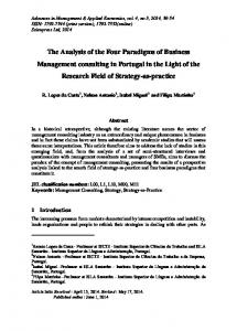
Figure 1: Graph showing Inverse Roots of VAR structure.
Umeh Edith Uzoma and Anazoba Uchenna Florence
25
Interpretation: Figure 1 shows the inverse roots of the characteristic AR polynomial; Lütkepohl (2005) and Hamilton (1994) both show that if the modulus of the eigenvalues of the matrix is strictly less than one and the roots lie inside the unit circle, the estimated VAR is stable. We were able to get roots for AR (1) and AR (2), since AR (3) and so on, appear invalid. If a root is real, it will lie on the horizontal axis; but if it is complex, if will be located at the point (x, y). Since no root lies outside the unit circle and the modulus is less than one, VAR satisfies the stability condition.
Markov-switching Regression Analysis
Table 3: Results of the analysis Coefficient
Std. Error
z-Statistic
Prob.
0.215595
0.8293
Regime 1 C
29.65635
137.5556 Regime 2
C
11001.54
851.1930
12.92485
0.0000
AR(1)
0.206507
0.050999
4.049275
0.0001
AR(2)
0.310993
0.051094
6.086679
0.0000
LOG(SIGMA)
7.134001
0.037689
189.2863
0.0000
Common coefficients
26
Application of Markov-Switching Regression Model on Economic Variables
Table 4: Transition matrix parameters P11-C
5.179004
0.716148
7.231750
0.0000
P21-C
8.956865
62.86110
0.142487
0.8867
Mean dependent var
96.22813
S.D. dependent var
S.E. of regression
1465.945
Sum squared resid
7.61E+08
Durbin-Watson stat
2.306951
Log likelihood
-3082.869
Akaike info
17.21376
Schwarz criterion
1562.039
17.28948
criterion Hannan-Quinn
17.24387
criter. Inverted AR Roots
0 .67
-0.46
Source: Authors computation. We see, from the upper part of table 3 the differences in the regime specific means (Regime 1: 29.65635, Regime 2: 11001.54), what Hamilton (1990) termed the fast and slow (in this case, the slow and fast) growth rates for the Nigeria stock market price for the period under study (1985 – 2014). We can also observe that regime 2 is significant (p0.05). This implies that the dynamics in the first regime is not substantial. The bottom section of table 4 shows the standard descriptive statistics for the equation. The unit roots are 0.67 and -0.46 which are real roots which means that they do not appear in conjugate pairs, they are roots on x-axis.
Estimation equation: 1: Diff = 29.6563463707 + [AR(1)=0.20650713911, AR(2)=0.310992536816]
2: Diff = 11001.5405593 + [AR(1)=0.20650713911, AR(2)=0.310992536816]
Umeh Edith Uzoma and Anazoba Uchenna Florence
27
where Diff = Differenced Data
Table 5: Transition probability 1
2
1
0.994398
0.005602
2
0.999871
0.000129
Expected durations: 1 178.5060
2 1.000129
Here, we see the transition probability matrix and the expected durations. The Transition probability is generated from the analysis run with E-views Statistical software version 9. The time-varying probabilities show considerable state dependence in the transition probabilities with a relatively higher probability of remaining in the origin regime, p (𝑠𝑡 =1| 𝑠𝑡−1 =1) is 0.994398 for the high output state and p (𝑠𝑡 =2| 𝑠𝑡−1 =2) is 0.000129 for the low output state. The corresponding expected
durations in a regime are approximately 178.5 and 1.0 quarters, respectively,
which imply that the stock market will remain in the origin state for a very long time before moving to the second state. Figure 2 displays the filtered estimates of the probabilities of being in the two regimes. Filtering is the process by which the probability estimates are updated. This is done in order to determine the likelihood of moving from one state to the other. This shows that the states are in the years 2008 and 2009.
28
Application of Markov-Switching Regression Model on Economic Variables
Filtered Regime Probabilities P(S(t)= 1) 1.0
0.8
0.6
0.4
0.2
0.0 1985
1990
1995
2000
2005
2010
2005
2010
P(S(t)= 2) 1.0
0.8
0.6
0.4
0.2
0.0 1985
1990
1995
2000
Figure 2: Chart showing the filtered estimates of the regime probabilities
4 Conclusions This study aimed at investigating regime switching in the stock market price using the Markov Switching Regression Model. Based on the results obtained from all the analyses, it concludes as follows; firstly, the study conclude that the Markov-Switching Regression model is a high-degree flexible model because it
Umeh Edith Uzoma and Anazoba Uchenna Florence
29
can capture regime shifts in the mean, in the variance and also the parameters of the vector autoregressive process. Secondly, it is found that the return series are well fitted by the MSVAR model and the filtered probabilities can be extracted. This is shown by the estimated parameters and the filtered probability plots of regime 1 and 2. Finally, it concludes that there is regime switching structure in the series.
References [1] A.O. Olufisayo, The Relationship between Changes in Oil prices and Stock Market in Nigeria, European Journal of Sustainable Development, 3(2), (2014), 33-40. [2] C.M. Kuan, Lecture on the Markov switching models, Institute of Economics, Academia Sinica, Taipei 115, Taiwan, (2002). [3] F.X. Diebold, J.H. Lee and G.C. Weinbach, Regime Switching with Timevarying Transition Probabilities, In C.P. Hargreaves editor, Non stationary Time Series and co integration, Oxford University press, (1994), 283-302. [4] H. Lütkepohl, New Introduction to Multiple Time Series Analysis, SpringerVerlag, Berlin, 2005. [5] H.K. Suleiman, Stock return and the Volatility Persistence in the Nigerian Capital Market, Seminal Paper, Department of Accounting, Ahmed Bello University, Zaria, (2011). [6] H.M. Krolzig, Construction of Turning Point Chronologies with Markovswitching Autoregressive models: the Euro-zone business cycle, Department of Economics and Nuffield College, Oxford University, 2003. [7] J.D. Hamilton , A New Approach to the Economic Analysis of Non stationary Time Series and the Business Cycle, Econometrica, 57(2), (1989), 357-384.
30
Application of Markov-Switching Regression Model on Economic Variables
[8] J.D. Hamilton, Analysis of Time Series Subject to Changes in Regime, Econometrica, 45, (1990), 39-70. [9] J.D. Hamilton, Time Series Analysis, Princeton University press, 1994. [10] M.T. Ismail and Z.B. Isa, Modeling Non-linear Relationship among Selected ASEAN Stock Markets, Data science, (2008), 533-545. [11] Nigeria Stock Exchange website. [12] O.O. Ifuero and I.E. Asein, Market Risk and Returns: Evidence from the Nigerian capital market, Asian Business Management, 4(4), (2012), 367-372.