Application of Maxeler Dataflow Supercomputing to Spherical Code Design Ivan Stanojevi´c, Mladen Kovaˇcevi´c, and Vojin Šenk
Abstract An algorithm for spherical code design, based on the variable repulsion force method is presented. The iterative nature of the algorithm and the large number of operations it performs make it suitable for implementation on dataflow supercomputing devices. Gains in computation speed and power consumption of such an implementation are given. Achieved minimum distances and simulated error probabilities of obtained codes are presented. Key words: Dataflow computing, high performance computing, spherical codes
1 Introduction A spherical code is a set of N D-dimensional real vectors on the unit sphere. Two standard optimization problems are associated with spherical codes: • given N and D, find a spherical code such that the minimum Euclidean distance between any two code vectors is maximized over the set of all such codes (packing problem); • given N and D, find a spherical code such that the radius of equally sized balls centered at code vectors and whose union contains the unit sphere, is minimized over the set of all such codes (covering problem). Ivan Stanojevi´c University of Novi Sad, Faculty of Engineering (a.k.a. Faculty of Technical Sciences), Serbia e-mail:
[email protected] Mladen Kovaˇcevi´c Department of Electrical and Computer Engineering, National University of Singapore e-mail:
[email protected] Vojin Šenk University of Novi Sad, Faculty of Engineering (a.k.a. Faculty of Technical Sciences), Serbia e-mail:
[email protected]
1
2
Ivan Stanojevi´c, Mladen Kovaˇcevi´c, and Vojin Šenk
Here, only the first problem will be addressed. The design of spherical codes is both an interesting theoretical and practical problem. There are only a few cases in which the exact solution is known [1], [5]. Good spherical codes can be used both for source coding [9] and channel coding [8], [20], as illustrated in Fig. 1. By increasing the minimum distance of the code
n . x
y
dmin Fig. 1 Spherical code used as a channel code, y = x + n (x - transmitted vector, n - noise vector, y - received vector); the minimum noise amplitude, |n|, which can produce an error is dmin /2
while keeping the number of vectors and their length fixed, noise resilience of the code is improved, for the same transmitted energy per symbol (vector) and the same code rate. For other interesting properties of spherical codes see also [6] (universal optimality), [7] (rigidity), and [21] (exact description using algebraic numbers). Dataflow supercomputing implemented on Maxeler systems is a new computing paradigm, which allows more time and energy efficient implementations of algorithms that are inherently parallelizable. The main idea is translation of the code that performs an algorithm into a dataflow structure in which streams of data are exchanged between simple processing blocks of programmable logic. If the number of operations that can be performed at the same time is high, acceleration can be achieved by using space multiplexing in an FPGA circuit, for which the host machine only provides input data and collects its output. There are several distinctive differences between dataflow acceleration and other competing technologies such as simultaneous execution of multiple threads on multicore central processing units (CPUs) or many-core processing units (most well known representatives of which are general-purpose graphics processing units or GPGPUs), together termed control flow systems:
Application of Maxeler Dataflow Supercomputing to Spherical Code Design
3
• In the dataflow approach, the most expensive part of the algorithm (in terms of the number of operations) is directly mapped into the corresponding dataflow structure, with a very deep pipeline (typically several thousand stages, limited only by the available resources of the FPGA), in which all the operations are executed every cycle. Unlike in control flow systems, there is no “instruction execution” (fetching an instruction opcode from memory, decoding it, fetching the operands and storing the result to memory). Movement of data is minimized by feeding all the intermediate results directly into blocks which need them as inputs, thus eliminating memory as a possible bottleneck. • Instead of minimizing latency, the aim of dataflow systems is maximizing data throughput. Scientific calculations most often require a large number of identical operations on input data and in such cases hardware resources are used efficiently in the deep pipeline, since except for the transient periods (initial filling of the pipeline and flushing it at the end) all the processing in it is done once every cycle, as its different stages act on different data. • In dataflow systems, the programmer has complete control over the processing in the FPGA (which operation is done in which block and how the blocks are interconnected), including its exact timing. This is not the case in multicore/manycore systems, in which the runtime environment (the operating system scheduler in multicore systems, or the execution framework, such as OpenCL or CUDA, in many-core systems) assigns portions of code to be executed to different processor cores. Although the latter approach adds flexibility and simplifies programming, as it makes execution of the same code possible with different numbers of cores, it is usually not optimum, since the automatic assignment algorithm is unaware of the problem being solved and can introduce unpredictable delays due to data dependencies, which can be hand-optimized in dataflow systems. • Control flow systems have a limited set of built-in number types, usually 8-, 16-, 32- or 64-bit integers/fixed-point numbers and 32- or 64-bit floating-point numbers. The programmer must use the “smallest” number type, large enough to hold values of a variable. This may use hardware inefficiently and increase the power consumption, as it may be possible to store values form the same range in a number type with a smaller number of bits. Since dataflow systems allow the processing structure to be defined at the level of logical units (e.g., flip-flops and logical functions), the minimum numbers of bits can be allocated for every variable, depending on the necessary value ranges. Maxeler library facilitates conversion between different number types in a design by built-in conversion substructures.
4
Ivan Stanojevi´c, Mladen Kovaˇcevi´c, and Vojin Šenk
2 Optimization Methods 2.1 Direct Optimization The optimization problem corresponding to optimal spherical code design can be formulated as follows: find D-dimensional vectors {r1 , r2 , . . . , rN } lying on the unit sphere, |ri | = 1, such that the cost function U = − min |r j − ri | i̸= j
(1)
attains its minimum value. A usual procedure for finding the minimum of a function like this one is to create an initial set of vectors and iteratively adjust every one of them until a minimum is reached. Although this optimization would produce a desired code, algorithms that perform it suffer from serious practical problems [15]. Since U only depends on the smallest distance between any two vectors, it locally depends only on the code vectors which have their nearest neighbours at the current minimum distance. If vectors are moved in the direction away from their nearest neighbours in every iteration, it is difficult to choose the length of those moves. Since the minimum distance should be increased at every move, when a vector has two or more neighbours at approximately the same minimum distance, the length of its move may be only very small, leading to extremely slow convergence. Another problem is that U is not differentiable with respect to vector coordinates, so the gradient descent method or Newton’s method cannot be applied directly to its minimization.
2.2 Variable Repulsion Force Method A different approach, successfully used in the literature [5], [10], [11], [12], [13], [14], and in this work, is to choose the differentiable cost function (assuming no vectors overlap) C V =∑ , (2) |r − ri |β −2 i< j j where C > 0 is an arbitrary constant and β > 2 is an adjustable parameter. V can be thought of as the potential of N particles repelling by the conservative central force (from the ith to the jth) ) ( r j − ri C △ Fi→ j = −∇r j = C(β − 2) . (3) β −2 |r j − ri | |r j − ri |β As β is increased, the force other particles exert on one particle starts to be dominated by the force of its nearest neighbours. If β → ∞, the force equilibrium (the
Application of Maxeler Dataflow Supercomputing to Spherical Code Design
5
stationary point of V ) is attained at a position where any particle has two or more nearest neighbours at an equal distance which is as large as possible. In such a position, the force exerted on the jth particle only has the component normal to the surface of the unit sphere, i.e., collinear with r j . Iterative minimization of V usually produces only a local minimum, and there is no guarantee that it is also a global minimum. In order to approach a global minimum as closely as possible, the procedure must be repeated multiple times with different initial vectors, which can be chosen at random. Since it is desirable that all randomly chosen points on the unit sphere be equally probable, i.e., that no directions be privileged, a simple two step procedure is used [15]: 1. choose coordinates g∗i,1 , . . . , g∗i,D as independent samples of a normalized Gaussian random variable (N (0, 1)); 2. normalize the obtained vector, ri =
g∗i . |g∗i |
(4)
For a fixed value of β , V can be minimized using the gradient descent method or Newton’s method. Even though Newton’s method has a faster rate of convergence, the gradient descent method is chosen here for the following reasons: • The overall solution of the problem is not the minimum of V for a particular value of β , but for β as high as possible, so β must be gradually increased after every iteration. The number of iterations which produce the minimum for a fixed β is irrelevant, since after β is increased the minimization is restarted (with a better initial position). • Gradient descent is much simpler and a single iteration is much faster. The negative partial gradient of V with respect to the jth vector is −∇r j V =
△
∑
Fi→ j = F→ j ,
(5)
i∈{1,...,N}\{ j}
which is the total force exerted on the jth particle. In order to preserve the constraint that all vectors are on the unit sphere, their new values can be calculated by moving them along the directions of the corresponding total forces and normalizing them, r∗j = r j + α F→ j , r j :=
r∗j |r∗j |
.
(6) (7)
The constant α > 0 determines the speed of the procedure and should be chosen so that the procedure is stable (vectors converge) and the error (the difference between the current and the final values) diminishes as fast as possible.
6
Ivan Stanojevi´c, Mladen Kovaˇcevi´c, and Vojin Šenk
Although α could be optimized to achieve the previous goals, when β is high enough the iteration in (6) and (7) suffers from numerical difficulties in a finite precision implementation: • if for some j, |r j − ri | > 1 for all i ̸= j, |r j − ri |−β can be calculated as 0 in (3) due to numerical underflow and F→ j can be calculated as 0 as well; • if for some i and j, |r j − ri | < 1, the calculation of |r j − ri |−β in (3) can cause numerical overflow. The likelihood of these conditions increases as β increases. In order to avoid these problems, a slight modification of the procedure will be used. Since every vector is moved along the direction of the corresponding force, that direction can be calculated by first scaling the force and then normalizing it. A convenient way to scale the force is )β /2 ( µj ∗ F→ j = (r j − ri ), (8) ∑ |r j − ri |2 i∈{1,...,N}\{ j} where
µj =
min
i∈{1,...,N}\{ j}
|r j − ri |2 .
(9)
The value of the subexpression in the first parentheses in (8) is in (0, 1] for all i, and is equal to 1 for at least one term, so neither underflow nor overflow can occur in the calculation of (8). The normalized force F∗→ j (10) F→ j = ∗ |F→ j | is used in a modified version of (6), r∗j = r j + α j F→ j , where
αj =
µj . 2β
(11)
(12)
It is shown in the appendix that this value of the step size, α j , ensures the stability of the process and fast convergence.
2.3 Force Loosening In order to maximize the minimum distance, β should be as high as possible. If vectors are moved with a high β immediately from their random initial position, the convergence is slow and the obtained local minimum of V usually produces a lower minimum distance than if β is gradually increased (the force gradually loosened). Given r1 , . . . , rN and β , the total move norm of one iteration,
Application of Maxeler Dataflow Supercomputing to Spherical Code Design
S = ∑ |r′j − r j |2 ,
7
(13)
j
can be calculated (r′1 , . . . , r′N are new vectors). It is observed in numerical results that for a continuous chain of iterations from a starting set of vectors and for fixed β , S decreases asymptotically exponentially with the number of iterations. It is also observed that if β is increased by the same amount after each iteration (linearly), after a transient period S starts decreasing as S ∼ β −1 . In order to reach high values of β quickly, yet without forcing the vectors into a position of numerical deadlock (which happens whenever β is increased too rapidly), the following strategy for increasing it is used: 1. Set n := 1 and l := 2. 2. Starting from r1 , . . . , rN and using β = 2l , calculate new vectors r′1 , . . . , r′N and the corresponding total move norm S′ . 3. Starting from r1 , . . . , rN and using β = 2l(1+1/n) , calculate new vectors r′′1 , . . . , r′′N and the corresponding total move norm S′′ . 4. If S′ > S′′ , set r j := r′j for all j. Otherwise, set r j := r′′j for all j and set l := l(1 + 1/n). 5. If more iterations are necessary, set n := n + 1 and go to step 2.
3 Implementation The majority of operations in the iterative procedure is performed in the loop for calculating new vectors. This is the part in which a number of operations can be done at the same time and can thus benefit from hardware acceleration. For convenience, an overview of steps performed for a single vector is given here: 1. µ j = mini∈{1,...,N}\{ j} |r j − ri |2 . ( )β /2 µ (r j − ri ). 2. F∗→ j = ∑i∈{1,...,N}\{ j} |r −rj |2 j i F∗→ j |F∗→ j | . µ r∗j = r j + 2βj F→ j . r∗ r j := |r∗j | . j
3. F→ j = 4. 5.
The new vector, calculated in the last step, can be stored: • in the same memory location as the old one, which is more convenient for a software implementation, since only one block of memory is used; • in the appropriate location of a different block of memory or another data stream, which is more convenient for a streamed hardware implementation, since it simplifies dependencies on input data. Although the new values obtained in these ways differ, they can both be successfully used for finding good spherical codes.
8
Ivan Stanojevi´c, Mladen Kovaˇcevi´c, and Vojin Šenk
3.1 Software Implementation In the software implementation, vector coordinates are stored as floating-point numbers. Operations with them are performed by the floating-point unit (FPU) of the CPU and by the runtime library functions, which are highly optimized. Their data type is the standard IEEE 754 double precision type [22], with 53 bits of mantissa and 11 bits of exponent. Since vector coordinates and vectors themselves are accessed sequentially in all the operations performed on them, the algorithm has good cache locality. Typically, for codes used in practice, values N and D are such that the total amount of iterated data is small enough to fit completely in the cache of modern processors.
3.2 Hardware Implementation In the hardware implementation, vector coordinates are stored as signed fixed-point numbers with 3 integer bits and 44 fractional bits. Maxeler dataflow engines support highly configurable number formats and this choice is the result of the following limitations: • Vector coordinates are in the interval [−1, 1], their differences are in [−2, 2] and their squares are in [0, 4], so at least 3 integer bits are necessary. • Some Maxeler library functions (e.g., for calculating square roots) have an upper bound on the total number of bits of fixed-point numbers they can operate on. Since other fixed-point types with a higher number of integer bits are used for storing intermediate results, a total of 47 bits is obtained as the highest value for which all the calculations can be performed using only library functions. Although floating-point numbers can be used as well, fixed-point numbers occupy much less hardware resources. Operations on vectors, such as addition (subtraction), multiplication (division) by a scalar or norm calculation are performed in parallel on all their coordinates, as shown in Figs. 2-4. Although it may seem that these calculation structures yield their results instantaneously, it is not the case, since each of them introduces a pipeline delay of several cycles, which depends on used number types and low-level compiler decisions. This delay only increases the overall (long) pipeline delay, i.e., the time from the moment when the first input data block enters the dataflow structure until the first result block can be read at its output, which is added to the total calculation time only once (not once for every block of input data). If the number of cycles needed to perform all the calculations is much larger than the pipeline delay, that delay can be neglected, and it can be considered that all the operations in the structure are done in parallel, once every cycle. In the algorithm above, µ j , which is calculated in step 1, is used in steps 2-5. In the software implementation two separate inner loops over i are necessary in steps 1 and 2. Whereas this is also the case in the hardware implementation, another level of
Application of Maxeler Dataflow Supercomputing to Spherical Code Design a1
a2
aD
b1
.
9
b2
bD
+ +
+
c1
c2
cD
Fig. 2 Dataflow substructure for parallel addition of vectors a1
a2
aD
b
. · ·
·
c1
c2
cD
Fig. 3 Dataflow substructure for parallel multiplication of a vector and a scalar
parallelism is possible: while µ j is being used in steps 2-5, µ j+1 can be calculated, as shown in Fig. 5. Since one inner loop (for calculating a single value of µ j or r j ) lasts N cycles, one complete iteration lasts N(N + 1) cycles. The maximum number of vectors, Nmax , and their maximum dimension, Dmax , must be hard coded in the dataflow structure. In order to provide a flexible solution, the actual number and dimension of vectors, N and D, are configured as run-time parameters (scalar inputs). On a Maxeler MAX21 device, possible values are Nmax = 16384 and Dmax = 6. These values are obtained by fine tuning the design, since MAX2 is a PCI Express expansion card with a ×8×8 interface. It has two Xilinx Virtex-5 LX330T FPGAs operating at 100MHz, each connected to 6GB of DDR2 SDRAM.
1
10
Ivan Stanojevi´c, Mladen Kovaˇcevi´c, and Vojin Šenk a1
a2
aD
()2
()2
()2
.
+
√ ()
|a| Fig. 4 Dataflow substructure for calculation of the (squared) norm of a vector
µ1 r1
µ2 r2
µ3 r3
µ4 .. .
↓ time ↓
..
. rN−1
µN rN
Fig. 5 Order of calculation: dependent values are in the same columns, and independent values calculated at the same time are in the same rows
FPGA circuits have a limited number of programmable logic elements: look-up tables (LUTs), flip-flops (FFs), block RAM modules (BRAMs) and digital signal processing modules (DSPs). The actual resource usage is shown in Table 1. Table 1 MAX2 FPGA Resource Usage LUTs FFs BRAMs DSPs
Used 157716 193082 225 141
Maximum 207360 207360 324 192
Percentage 76.06% 93.11% 69.44% 73.44%
The architecture of the system is shown in Fig. 6. The host application is responsible for creating the initial vectors, sending the current vectors in each iteration to the dataflow device and collecting their updated values. Vector coordinates are transferred serially from the host and back to the host. On the dataflow device, they are internally converted to the parallel form in the serial-to-parallel (S/P) converter and
Application of Maxeler Dataflow Supercomputing to Spherical Code Design
11
S/P converter
Host application
Vector updater
P/S converter . Fig. 6 Architecture of the system: blocks inside the dashed box are on the Maxeler MAX2 dataflow device
after the update back to the serial form in the parallel-to-serial (P/S) converter. Both conversions last ND cycles, but since outputs of each block are available before its execution ends, the total execution time of one iteration is less than 2ND + N(N + 1) cycles.
3.3 Performance Measured execution times of a single iteration are shown in Fig. 7. The host CPU is Intel
[email protected] and the software implementation is single-threaded, executing in 64-bit mode. The host operating system is Linux (distribution CentOS 6.4, kernel version 2.6.32-358.18.1). During the measurements, all motherboard functions which change the CPU clock frequency depending on the load are disabled. For low values of N, the software implementation is considerably faster than the hardware one, since in the latter case the majority of time is spent on the communication between the host and the dataflow device. For N ≳ 50, the hardware implementation becomes faster than the software one despite all the overhead of communication and control the host needs to perform. For N ≳ 500, the execution time of the hardware implementation starts to show similar asymptotic behaviour as that of the software one, since it is dominated by the actual calculations. Both procedures are essentially the same and quadratic in N. It is interesting to note that the time of execution in software increases as the vector dimension, D, increases, but is not proportional to it. This can be explained by the time needed for other operations apart from vector operations. In hardware, the times for different values of D are practically the same (their curves in Fig. 7 almost overlap) since vector operations are done in parallel. Their only small differences are caused by different amounts of data exchanged between the host and the dataflow engine, but those are within measurement errors.
12
Ivan Stanojevi´c, Mladen Kovaˇcevi´c, and Vojin Šenk
101
Single iteration time (s)
. 100 10−1 10−2 10−3 10−4 10−5 10−6 . 101
102 Number of vectors
103
104
Fig. 7 Execution times, N ∈ [4, 8192] and D ∈ [3, 6]: results for the software implementation are shown in dashed lines and for the hardware implementation in solid lines
The asymptotic speed gains of hardware acceleration are approximately (18 ÷ 24)×, for D ∈ [3, 6]. Figures 8 and 9 show FPGA device usage and temperature obtained by the maxtop utility, with ambient temperature of 23◦ C. FPGA device temperature in idle mode is 45.5◦ C. Power consumption of the host in different execution modes is shown in Table 2. The measurements are performed on the mains cable of the host, with an estimated Table 2 Host Power Consumption Mode Idle Software execution Hardware execution
Power (W) 68 88 74
relative error of 5%. Although the majority of power is used for idle operation of the host, which includes power for its auxiliary devices such as hard disks and fans, additional con-
Application of Maxeler Dataflow Supercomputing to Spherical Code Design
13
100
FPGA device usage (%)
80
60
40
20
.
0.
101
102 Number of vectors
103
104
Fig. 8 FPGA device usage, N ∈ [4, 8192] and D = 6
sumption for hardware execution is lower than for software execution, even when only a single thread is active.
4 Results 4.1 Minimum Distances Minimum distances of spherical codes obtained by taking the best of 32 optimizer runs for different N and D are shown in Fig. 10. Even though these results are not the absolute optimum values, they are very close to them (the reader is referred to online tables compiled by Sloane [23] for a detailed list of the best known and other interesting spherical codes), and can serve as a starting point for calculating possible coding gains in systems which employ the constructed codes.
14
Ivan Stanojevi´c, Mladen Kovaˇcevi´c, and Vojin Šenk
FPGA device temperature (◦ C)
51
50
49
48
47
. 46 . 101
102 Number of vectors
103
104
Fig. 9 FPGA device temperature, N ∈ [4, 8192] and D = 6
4.2 Code Performance Simulated frame error probabilities of some spherical codes are shown in Figs. 1114. Optimum decoding is performed for the channel with additive white Gaussian noise, with signal/noise ratio SNR = 10 log
1/D , σ2
(14)
where σ is the variance of noise per real dimension. Since all codewords are of unit energy, the energy per transmitted symbol is 1/D. In all figures, solid lines represent the simulated code performance, and dashed lines represent the performance of hypercube and [ codes ] √ with the same √ dimension number of symbols, whose codewords are ±1/ D · · · ±1/ D , which correspond to uncoded binary transmission. In the latter case, frame error probability can be calculated as Pf = 1 − (1 − Ps )D , (15) where
Application of Maxeler Dataflow Supercomputing to Spherical Code Design
15
1.6 1.4
Minimum distance
1.2 1 0.8 0.6 0.4 0.2 0. 0
20
40
60
80
100 120 140 160 Number of vectors
180
200
220
240
Fig. 10 Minimum distances of spherical codes: achieved minimum distances of obtained codes for D = 3, 4, 5, 6 (from bottom to top) are shown in solid lines and minimum distances of the best known spherical codes for D = 3, 4, 5 (from Sloane’s tables) are shown in dashed lines
( ) 1 Ps = Q √ Dσ
(16)
is the symbol error probability, and 1 Q(x) = √ 2π
∫∞
t2
e− 2 dt.
(17)
x
For high SNR’s, error probability is dominated by the code minimum distance, which determines the asymptotic coding gain of spherical codes
∆ SNR = 20 log
dmin √ , 2/ D
(18)
√ where dmin is the minimum distance of a spherical code, and 2/ D is the minimum distance of the corresponding hypercube code. Achieved coding gains for the simulated codes are shown in Table 3.
16
Ivan Stanojevi´c, Mladen Kovaˇcevi´c, and Vojin Šenk 100 .
10−1
Pf
10−2
10−3
10−4
10−5 . −4
−2
0
2
4
6 SNR (dB)
8
10
12
14
Fig. 11 Frame error probability, D = 3, N = 8 Table 3 Coding Gains D 3 4 5 6
N 8 16 32 64
dmin 1.216 1.107 1.056 0.989
∆ SNR (dB) 0.45 0.88 1.45 1.66
5 Methodology Considerations In [2] an interesting classification of different approaches to generation of new ideas for PhD research in computing is given, without purporting that the list of 10 different methods covers all possible cases. According to that list, we used the following methods: • Extraparametrization Instead of solving the original problem of minimizing the “hard potential” cost function (1), a different “soft potential” cost function (2) is minimized, which depends on a new parameter, β . As explained in section 2, this ensures the nu-
Application of Maxeler Dataflow Supercomputing to Spherical Code Design
17
100 .
10−1
Pf
10−2
10−3
10−4
10−5 . −4
−2
0
2
4
6 SNR (dB)
8
10
12
14
Fig. 12 Frame error probability, D = 4, N = 16
merical stability of the procedure and enables the use of general optimization methods, which require differentiable cost functions. • Transgranularization Even though the solutions of the two problems are in general different for any finite value of β , by carefully increasing it, the sequence of vector positions obtained while solving the second problem can be made arbitrarily close to a local optimum of the first problem. The procedure for this, described in subsection 2.3, is a novelty of the present method. Unlike in previous approaches, e.g., [10], [11], [12], [13], [14], [21], where β was kept fixed or increased in discrete steps after numerical convergence, continuous adaptation of β is equivalent to its finegrained control and it results in a lower number of iterations and faster convergence. • Revitalization Advances in high performance computing and the development of the dataflow computing paradigm revitalized the problem, which was being solved by traditional methods during the last three decades. This broadened the range of parameters N and D for which solutions can be obtained and increased the precision of those solutions.
18
Ivan Stanojevi´c, Mladen Kovaˇcevi´c, and Vojin Šenk 100 .
10−1
Pf
10−2
10−3
10−4
10−5 . −4
−2
0
2
4
6 SNR (dB)
8
10
12
14
Fig. 13 Frame error probability, D = 5, N = 32
In general, there are numerous methodologies for generating ideas, to name a few: brainstorming [17], lateral thinking [4], mind mapping [3], and TRIZ [16], [18], [19]. The last one focuses more on techniques of problem solving than on psychological aids to achieve the intellectual freedom necessary to solve problems (the so-called “thinking outside the box”), so we will focus on it here. Although rather elaborate and complicated to understand and apply, it is based on millions of studied patents and it yielded a list of 40 principles from mechanical engineering that can, in a broader sense, be applied to all areas of engineering in order to yield efficient solutions to nonstandard problems. From the list of 40 TRIZ principles, the following ones can be identified: • Nonlinearity (standard name: Spheroidality - Curvature) The solutions to the problem are confined to a D-dimensional sphere, and its curvature enforces nonlinearities that are tackled by minimizing a nonlinear potential cost function. • Dynamics The parameter of the cost function, β , is dynamically changed according to the estimated speed of convergence to the solution to the initial problem (subsection 2.3).
Application of Maxeler Dataflow Supercomputing to Spherical Code Design
19
100 .
10−1
Pf
10−2
10−3
10−4
10−5 . −4
−2
0
2
4
6 SNR (dB)
8
10
12
14
Fig. 14 Frame error probability, D = 6, N = 64
• Partial, overdone or excessive action The optimization is not completed for any finite value of β . Rather, β is increased as soon as that is estimated to be beneficial for faster convergence to the final solution. • Feedback The decision whether to increase β or not is made by calculating the move norm (13) of both options in every iteration. • Parameter change The gradient descent step size (12) is calculated for every particle being moved in order to ensure convergence. • Cheap short-living objects For given N and D, a number of different initial sets of vectors are randomly generated and the procedure is run for every one of them. The results are obtained as the optimum of all the runs.
20
Ivan Stanojevi´c, Mladen Kovaˇcevi´c, and Vojin Šenk
Acknowledgement This work was supported by the Ministry of Education, Science and Technological Development of the Republic of Serbia, grant 451-03-00605/2012-16/198, project “Cloud Services for Applications with High Performance Requirements,” and grant III44003, project “Conflagration Detection and Estimation of its Development by means of an Integrated System for Real Time Monitoring of Critical Parameters.”
Appendix We intend to justify our choice of the parameter α (see (12)), since it has been observed experimentally that: • this choice ensures the stability and convergence of the algorithm, • some other choices of α can lead to oscillatory behaviour, or very slow convergence. Here, we wish to give a formal argument of convergence when (12) holds by proving the following claim: If a particle is in a neighbourhood of a stable balance position2 , then the above algorithm will make it converge towards this position (all other particles being fixed). We will first analyze the case of infinitesimally small neighbourhoods. This analysis will enable us to obtain explicitly some relations needed for the finite neighbourhood case stated in Theorem 3.
Two-Dimensional Case We start with the case N = 3, D = 2, i.e., 3 particles on the unit circle. This simple example illustrates the main idea and makes the general case (analyzed in the following subsection) easier to follow. Also, it enables one to explicitly obtain the condition (12) which ensures convergence of the algorithm. Theorem 1. Let N = 3, D = 2. If one of the particles is in an infinitesimally small neighbourhood of a stable balance position, then the above algorithm will make it converge towards this position. Proof. Observe the configuration of points illustrated in Figure 15: [ ] m= 1 0 , [ ] r1 = cos γ sin γ , [ ] r2 = cos γ − sin γ .
(19)
2 We shall later give a precise definition of what is meant by a “stable balance position” of a particle.
Application of Maxeler Dataflow Supercomputing to Spherical Code Design
21
p1 + δ p1 t
p1
r1
F+δF m+δm .
δm
γ m
γ
F
p2 + δ p2 p2
r2
Fig. 15 Particle movement in the two-dimensional case
The particle m is in a stable balance position. The force exerted on this particle is (assuming for convenience C = 1/(β − 2)) F=∑ i
pi m − ri =∑ , β β |m − ri | i |pi |
(20)
where the vectors pi = m − ri determine the position of the observed particle with respect to the remaining particles. They are introduced primarily to simplify notation. We have [ ] p1 = 1 − cos γ − sin γ , [ ] p2 = 1 − cos γ sin γ , (21) γ |p1 | = |p2 | = 2 sin , 2 and by using some simple trigonometric identities we obtain ( γ )−β +2 F = 2 sin m. 2
(22)
22
Ivan Stanojevi´c, Mladen Kovaˇcevi´c, and Vojin Šenk
We need to show that, if the observed particle is in some neighbourhood of the stable balance position (m), then the presented algorithm will make it converge towards this position, provided that (12) holds. Assume that the particle is moved by an infinitesimally [ ] small amount along the circle δ m = δ m t, where δ m = |δ m|, and t = 0 1 is the tangent unit vector at m (see Figure 15). The vectors determining the position of this particle with respect to the other particles are now pi + δ pi = m + δ m − ri , i.e.: [ ] p1 + δ p1 = 1 − cos γ − sin γ + δ m , [ ] (23) p2 + δ p2 = 1 − cos γ sin γ + δ m . and hence, the force exerted on the particle at this position is |p1 + δ p1 |−β ·
F+δF =
+ |p2 + δ p2 |−β · where
[ [
1 − cos γ 1 − cos γ
− sin γ + δ m ] sin γ + δ m ,
] (24)
( )− β 2 |p1 + δ p1 |−β = (1 − cos γ )2 + (− sin γ + δ m)2 , −β
|p2 + δ p2 |
( )− β 2 = (1 − cos γ )2 + (sin γ + δ m)2 .
(25)
Note that, since δ m is an infinitesimally small quantity, any differentiable expression depending on δ m can be linearized by developing it into a Maclaurin series and disregarding all higher order terms f (δ m) ≈ f (δ m)
+ δ m=0
d f (δ m) dδ m
δ m=0
δ m.
(26)
By linearizing the right-hand sides of (25) in this way, we obtain ( )− β 2 (1 − cos γ )2 + (± sin γ + δ m)2 = ) ) ( ( γ −β γ −β −1 ( γ) cos = 2 sin ± β 2 sin δ m, 2 2 2 which, together with (24), gives [ ( )−β +2 F+δF = 2 sin 2γ
] ( γ )−β ( γ) 2 2 2 sin 2 1 − β cos 2 δ m .
(27)
(28)
We also have (again ignoring higher order infinitesimals) ( γ )−β +2 |F + δ F| = 2 sin = |F|. 2
(29)
Application of Maxeler Dataflow Supercomputing to Spherical Code Design
23
Therefore, if the particle finds itself at the position m + δ m, the force it will feel is given by (28). Recall that in this case the algorithm works as follows: We move the particle along the direction of the force and then project it back onto the circle. The direction of the force is determined by the vector [ F+δF = 1 |F + δ F| where G = δF |F| .
F |F|
1−β cos2 2γ 2 sin2 2γ
δm
]
= G + δ G,
(30)
= m is the normalized force at the stable balance position, and δ G =
We now need to move the particle for α (G + δ G), and then to project it onto the circle, i.e., normalize its radius vector. The new position is therefore m + δ m′ =
m + δ m + α (G + δ G) . |m + δ m + α (G + δ G)|
(31)
We have m + δ m + α (G + δ G) =
[
1+α
( ) ] 1−β cos2 γ 1 + α 2 sin2 γ 2 δ m
(32)
2
and |m + δ m + α (G + δ G)| = 1 + α , so that
m + δ m′ =
where b=
[
1
1+α b 1+α δ m
1 − β cos2 2γ 2 sin2 2γ
]
,
.
(33) (34)
(35)
Thus the new distance of the particle from the stable balance position (after the execution of one step of the algorithm) is 1 + αb δ m. δ m′ = |δ m′ | = (36) 1+α We would like this displacement to be as small as possible (δ m′ ≈ 0) so that the particle converges quickly to the stable balance position, but in general it is enough that 1 + αb (37) 1+α < 1 to ensure convergence. In other words, the optimal choice is α = −1 b . Unfortunately, expression (35) cannot be generalized to the higher-dimensional case in a straightforward way. We therefore find a simpler expression by lower bounding b, b>
−β cos2 2γ 2 sin2 2γ
>
−β −2β , = 2γ µ 2 sin 2
(38)
24
Ivan Stanojevi´c, Mladen Kovaˇcevi´c, and Vojin Šenk
where 2 µ = dmin ,
(39)
γ 2
and dmin = mini |pi | = 2 sin is the minimum Euclidean distance from the observed particle to any of the other particles. Now from α = −1 b , and by using the above bound instead of b, we get µ α= . (40) 2β It is easy to show that this value satisfies (37) for all β > 1, thus completing the proof of the claim.
General Case Let us now consider the general case with N particles on the D-dimensional unit sphere. The idea of the proof is the same as in the 2D case. Namely, we again observe a particle in a stable balance position m, and consider what happens if this particle is moved slightly in any direction. Definition 1. Let some configuration of particles be specified, and observe the particle at the point m. Let t be a unit vector in the tangent hyperplane at m. If the particle is moved by an infinitesimal amount in the direction of t, i.e., δ m = δ m t, the new tangent vector (lying in the plane defined by m and t) is t + δ t, and the force exerted on the particle is F + δ F. We say that m is a stable balance position for the observed particle if (F + δ F) · (t + δ t) < 0. (41) Intuitively, this condition means that the force pushes the particle back to m. See Fig. 16 for an illustration. It is easy to show that the above condition implies that F = |F|m, i.e., that the force exerted on the particle in a stable balance position is orthogonal to the surface of the sphere. Consequently, F · t = 0. We shall use these facts later. Let us now prove a generalization of Theorem 1. Theorem 2. Observe a configuration of N points on a D-dimensional sphere, and let one of the particles be in an infinitesimally small neighbourhood of a stable balance position. Then the above algorithm will make it converge towards this position. Proof. The force exerted on the observed particle located at m is F=∑ i
pi m − ri =∑ , β |m − ri |β |p i| i
(42)
where pi = m − ri , and the ri ’s are the positions of the other particles, as before. Since this is by assumption a stable balance position, we have F = |F|m. Assume now that the particle is displaced by δ m, i.e., that its new position is m + δ m. (For
Application of Maxeler Dataflow Supercomputing to Spherical Code Design
25
δt
t+δt
t
F+δF m+δm .
δm
m
F
Fig. 16 Particle movement in the general case
now we allow all directions of the displacement, i.e., we do not assume that δ m is tangential to the sphere at m.) Then its position relative to the particle ri is changed by δ pi = δ m. The force it feels at this position is F + δ F = ∑ |pi + δ pi |−β (pi + δ pi ) i
(43)
= ∑ |pi + δ m|−β (pi + δ m). i
We have
( )− β 2 |pi + δ m|−β = (pi + δ m) · (pi + δ m) − β2
= (pi · pi + 2pi · δ m)
(44)
,
where we have disregarded higher order infinitesimals, as usual. (We denote by x · y the inner product of vectors x and y. Note that, since we have adopted the row-vector notation, we could also write xyT for the inner product.) As in the proof of Theorem 1, we can linearize expressions depending on infinitesimally small quantities, but we now need the multivariate form, f (δ m) ≈ f (δ m) where δ m = obtain
[
δ m1
···
∂ f (δ m) u=1 ∂ δ mu D
δ m=0
+∑
δ m=0
δ mu ,
(45)
] δ mD . By linearizing expression (44) in this way, we
|pi + δ m|−β = |pi |−β − β |pi |−β −2 pi · δ m
(46)
26
Ivan Stanojevi´c, Mladen Kovaˇcevi´c, and Vojin Šenk
and hence the force can be expressed as ( ) F + δ F = ∑ |pi |−β − β |pi |−β −2 pi · δ m (pi + δ m) i
) ( = ∑ |pi |−β pi + |pi |−β δ m − β |pi |−β −2 (pi · δ m)pi ,
(47)
i
from which we conclude that the differential of the force at the stable balance position is ( ) δ F = ∑ |pi |−β δ m − β |pi |−β −2 (pi · δ m)pi i (48) = ∑ |pi |−β (δ m − β (qi · δ m)qi ) , i
where qi =
pi |pi | .
We further have ( )− 1 2 |F + δ F|−1 = (F + δ F) · (F + δ F) = (F · F + 2F · δ F)− 2
1
(49)
= |F|−1 − |F|−3 F · δ F, where the last expression is obtained by linearization, as before. Now, |F + δ F|−1 (F + δ F) = |F|−1 F + |F|−1 δ F − |F|−3 (F · δ F)F = G + δ G,
(50)
where G = |F|−1 F = m is the normalized force at the stable balance position, and δ G = |F|−1 δ F − |F|−1 (m · δ F)m. Notice that
δ G · m = |F|−1 δ F · m − |F|−1 (m · δ F)(m · m) = 0.
(51)
Now, the new position of the particle, after moving and projecting back onto the sphere, is m + δ m + α (G + δ G) m + δ m′ = |m + δ m + α (G + δ G)| (52) (1 + α )m + δ m + αδ G = . |(1 + α )m + δ m + αδ G| Let us calculate the new displacement δ m′ . Taking (51) into account, we have
Application of Maxeler Dataflow Supercomputing to Spherical Code Design
27
|(1 + α )m + δ m + αδ G|−1 = (( ) ( ))− 12 = (1 + α )m + δ m + αδ G · (1 + α )m + δ m + αδ G ( )− 1 2 = (1 + α )2 m · m + 2(1 + α )m · δ m )− 1 ( 2 = (1 + α )2 + 2(1 + α )m · δ m ,
(53)
which after linearization becomes |(1 + α )m + δ m + αδ G|−1 =
1 1 − m · δ m. 1 + α (1 + α )2
(54)
Plugging this back into (52) we get ( ) |(1 + α )m + δ m + αδ G|−1 (1 + α )m + δ m + αδ G = = m+
α 1 1 δm+ δG− (m · δ m)m. 1+α 1+α 1+α
(55)
It follows that the new distance (after the execution of one step of the algorithm) from the stable balance position is given by 1 α 1 δm+ δG− (m · δ m)m 1+α 1+α 1+α ) 1 α ( −1 = (δ m − (m · δ m)m) + |F| δ F − |F|−1 (m · δ F)m , 1+α 1+α
δ m′ =
(56)
or equivalently by
δ m′ =
1 (δ m − (m · δ m)m) 1+α ( α −1 + |F| ∑ |pi |−β (δ m − β (qi · δ m)qi ) 1+α i ) ) ( − m · ∑ |pi |−β (δ m − β (qi · δ m)qi ) m
(57)
i
=
1 δ mt 1+α ( ( )) α + |F|−1 ∑ |pi |−β δ mt − β (qi · δ m) qi − (qi · m)m . 1+α i
In equation (57) we have denoted by δ mt = δ m − (m · δ m)m the tangential component of the vector δ m (see Fig. 17), which can also be written as
δ mt = δ m(I − mT m),
(58)
28
Ivan Stanojevi´c, Mladen Kovaˇcevi´c, and Vojin Šenk
where I is the D × D identity matrix, and mT m is the D × D matrix of the projection operation (onto m). Observe from the figure that δ m can be decomposed as
t
δm
δ mt η
.
δ mm
m
Fig. 17 Particle displacement decomposition
δ m = δ m(cos η m + sin η t) = δ mm + δ mt ,
(59)
so we can write 1 δ mt 1+α ( ( )( )) α + |F|−1 ∑ |pi |−β δ mt − β qi · (δ mm + δ mt ) qi − (qi · m)m . 1+α i (60) From (60) we can deduce that δ m′ · m = 0, i.e., that the displacement δ m′ has only the tangential component, as expected (after projecting, the particle is displaced by an infinitesimal amount in the tangent hyperplane at the point m). Plugging (59) into (60) we obtain ( δm sin η t δ m′ = 1+α ( + α |F|−1 ∑ |pi |−β sin η t
δ m′ =
i
− β cos η (qi · m)qi
(61)
+ β cos η (qi · m)2 m − β sin η (qi · t)qi + β sin η (qi · t)(qi · m)m To simplify expression (61) recall that qi =
pi |pi | ,
)) .
and observe from Fig. 18 that
Application of Maxeler Dataflow Supercomputing to Spherical Code Design
γi |pi | = 2 sin , 2 (π γ ) γi |pi | i − = sin = . qi · m = |qi ||m| cos 2 2 2 2
29
(62)
We further have
pi
ri
γi 2
.
γi 2
m
Fig. 18 ri – m plane
∑ |pi |−β (qi · m)2 m = ∑ |pi |−β i
i
|pi | (qi · m)m 2
1 = ∑ |pi |−β (pi · m)m 2 i ( ) ) 1 ( −β = ∑ |pi | pi · m m 2 i
(63)
1 1 = (F · m)m = |F|m 2 2 1 = F, 2 and similarly 1
∑ |pi |−β (qi · t)(qi · m) = 2 F · t = 0,
(64)
i
and
1
∑ |pi |−β (qi · m)qi = 2 F. i
We now obtain
(65)
30
Ivan Stanojevi´c, Mladen Kovaˇcevi´c, and Vojin Šenk
δ m′ =
( ) ) δ m sin η ( 1 + α |F|−1 ∑ |pi |−β t − α |F|−1 β ∑ |pi |−β (qi · t)qi . (66) 1+α i i
This is a linear transformation, which can be written in the following form
δ m sin η t(I + α B) 1+α I + αB = δ mt 1+α I + αB = δ m(I − mT m) , 1+α
δ m′ =
(67)
where I is the identity matrix, and B = |F|−1 ∑ |pi |−β (I − β qiT qi ).
(68)
i
Here qiT qi is the matrix of the projection operation (onto qi ). It follows now from (67) that |δ m′ | ≤ |δ m| ∥J(m)∥ , (69) where J(m) = (I − mT m)
I + αB , 1+α
(70)
and ∥·∥ denotes the matrix norm (defined by ∥S∥ = max|u|=1 |uS|). Notice the similarity of (69) with the expression obtained in the two-dimensional case, (36). (The factor (I − mT m) which appears above is a consequence of δ m being arbitrary, not necessarily tangential as was assumed in the proof of Theorem 1. By (58), the vector δ m (I − mT m) is precisely the tangential component of δ m.) Now, to prove that the particle converges towards its stable balance position, i.e., that the displacement decreases in every step, we need to show that ∥J(m)∥ < 1. Note that the matrix J(m) is symmetric, and recall that the norm of a symmetric matrix is equal to its spectral radius, i.e., the largest absolute value of its eigenvalues. It can readily be shown (by using Cauchy-Schwartz inequality, for example) that the norm of a symmetric matrix S can also be expressed as ∥S∥ = max |uS · u|. |u|=1
(71)
Actually, in the case of J(m) the maximization can be done only over the unit vectors t orthogonal to m, i.e., vectors lying in the tangential hyperplane at m. This follows from the fact that the vectors uJ(m) have only tangential components, as is easily concluded from (66) and (64). Therefore, we can write ∥J(m)∥ =
max
|t|=1,t·m=0
|tJ(m) · t|.
(72)
Application of Maxeler Dataflow Supercomputing to Spherical Code Design
31
Observe that the quadratic form defining the norm of our matrix can be expressed as I + αB 1 + αb tJ(m) · t = t ·t = , (73) 1+α 1+α with ) ( b = |F|−1 ∑ |pi |−β 1 − β (qi · t)2 . (74) i
αb We therefore need to show that 1+ 1+α < 1. Recall that for δ m = δ m t we must have (F + δ F) · (t + δ t) < 0 because m is by assumption a stable balance position. This can further be written as (F + δ F) · (t + δ t) = F · δ t + δ F · t
( ) = F · (−δ m)m + δ m ∑ |pi |−β t − β (qi · t)qi · t i
( ) = −δ m|F| + δ m ∑ |pi |−β 1 − β (qi · t)2
(75)
i
( )) ( = δ m|F| − 1 + |F|−1 ∑ |pi |−β 1 − β (qi · t)2 < 0, i
where we have used the following facts: F · t = 0, δ t = −δ m m (see Fig. 16), and δ F · δ t is disregarded as a higher order infinitesimal. The condition for the particle being in a stable balance position is therefore equivalent to ) ( (76) |F|−1 ∑ |pi |−β 1 − β (qi · t)2 < 1. i
The left-hand side of (76) is precisely b (see (74)) and hence we have shown that αb 1+α b b < 1, which further implies that 1+ 1+α < 1. It is left to prove that also 1+α > −1. Observe that b ≥ |F|−1 ∑ |pi |−β (1 − β ) (77) i
because qi · t ≤ 1. Also, we have |F| = F · m = ∑ |pi |−β pi · m = i
1 |pi |−β |pi |2 , 2∑ i
(78)
where the last equality follows from (62). From (77) and (78) (and the fact that 1 − β < 0) we now get ∑i |pi |−β −β |p |2 i 2 ∑i |pi |
b ≥ (1 − β ) 1
∑i |pi |−β −β min |p |2 k k 2 ∑i |pi | 2 = (1 − β ) , µ ≥ (1 − β ) 1
(79)
32
Ivan Stanojevi´c, Mladen Kovaˇcevi´c, and Vojin Šenk
where
µ = min |pi |2 i
(80)
is the squared minimum distance from the observed particle to any of the other particles, as already introduced in (39). We now finally obtain (recall that the parameter of the algorithm α is defined as 2µβ )
µ µ 2 b≥ (1 − β ) > −1, (81) 2β 2β µ αb > −1. We have thus shown that 1+ 1+α < 1, and consequently αb =
which implies (see (73)) that
1+α b 1+α
∥J(m)∥ < 1.
(82)
This, as we have already discussed (see (69)), means that the particle converges to a stable balance position according to our algorithm whenever it finds itself in an infinitesimal neighbourhood of such a position. We now wish to extend the above result to the case of a finite neighbourhood of a single particle. A couple of definitions are needed first. of m we By an ε -neighbourhood { } will understand an open ball around m of radius ε , i.e., x ∈ RD : |x − m| < ε . In the following proof, we will assume that the particle’s initial position is in some neighbourhood of a stable balance position, and consequently, that it is not necessarily on the sphere. This assumption yields a slightly more general claim than is needed, but actually simplifies the proof. Assume that the observed particle is located at x and one step of the algorithm is executed. We can define a mapping f such that f(x) represents the new position of the particle after the execution of one step of the algorithm, assuming that the positions of the remaining N − 1 particles are kept fixed. (Clearly, this mapping depends on the positions of the other particles, but to keep the notation simple we do not make this dependence explicit.) Note that f(m) = m because if the particle is in the stable balance position, then F = |F|m and hence the algorithm will not move the particle. In the following proof we will also need the derivative (Jacobian matrix) of this mapping at the point m, which has in fact already been calculated in (67). Namely, using the notation from the proof of Theorem 2, we have δ m′ = f(m + δ m) − f(m), and then it follows from (67) that the Jacobian matrix of the mapping f at the point m is precisely I + αB . (83) J(m) = (I − mT m) 1+α By (82) we also know that ∥J(m)∥ < 1. We can now prove the desired claim. Theorem 3. Let some configuration of N points on a D-dimensional unit sphere be given, and let one of the particles be in a stable balance position m. Then there exists a neighbourhood of m such that, if the particle is moved to any position belonging to this neighbourhood, the algorithm will make it converge towards m. Proof. We need to prove that if x is in some sufficiently small neighbourhood of the stable balance position m, then the new position f(x) is closer to m than the initial
Application of Maxeler Dataflow Supercomputing to Spherical Code Design
33
position |f(x) − m| < |x − m|,
(84)
which means that the algorithm “pushes” the particle towards the stable balance position m. By the mean value theorem for vector-valued functions we can write f(x) − f(m) =
∫1
J(m + t(x − m)) dt · (x − m)
(85)
0
and consequently |f(x) − f(m)| ≤ Jmax (ε ) |(x − m)| ,
(86)
where Jmax (ε ) =
sup y : |y−m| 0 such that Jmax (ε ∗ ) < 1. We then conclude from (86) that (84) holds whenever the initial position x of the particle is in an ε ∗ -neighbourhood of the stable balance position m. This completes the proof. A final remark is appropriate. Theorem 3 ensures that the iterative procedure converges when all the particles except one are fixed and when the one that is being moved is in some neighbourhood of its stable balance position. This is only a necessary condition but not a sufficient one for convergence of the procedure when all the particles are being moved simultaneously, since in that case their stable balance positions also move. Despite this, experimental data indicates that numerical convergence is achieved for arbitrary initial positions.
References 1. P. G. Adams, “A Numerical Approach to Tamme’s Problem in Euclidean n-space,” M.Sc. thesis, Oregon State University, June 1997. 2. V. Blagojevi´c, D. Boji´c, M. Bojovi´c, M. Cvetanovi´c, J. Ðordevi´ ¯ c, Ð. Ðurdevi´ ¯ c, B. Furlan, S. Gajin, Z. Jovanovi´c, D. Mili´cev, V. Milutinovi´c, B. Nikoli´c, J. Proti´c, M. Punt, Z. Radivojevi´c, Ž. Stanisavljevi´c, S. Stojanovi´c, I. Tartalja, M. Tomaševi´c, P. Vuleti´c, “A Systematic Approach to Generation of New Ideas for PhD Research in Computing,” Advances in Computers, Vol. 104, pp. 1-31, 2017. 3. T. Buzan, Use Your head, BBC Books, London, 1974. 4. E. De Bono, Serious Creativity: Using the Power of Lateral Thinking to Create New Ideas, Harper Business, New York, 1992. 5. B. W. Clare, D. L. Kepert, “The Optimal Packing of Circles on a Sphere,” Journal of Mathematical Chemistry, Vol. 6, No. 1, pp. 325-349, December 1991. 6. H. Cohn, A. Kumar, “Universally Optimal Distribution of Points on Spheres,” Journal of the American Mathematical Society, Vol. 20, No. 1, pp. 99-148, January 2007. 7. H. Cohn, Y. Jiao, A. Kumar, S. Torquato, “Rigidity of Spherical Codes,” Geometry & Topology, Vol. 15, No. 4, pp. 2235-2273, November 2011.
34
Ivan Stanojevi´c, Mladen Kovaˇcevi´c, and Vojin Šenk
8. J. Gao, L. Rudolph, C. Hartmann, “Iteratively Maximum Likelihood Decodable Spherical Codes and a Method for Their Construction,” IEEE Transactions on Information Theory, Vol. 34, No. 3, pp. 480-485, May 1988. 9. J. Hamkins, K. Zeger, “Gaussian Source Coding With Spherical Codes,” IEEE Transactions on Information Theory, Vol. 48, No. 11, pp. 2980-2989, November 2002. 10. D. A. Kottwitz, “The Densest Packing of Equal Circles on a Sphere,” Acta Crystallographica, section A47 pp. 158-165, 1991. 11. D. E. Lazi´c, “Class of Block Codes for the Gaussian Channel,” IET Electronics Letters, Vol. 16, No. 5, pp. 185-186, February 1980. 12. D. E. Lazi´c, D. P. Draji´c, V. Šenk, “A Table of Some Small-Size Three-Dimensional Best Spherical Codes,” Proceedings of the IEEE International Symposium on Information Theory, Les Arcs, France, July 1982. 13. D. E. Lazi´c, V. Šenk, I. Šeškar, “Arrangements of Points on a Sphere Which Maximize the Least Distance,” Bulletins for Applied Mathematics (Technical University of Budapest), Vol. 47, No. 479/87, pp. 7-21, 1987. 14. D. E. Lazi´c, V. Šenk, R. Zamurovi´c, “An Efficient Numerical Procedure for Generating Best Spherical Arrangements of Points,” Proceedings of the International AMSE Conference “Modelling & Simulation”, Vol. 1C, pp. 267-278, Istanbul, Turkey, June-July 1988. 15. K. J. Nurmela, “Constructing Spherical Codes by Global Optimization Methods,” Helsinki University of Technology, Digital Systems Laboratory, Research Report A32, February 1995. 16. M. A. Orloff, Inventive Thinking through TRIZ, A Practical Guide, Springer, Berlin, 2006. 17. A. F. Osborn, Applied Imagination: Principles and Procedures of Creative Problem Solving, Third Revised Edition, Charles Scribner’s Sons, New York, 1963. 18. S. D. Savransky, Engineering of Creativity: Introduction to TRIZ Methodology of Inventive Problem Solving, CRC Press, New York, 2001. 19. D. Silverstein, N. DeCarlo, M. Slocum, Insourcing Innovation: How to Achieve Competitive Excellence Using TRIZ, CRC Press, New York, 2008. 20. N. J. A. Sloane, “Tables of Sphere Packings and Spherical Codes,” IEEE Transactions on Information Theory, Vol. 27, No. 3, pp. 327-338, May 1981. 21. J. Wang, “Finding and Investigating Exact Spherical Codes,” Experimental Mathematics, Vol. 18, No. 2, pp. 249-256, 2009. 22. http://en.wikipedia.org/wiki/Binary64 23. http://neilsloane.com/packings/index.html