WSEAS TRANSACTIONS on CIRCUITS and SYSTEMS
Valeri Mladenov
Application of Neural Networks for Control of Inverted Pendulum VALERI MLADENOV Department of Theoretical Electrical Engineering Technical University of Sofia Sofia 1000, “Kliment Ohridski” blvd. 8; BULGARIA
[email protected] Abstract: - The balancing of an inverted pendulum by moving a cart along a horizontal track is a classic problem in the area of automatic control. In this paper two Neural Network controllers to swing a pendulum attached to a cart from an initial downwards position to an upright position and maintain that state are described. Both controllers are able to learn the demonstrated behavior which was swinging up and balancing the inverted pendulum in the upright position starting from different initial angles. Key-Words: - neural networks, inverted pendulum, nonlinear control, neural network controller In this paper we utilize two neural network controllers based on Multilayer Feedforward Neural Network (MLFF NN) and Radial Basis Function Network (RBFN) to solve the control problem. The objective would be achieved by means of supervised learning. In practice, the teacher (or supervisor) would be a human performing the task. Since a human teacher is not available in simulation, a nonlinear controller has been selected as a teacher. The paper is organized as follows. In the next chapter a brief description of the mathematical model of the system and the teacher controller is given. Then the control problem is explained in chapter 3 and in chapter 4 the neural networks that control the pendulum are described. Simulation results are presented in chapter 5 and the conclusions are given in the last chapter.
1 Introduction Inverted pendulum control is an old and challenging problem which quite often serves as a test-bed for a broad range of engineering applications. It is a classic problem in dynamics and control theory and widely used as benchmark for testing control algorithms (PID controllers, neural networks, fuzzy control, genetic algorithms, etc). There are many methods in the literature (see [1], [2], [3] and the references there) that are used to control an inverted pendulum on a cart, such as classical control and machine learning based techniques. Rocket guidance systems, robotics, and crane control are common areas where these methods are applicable. The largest implemented uses are on huge lifting cranes on shipyards. When moving the shipping containers back and forth, the cranes move the box accordingly so that it never swings or sways. It always stays perfectly positioned under the operator even when moving or stopping quickly. The inverted pendulum system inherently has two equilibria, one of which is stable while the other is unstable. The stable equilibrium corresponds to a state in which the pendulum is pointing downwards. In the absence of any control force, the system will naturally return to this state. The stable equilibrium requires no control input to be achieved and, thus, is uninteresting from a control perspective. The unstable equilibrium corresponds to a state in which the pendulum points strictly upwards and, thus, requires a control force to maintain this position. The basic control objective of the inverted pendulum problem is to maintain the unstable equilibrium position when the pendulum initially starts in an upright position.
ISSN: 1109-2734
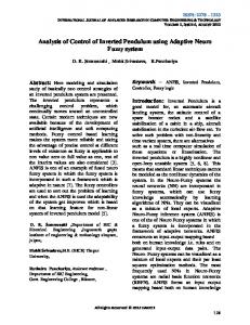
2 Mathematical model The inverted pendulum considered in this paper is given in Figure 1. A cart equipped with a motor provides horizontal motion, while cart position x, and joint angle θ, measurements can be taken via a quadrature encoder.
m
y
θ L
F
M
x
Figure 1: Inverted pendulum system
49
Issue 2, Volume 10, February 2011
WSEAS TRANSACTIONS on CIRCUITS and SYSTEMS
Valeri Mladenov
The velocities and accelerations in these directions can be calculated from
The pendulum’s mass “m” is assumed to be equally distributed on its body, so its center of gravity is at its middle of its length at “ l = L 2 ”. No damping or other kind of friction has been considered when deriving the model. The parameters of the model that are used in the simulations are below in Table 1.
xɺ G = xɺ + lθɺ cos θ ɺxɺG = ɺxɺ + lθɺɺ cos θ − lθɺ 2 sin θ ɺxɺ = ɺxɺ + lθɺɺ cos θ − lθɺ 2 sin θ G
yɺ G = −lθɺ sin θ ɺyɺG = −lθɺɺsin θ − lθɺ 2 cos θ
Table 1: Table of parameters Parameters Mass of pendulum, m Mass of cart, M Length of bar, L Standard gravity, g Moment of inertia of bar w.r.t its COG
Values 0.1 [kg] 1 [kg] 1 [m] 9.81 [m/s2]
The force equilibrium for the pendulum in x and y directions can be given as
I = mL2 12 ≈ 0.0083
− mɺxɺG + H = 0 V − mg − mɺyɺG = 0
[kg*m2]
The system is underactuated since there are two degrees of freedom which are the pendulum angle and the cart position but only the cart is actuated by horizontal force acting on it. The equations of motion can either be derived by the Lagrangian method or by the free-body diagram method. Using the second one we consider the system can be divided into two separate free-body diagrams as shown in Figure 2. The coordinates of the center of gravity of the pendulum can be written as
The torque and force equilibrium for the pendulum are
− Iθɺɺ + V l sin θ − H l cosθ = 0 F − M ɺxɺ − H = 0 Combining the above equations we obtain
(
)
− Iθɺɺ + mg − mlθɺɺsin θ − mlθɺ2 cosθ l sin θ −
(
)
− mxɺɺ + mlθɺɺcosθ − mlθɺ2 sin θ l cosθ = 0
(I + ml )θɺɺ − mgl sin θ + mlɺxɺcosθ = 0
xG = x + l sin θ
2
(
)
F − M ɺxɺ − mɺxɺ + mlθɺɺ cos θ − mlθɺ 2 sin θ = 0
and
yG = l cosθ
(M + m ) ɺxɺ + mlθɺɺ cosθ − mlθɺ
M ɺxɺ
2
sin θ = F
I θɺɺ mɺxɺG
H F
V
mg
H
mɺyɺG
V Figure 2: Free body diagrams of cart and pendulum
By solving for ɺxɺ , and θɺɺ and introducing the state variables x1 = θ , x2 = θɺ , x3 = x , x4 = xɺ and u = F , the inverted pendulum system can be described in state space form
ISSN: 1109-2734
I + ml 2 ml cos θ
50
ml cos θ θɺɺ mgl sin θ = 2 M + m ɺxɺ F + mlθɺ sin θ
Issue 2, Volume 10, February 2011
WSEAS TRANSACTIONS on CIRCUITS and SYSTEMS
Valeri Mladenov
θɺɺ M + m −ml cos θ mgl sin θ 1 = 2 2 2 2 2 2 x ( I + ml ) ( M + m) − m l cos θ −ml cosθ I + ml F + mlθɺ sin θ ɺɺ 2 2 ɺ2 θɺɺ 1 ( M + m ) mgl sin θ − m l θ sin θ cos θ − ml cos θ ⋅ F = x ∆ (θ ) −m 2l 2 g sin θ cos θ + ( I + ml 2 ) mlθɺ 2 sin θ + ( I + ml 2 ) ⋅ F ɺɺ
where
(
)
∆ (θ ) = I + ml 2 (M + m) − m 2 l 2 cos 2 θ xɺ1 = x2 xɺ2 =
( M + m ) mgl sin x1 − m2l 2 x22 sin x1 cos x1 − ml cos x1 ⋅ u ( I + ml 2 ) ( M + m ) − m2l 2 cos2 x1
xɺ3 = x4
(1)
−m l g sin x1 cos x1 + ( I + ml ) mlx sin x1 + ( I + ml ) ⋅ u 2 2
xɺ4 =
2
2 2
( I + ml ) ( M + m ) − m l 2
2 2
equilibrium point, i.e. x eq = [π
equilibrium point, i.e. x eq = [ 0 0 x 0] , where x is T
The
state
space
0 x 0] ).
equations
T
linearized
around
θ θɺ x xɺ = [ 0 0 0 0] are
any point on the track where the cart moves) and when
T
T
1 0 0 0 − ml x δ 1 0 0 0 δ x ( I + ml 2 ) ( M + m ) − m 2 l 2 2 + u 0 0 0 1 δ x3 2 I + ml δ x4 0 0 0 ( I + ml 2 ) ( M + m ) − m 2 l 2
The eigenvalues of this linearized system with the parameter values given in Table 1, are λ1 ≈ −3.9739 , λ2 ≈ 3.9739 , λ3 = 0 , λ4 = 0 . Since one of the eigenvalues λ2 ≈ 3.9739 is positive (i.e. in the right half plane), the upright equilibrium point is unstable. The objective of the control problem is to swing up the pendulum from its pending position or from another state to the upright position and balance it in that condition by using supervised learning. The control problem has two parts mainly, swinging up and balancing the inverted pendulum. For swing up control energy based methods (i.e. regulating the mechanical energy of the pendulum) [1], [2] and for balancing control linear control methods (i.e. PD, PID, state feedback, LQR, etc.) are common among classical techniques. Artificial neural networks, fuzzy logic algorithms and reinforcement learning [3], [4], [5] are
ISSN: 1109-2734
cos2 x1
the pendulum is at its upright position (unstable
The equilibrium points of the inverted pendulum are when the pendulum is at its pending position (stable
0 ( M + m ) mgl δ xɺ1 δ xɺ ( I + ml 2 ) ( M + m ) − m 2 l 2 2 = δ xɺ3 0 −m 2l 2 g δ xɺ4 ( I + ml 2 ) ( M + m ) − m 2 l 2
2
(2)
used widespreadly in machine learning based approaches both for swing up and balancing control phases.
3 The control problem A simple controller in order to swing up the pendulum from its pendant position can be developed by means of physical reasoning. A constant force can be applied to the cart according to the direction of the angular velocity of the pendulum so that the pendulum would swing till the vicinity of the upright position. The balancing controller is a stabilizing linear controller which can either be a PD, PID or be designed by pole placement techniques (e.g. Ackermann) or by LQR. Here a PD controller is selected. The switching from the swinging controller to the linear controller is done when the pendulum angle is between θ = [ 0°, 20°] , or when
51
Issue 2, Volume 10, February 2011
WSEAS TRANSACTIONS on CIRCUITS and SYSTEMS
Valeri Mladenov
θ = [340°, 360°] . This controller can formally be presented as below
(
)
ɺ K 1 (0 − θ ) + K 2 0 − θ , u = u θ , θɺ = K 1 (2π − θ ) + K 2 0 − θɺ , F0 sgn θɺ ,
( )
( ()
if
)
if
where F0 = 2 N, K1 = −40 , K1 = −10 . The closed loop poles obtained with these gains are -10.6026, 4.0315, 0, and 0. The results of the simulations performed with this controller with the initial conditions
0≤ θ ≤
π
9 17π ≤ θ ≤ 2π 9 else
(3)
x0 = [π 0 0 0] , without any kind of sensor noise or actuator disturbance are given in Figure 3. T
Simulation results with controller for infinite track length for x0 = [π 0 0 0] pendulum angular velocity [rad/s]
7 pendulum angle [rad]
6 5 4 3 2 1 5
10 time [sec]
15
5
0
-5
-10
20
4
1
2
0.5 cart velocity [m/s]
cart position [m]
0 0
10
0 -2 -4 -6 -8
0
5
10 time [sec]
15
20
0
5
10 time [sec]
15
20
0 -0.5 -1 -1.5
0
5
10 time [sec]
15
-2
20
2.5
Force acting on the cart [N]
2 1.5 1 0.5 0 -0.5 -1 -1.5 -2 -2.5
0
2
4
6
8
10 time [sec]
12
14
16
18
20
Figure 3: Simulation results with controller for infinite track length for x0 = [π 0 0 0] T
It can be observed from the Figure 3 that the pendulum has been stabilized in the upright position, whereas the cart continues its travel with a constant velocity.
cart’s travel limited since no cart position (or velocity) feedback is used. However with this teacher controller selection, it would be easier to visualize and thus to compare the input/output mappings of the teacher and the neural network. The input-output map (also called policy) of this nonlinear controller is given in Figure 4. Here the horizontal axis represents the pendulum angles and vertical axis represents the pendulum angular velocities, and colours represents the actuator forces corresponding to the pendulum angles and angular velocities. From the teacher, sensor values (i.e. pendulum angle and angular velocity) and actuator values (i.e. input force acting on the cart) can be
4 Neural network controllers The swing-up controller is developed by means of physical reasoning, which is related to applying a constant force according to the direction of the angular velocity of the pendulum. The teacher controller that is used here has only two inputs (i.e. pendulum angle and angular velocity), so it won’t be possible to keep the
ISSN: 1109-2734
52
Issue 2, Volume 10, February 2011
WSEAS TRANSACTIONS on CIRCUITS and SYSTEMS
Valeri Mladenov
The design can be separated into two phases; the teaching and the execution phases. The teaching phase for each demonstration can be presented graphically as it is shown in Figure 5a. There is sensor noise present in the simulations which is selected as normally distributed random numbers with different initial seeds for each demonstration. Also bandlimited white noise is added at the output of the controller to represent the different choices that a human demonstrator can make in the teaching phase, in order to make the demonstrations less consistent, and therefore a more realistic representation of human behavior.
recorded. The simulations are performed by using Matlab/Simulink and Neural Networks Toolbox.
Figure 4: Input-output map of the teacher controller
The simulations contain two phases, the demonstration and the execution phases. In both phases the simulations are performed by using a fixed step solver (ode5, Dormand-Prince) with a fixed step size of 0.1 sec.
Figure 5b: Execution phase for supervised learning
When the teaching phase is finished, the neural network is generated in order to be added to the model using Matlab’s gensim command. After that the execution phase shown in Figure 5b, starts with the nonlinear controller replaced with the neural network, and the actuator disturbance is removed. The Simulink model is shown in Figure 5c.
Figure 5a: Teaching phase for supervised learning
Figure 5c: Simulation scheme for execution phase
During the teaching phase, five examples (or demonstrations) are used, the variance of the normally distributed random numbers for sensor noise in each
a sampling time of 1 sec, which is close to the free swinging period of the pendulum. This means that the demonstrator can make an inconsistent action every second with a standard deviation of σ = 0.1 ≈ 0.316 N . Each demonstration starts from the pending initial position, x0 = [π 0 0 0] , and lasts 15 seconds. The pendulum angles for these 5 demonstrations are given in
demonstration is selected as σ 2 = ( π 180 ) rad 2 , which 2
corresponds to a standard deviation of 1° . The actuator disturbance, representing the different actions of the demonstrator has a noise power level of σ 2 = 0.1 N 2 and
ISSN: 1109-2734
53
Issue 2, Volume 10, February 2011
WSEAS TRANSACTIONS on CIRCUITS and SYSTEMS
Valeri Mladenov
trial-and-error according to the success of the network in the testing phase. The activation function that is used in the hidden layer is tan-sigmoid, whereas a linear activation function is used in the output layer. The network has been trained using a Levenberg-Marquardt backpropagation (i.e. trainlm training algorithm from Matlab) with a constant learning rate of 0.001. The weights are updated for 500 epochs. The desired m.s.e. levels are selected as the variance of the actuator disturbances, since the neural network would start fitting the noise after that value. The performance (mean square error) obtained with this network is given in Figure 8. It can be observed that the m.s.e. has converged but the desired mse level has not been reached although the m.s.e. level at 500th epoch is close (approx. 0.165) to the desired one (0.1). The plant input data (i.e. the target for the neural network), and its approximation obtained by the neural network at the end of the training session which is related to these examples are presented in Figure 9.
Figure 6.
Figure 6: Pendulum angles obtained from demonstrations
It can be observed from Figure 6 that in all demonstrations the pendulum is stabilized in the upright position. The input output (I/O) map of the teacher controller with the demonstrated trajectories in the θ , θɺ portion of the state space on top of it, is given in Figure 7. This figure can give a rough idea about which parts of the input-output space was visited during demonstrations.
5 Simulation results In this chapter we present the results obtained by using the training data given in the last chapter.
5.1 Training of the Neural Networks Figure 8: Training results with MLFF NN
5.1.1 Multilayer Feedforward Neural Network The MLFF NN which was selected in order to approximate the behaviour of the teacher (controller) has two inputs (pendulum angle and angular velocity) and a single hidden layer with 25 hidden neurons in it.
The green plot is obtained by using Matlab’s sim command in order to observe how well the neural network will fit the desired output with the pendulum angles and angular velocities from the demonstrations.
Figure 9: Actuator forces from demonstrations and MLFF NN approximation
Figure 7: θ , θɺ trajectories on top of I/O map
A closer look might be taken to the approximation of the 3rd demonstration in Figure 9 and it can be observed
The number of hidden layer neurons are selected by
ISSN: 1109-2734
54
Issue 2, Volume 10, February 2011
WSEAS TRANSACTIONS on CIRCUITS and SYSTEMS
Valeri Mladenov
The plant input data (i.e. the target for the neural network), and its approximation obtained by the neural network at the end of the training session which is related to these examples can be presented below in Figure 12. The green plot is obtained by using Matlab’s sim command in order to observe how well the neural network will fit the desired output with the pendulum angles and angular velocities from the demonstrations.
from Figure 10 that the neural network has made a good approximation.
Figure 10: Actuator forces from 3rd demonstration and MLFF NN approximation
5.1.2 Radial Basis Function Network The RBFN which was selected in order to approximate the behavior of the teacher (controller) has two inputs (pendulum angle and angular velocity). The centers of the gaussian functions are selected in a supervised manner. The training starts initially with no gaussian functions in the hidden layer, then gaussian functions are added incrementally such that the error between the target and network’s output becomes smaller. The spread (width of the gaussian functions) parameter is selected equal to 1, by trial-and-error according to the success of the network in the testing phase. The number of gaussian functions that are used in the hidden layer are 103. The desired m.s.e. levels are selected as the variance of the actuator disturbances, since the neural network would start fitting the noise after that value. The performance (mean square error) obtained with this network is given in Figure 11. It can be observed that the mse has converged but the desired mse level has not been reached although the m.s.e. level at the end of training is close (approx. 0.272) to the desired one. The training has stopped automatically after the radial basis neurons started overlapping.
Figure 12: Actuator forces from demonstrations and RBFN approximation
A closer look might be taken to the approximation of the 3rd demonstration in Figure 12 and it can be observed from Figure 13 that the neural network has made a fair approximation.
5.2 Testing of the Neural Networks The neural networks that are trained from the demonstration data are tested in two ways. First a data set that was not encountered during the training phase will be used.
Figure 13: Actuator forces from 3rd demonstration and RBFN approximation
This will be performed by simulating the inverted pendulum with initial pendulum angles incremented by π 180 (i.e. 1° ) between θ 0 = [ 0, 2π ] . The duration of the simulations in the execution phase is
Figure 11: Training results with RBFN
ISSN: 1109-2734
55
Issue 2, Volume 10, February 2011
WSEAS TRANSACTIONS on CIRCUITS and SYSTEMS
Valeri Mladenov
taken as 30 seconds. Secondly, the input-output maps of the neural networks will be compared in order to be able to determine how well the network has learned and generalized the control policy of the teacher. This will also help assessing the extrapolation capabilities of the designed networks. 5.2.1 Multilayer Feedforward Neural Network The pendulum angles for several initial pendulum angles from simulations in the execution phase are below in Figure 14. The MLFF NN managed to swing up and stabilize the pendulum in 361 out of 361 initial angles which corresponds to a success rate of 100 %.
Figure 15: Input-output map of MLFF NN
Initial pendulum angle, θ0 = 0.2536
Initial pendulum angle, θ0 = 3.1643 6 Pendulum angle [rad]
Pendulum angle [rad]
0.3 0.2 0.1 0 -0.1 -0.2 0
5 4 3 2 1 0
5
10
15 time [sec]
20
25
-1
30
0
5
Initial pendulum angle, θ0 = 4.0315
20
25
30
25
30
6.4
6
Pendulum angle [rad]
Pendulum angle [rad]
15 time [sec]
Initial pendulum angle, θ0 = 5.9828
7
5 4 3 2 1 0 0
10
5
10
15 time [sec]
20
25
6.3 6.2 6.1 6 5.9
30
0
5
10
15 time [sec]
20
Figure 14: Several pendulum angle plots from execution phase
The input output map of the neural controller can be given as follows in Figure 15. It can be observed from Figure 15 that the controller has learned most of the swinging region that is demonstrated to it, and it has made generalization errors in some regions marked with circles. The linear control region on the right and the angle to switch from swinging control to linear control has been learned better compared to the one on the left. This might be due to insufficiency of demonstrated data in those regions.
from simulations in the execution phase are below in Figure 16. The RBFN managed to swing up and stabilize the pendulum in 360 out of 361 initial angles which corresponds to a success rate of 99.7 %. The input output map of the neural controller can be given as follows in Figure 17. The circles at the corners of the plot have nearly zero output, this would most probably be related to the fact that radial basis functions give nearly zero output outside their input range. The network has learned to separate the swing up region into two, even though there are some generalization errors.
5.2.2 Radial Basis Function Network The pendulum angles for several initial pendulum angles
ISSN: 1109-2734
56
Issue 2, Volume 10, February 2011
WSEAS TRANSACTIONS on CIRCUITS and SYSTEMS
Valeri Mladenov
Initial pendulum angle, θ0 = 0.091414
Initial pendulum angle, θ0 = 3.1475 6 Pendulum angle [rad]
Pendulum angle [rad]
0.15 0.1 0.05 0 -0.05 -0.1
5 4 3 2 1 0
0
5
10 time [sec]
15
-1
20
0
Initial pendulum angle, θ0 = 4.0613
15
20
6.4
5
Pendulum angle [rad]
Pendulum angle [rad]
10 time [sec]
Initial pendulum angle, θ0 = 6.1998
6
4 3 2 1 0 -1 0
5
5
10 time [sec]
15
6.35 6.3 6.25 6.2 6.15
20
0
5
10 time [sec]
15
20
Figure 16: Several pendulum angle plots from execution phase
6 Conclusion The supervised learning method of the Neural Networks controllers consists of two phases, demonstration and execution. In the demonstration phase necessary data is collected from the supervisor in order to design a neural network. The objective of the neural network is to imitate the control law of the teacher. In the execution phase the neural controller is tested by replacing the teacher. The Neural Network control strategy is tested by using a supervisor, with a control policy that ignores the finite track length of the cart. By this way, it is easier to understand what the neural controller that is used to imitate the teacher does, by comparing the input/output (state-action) mappings using 2D colour plots. The policy of a demonstrator (i.e. designed controller in this case) is not a function that can be directly measured by giving inputs and measuring outputs, so learning the complete I/O map and making a perfect generalization would not be possible. The complexity of the function that would be approximated is also important since the function may include both continuous and discontinuous components (such as switches between different control laws). All of the designed neural networks controllers (MLFF NN and RBFN) are able to learn the demonstrated behaviour which was swinging up and balancing the inverted pendulum in the upright position starting from different initial angles. The MLFF NN did a better job by means of generalization and obtaining lowest training error compared to the RBFN.
Figure 17: Input-output map of RBFN
5.3 Comparison of the Results The first thing that can be noticed from the results is that the interpolation capabilities the networks are quite close to each other. This can be observed from the fact that all networks can swing up and balance the inverted pendulum starting from any initial pendulum angle between θ 0 = [ 0, 2π ] . It can further be examined from the input-output maps, since the parts of the input-output space which were related to the demonstrated data was learned quite well by all networks. The least training error was obtained by using a MLFF NN. The extrapolation capabilities of MLFF NN are better compared to RBFN. The RBFN also contains more hidden neurons (gaussian functions) compared MLFF NN. A better generalization is also possible for MLFF NN by taking more and different training data.
ISSN: 1109-2734
57
Issue 2, Volume 10, February 2011
WSEAS TRANSACTIONS on CIRCUITS and SYSTEMS
Valeri Mladenov
References: [1] M. Bugeja, “Nonlinear Swing-Up and Stabilizing Control of an Inverted Pendulum System”, Proc. of EUROCON 2003 Computer as a Tool, Ljubljana, Slovenia, vol.2, 437- 441, 2003. [2] K. Yoshida, “Swing-up control of an inverted pendulum by energy based methods”, Proceedings of the American Control Conference, pp. 40454047, 1999. [3] Darío Maravall, Changjiu Zhou, Javier Alonso, “Hybrid Fuzzy Control of the Inverted Pendulum
ISSN: 1109-2734
via Vertical Forces”, International Journal of Intelligent Systems, vol. 20, pp. 195–211, 2005. [4] The Reinforcement Learning Toolbox, Reinforcement Learning for Optimal Control Tasks, G. Neumann, May 2005. http://www.igi.tugraz.at/riltoolbox/thesis/DiplomArbeit.pdf [5] H. Miyamoto, J. Morimoto, K. Doya, M. Kawato, “Reinforcement learning with via-point representation”, Neural Networks, vol. 17, pp. 299– 305, 2004.
58
Issue 2, Volume 10, February 2011