Modified Census Transform, Total Variation. 1 Introduction. Nowadays, image processing and computer vision are widely used in the automa- tion industry.
Application of Optical Flow in Automation Mahmoud A. Mohamed and B¨arbel Mertsching GET Lab, University of Paderborn, 33098 Paderborn, Germany {mahmoud, mertsching}@get.upb.de http://getwww.upb.de
Abstract. The optical flow allows the estimation of the apparent motion of objects. An adequate algorithm yields information about the velocities and the directions of objects which can be used for industrial automation purposes. This paper discusses a method based on the total variation approach with the usage of the modified census transform [1] for a pick and place scenario with a robot in a production line. After its implementation the approach is evaluated with real data to check its efficiency. It can be shown that it produces accurate optical flow results. Keywords: Motion Estimation, Optical Flow, Industry Automation, Modified Census Transform, Total Variation
1
Introduction
Nowadays, image processing and computer vision are widely used in the automation industry. One of the most challenging tasks is the detection and estimation of motion of objects. This can be used in various applications such as driver assistance systems and automation. In the field of grasping, the robot should be able to detect and grasp the object during the object’s movement. Fig. 1 shows two frames in an automation process: In a pick and place scenario, a robot in a production line should pick an object from a conveyor belt1 . The robot, in this case, can grasp static objects easily, while it has difficulties grasping moving objects because the robot does not have enough information about the current location and the relative velocities of objects. It can be shown that an active vision system can easily solve this problem. A motion estimation algorithm provides information about the velocity and the direction of the object and helps the robot to correctly locate the object. Results are shown in fig. 1. The color coding proposed in [2] has been used to represent the optical flow. There are two basic approaches for the estimation of optical flow: The first one was developed by K. P. Horn and B. G. Schunck [3] while the second originates from B. D. Lucas and T. Kanade [4]. Lucas and Kanade used a local method assuming that small regions of pixels have the same flow while Horn’s 1
The images were taken at the Lemgo model factory (http://www.hsowl.de/init/research/lemgoer-modellfabrik.html) – the support by InIT is greatly acknowledged.
2
Mahmoud A. Mohamed and B¨ arbel Mertsching
Fig. 1. Top: Two consecutive frames of a moving object taken from the Lemgo model factory. Bottom: Right: Representation of optical flow using arrows; left: color coded optical flow.
and Schunck’s model is based on global optimization proposing a variation approach to find the optical flow’s values. To enhance the estimation accuracy of large displacements, A. Bruhn et al. [5] proposed a new variation approach named CLG combining local and global methods. M. Drulea and S. Nedevschi [6] introduced a variation model with a parallel numerical scheme. Here, a CLG with the total variation L1-norm instead of the L2-norm is used. Furthermore, they applied a bilateral filter on the data term and used a diffusion filter to limit the propagation of the optical flow among adjacent pixels. The authors of this paper could show recently [1] that a combination of the total variation with the modified census transform integrated with a weighted median filter produces accurate optical flow results. The goal of the work presented here is to produce accurate optical flow results based on a variation optical flow with a technique for recovering motion of small image details. Our approach is based on the L1 total variation minimization algorithm combined with the CLG approach. Furthermore, the correspondences from the modified census transform are used for recovering lost image details during the implementation of the coarse-to-fine levels. A weighted median filter is integrated to prevent the propagation among pixels in different regions. The overall algorithm is shown in fig. 2. The results of this algorithm after integrating
Application of Optical Flow in Automation
3
Fig. 2. The overall algorithm using two frames of the Army sequences of the Middlebury database [2].
it to an active vision system will be sent to the robot to enable it to locate and grasp objects. The paper is organized as follows: Section 2 discusses the recovering of image details using the modified census transform while the overall motion estimation approach will be presented in section 3. The use of real data to evaluate the performance of the proposed algorithm is discussed in section 4 followed by the conclusion in section 5.
2
Modified Census Transform
Relying on the relative ordering of local intensity values instead of the intensity values themselves the census transform is a non-parametric transform which is very robust with respect to outliers. Its main idea is the retrieval of a set of promising image-to-image correspondence hypotheses [7]. Applying the census operator to two consecutive images results in binary signature vectors of a fixed length [8] for each image containing information about all the adjacent pixels. The transform produces a high texture density in areas with high structural information. Stein [7] defines the census transform as a transform which maps a local neighborhood surrounding a pixel P to a ternary string representing the set of neighboring pixels. Each census vector ξ(P, P 0 ) is defined as: P − P0 > ε 0 0 ξ(P, P ) = 1 (1) |P − P 0 | ≤ ε 0 2 P −P >ε where ε is a threshold. In this work, we have used the modified census transform (M CT ), originally proposed in [9] for face recognition algorithms, to com-
4
Mahmoud A. Mohamed and B¨ arbel Mertsching
pare the intensity of a pixel with the average intensity in a block instead of that of the center pixel. Although the census transform solves the correspondence problem between two images in a very efficient way, the result has major drawbacks. First, it produces a sub-pixel output. Second, the outliers of the matching correspondences cause strong disturbances in the motion calculation at image discontinuities. Our goal was to combine the sparse matching correspondences with a variation model which could be used as an initial value for each new level during a coarse to fine optimization process.
3
The Motion Estimation Model
In this section, the proposed approach is represented in more detail. We integrated the CLG [5] algorithm with the L1 total variation algorithm in the energy function to be: � �i Xh � 2 2 ψ wT Jρ (∇3 f ) w + λ1 (ψ (∇u) + ψ (∇v)) + λ2 (u − u ˆ) + (v − vˆ) E= (2) √ where ψ(x2 ) = x2 + ε2 and ε = 0.01 to prevent the division by zero. w = (ˆ u, vˆ, 1)T where u ˆ and vˆ are auxiliary optical flow variables. f is the original image I(x, y) convolved with a Gaussian Kσ (x, y) with standard deviation σ, while ∇3 f = (fx , fy , ft )T . Jρ is the Gaussian Kρ (x, y) with a standard deviation ρ and Jρ (∇3 f ) = Kρ ∗ (∇3 f ∇3 f T ). The last term λ2 ((u − u ˆ)2 + (v − vˆ)2 ) is used to enforce u ˆ and u to be equal. λ1 and λ2 are regularization parameters. The function (2) can be decomposed as in [10] into three parts: � �i Xh � 2 2 ED = ψ wT Jp (∇f ) w + λ2 (u − u ˆ) + (v − vˆ) (3) i 2 λ2 (u − u ˆ) + λ1 ψ (∇u) i Xh 2 Ev = λ2 (v − vˆ) + λ1 ψ (∇v)
Eu =
Xh
(4) (5)
where u ,v are constants and ED has two unknowns u ˆ, vˆ. The optimal solution for u ˆ,ˆ v does not depend on spatial derivatives of u ˆ and vˆ and is calculated point-wise by using the Euler-Lagrange equation, then optimized by using a least square minimization. Similarly, Eu and Ev have two unknowns u and v, while u ˆ and vˆ are constants. We have used the numerical scheme in [6] to solve Eu and Ev . The Euler-Lagrange equation for Eu is: � � (∇u) (u − u ˆ) − λ div =0 (6) ψ(∇u) let Pu = ∇u/ψ(∇u), then we have u = λ div(Pu ) + u ˆ,
(7)
Application of Optical Flow in Automation
5
which can be solved using a fixed-point iteration scheme as in [6] Pun+1 =
Pun + τ ∇(div(Pun ) + λuˆ ) 1 + τ ||∇(div(Pun ) + λuˆ )||
(8)
where τ ≤ 1/8 is the time step.The same can be applied to get Pv . Equation (2) is isotropic and propagates the flow in all directions regardless of local properties. In order to enhance the propagation, the weighted median filter was used to solve the isotropic propagation problem as introduced in [11, 12]. We applied the algorithm in [13], but integrated the spatio-temporal image segmentation approach introduced in [14] to calculate the weighted function: X (9) ui,j − ui0 ,j 0 | u ˆi,j = min ωi,j,i0 ,j 0 |ˆ 0
0
where (i , j ) ∈ Ni,j and Ni,j is the N × N local window, and ω ∈ [0, 1]. The approach in [14] segments the image into three different regions, moving texture, moving homogeneous and stationary regions based on the spatial and temporal image derivatives. SN R 6 τ, | cos(δ)| ' 1, | cos(β)| ' 0 M oving − T exture; I(x, y, t) ∈ M oving − Homogenous; SN R > τ, || cos(δ) ' 1 Stationary; otherwise (10) where SN R is the signal-to-noise ratio of the gradient magnitudes and δ is the angle between the spatio-temporal gradient (Ix , Iy , It )T and a unit vector (0, 0, 1)T . β is another angle which | cos(β)| is close to one when the image gradient is very small. If a seed pixel belongs to a textured region while a neighboring pixels belong to a homogeneous region, then the propagation should not be affected by such pixels and thus ω = 0. Similarly, if both pixels belong to the same type of region (homogeneous or textured) but the states are different, i.e. one is a moving region and the other is a static region, then ω = 0; otherwise ω = 1. We have used the warping technique as in [15] to improve the coarse-to-fine module. At each level of coarse-to-fine scheme, the solution of equations (7) and (8) are calculated iteratively. The initial values of u, v are propagated from each coarser level into the finer one. The matching correspondences are calculated giving a set of hypothesis points. These points are used to refine the propagated values from the coarser level. At this stage, we have two initial sources of data: (a) matching correspondences which neglect regularity and (b) propagated values from the coarser level which neglects image details. Our proposed algorithm integrates both sources of information to the calculation of the initial values. In case that there is no matching correspondence, only the propagated value from the coarser level is considered. Otherwise, a fusing function is used to validate the motion vector values based on the neighborhood pixels information. This decision is done by comparing the mean value of the vector lengths d¯p of the propagated (N × N ) window values and the vector length dc of the matching correspondences. dc is assumed
6
Mahmoud A. Mohamed and B¨ arbel Mertsching
to be an outlier in case that the difference between dc and d¯p is larger than a threshold and then only the propagated value is considered. On the other hand, if the propagated value is similar to the neighbor pixels while its location is not homogeneous, then it is probable that motion information was lost in the interpolation process. In such a case, we consider only the matching correspondences. The initial values for the first coarse level are set to the values of matching correspondences instead of zeros in other approaches.
4
Experimental Results
The optical flow algorithm was tested using real image sequences from the Lemgo model factory. The first image sequence is shown in fig. 3. In this sequence, the camera was on an horizontal position on the top of moving object. As we can see in fig. 3 the algorithm correctly estimated the motion of the object. The object moved from right to left, which is represented by the blue color in the color representation. The second sequence is shown in fig. 4. In this sequence, the camera was portable and facing many moving objects in the scene. The optical flow algorithm succeeded to detect and estimate the motion of the objects. The objects were moving from left to right and the motion is display by the red color. The global color which appears in this sequence represents the global motion due to the camera motion which is also called ego-motion. The parameters used in these experiments are as follow: The outer fixed point iteration value was 8 and the inner fixed point iteration was 2 while λ = 8. The census transform used a window of 5 × 5 to construct the signatures within a search window size of 50 pixels; the maximum frequency occurrence value was 1 and the vector size was 20 digits, while the coarse-to-fine factor was 0.5. The implementation of this approach was done using C++ and the opencv library on a PC with an Intel(R) Core(TM)2 Duo CPU with 3.33 GHZ. The images had 1280 × 720 pixels and the execution time was about 28 sec for 2 frames. The implementation does not work in real time, but this can be achieved easily using a parallel implementation on a GPU.
5
Conclusion
In this paper, a combined L1 total variation and CLG optical flow approach integrating a module for recovering motion of small image details was used to obtain accurate optical flow results which contain important information for a robot to detect, localize and grasp the moving objects. A modified census transform algorithm was used to improve the recovering module while a weighted median filter was applied to prevent pixel propagation among different regions. The proposed approach used the matching corresponding output of the modified census transform module as initial values for solving the variation minimization equation during the coarse-to-fine scheme to recover the lost motion of the small image details . In addition, the possible matching correspondences are limited by considering only strong matching in order to improve the overall computational
Application of Optical Flow in Automation
7
Fig. 3. Odd images sequence. Odd rows show the images while the even rows show the optical flow between each image and the next image in this sequences.
time. Moreover, the weighted median filter was used to prevent the propagation among different regions with different motion.
References 1. Mohamed, M.A., Mertsching, B.: TV-L1 optical flow estimation with image details recovering based on the modified census transform. In: Int. Symposium on Visual Computing (ISVC). (2012) 2. Baker, S., Scharstein, D., Lewis, J., Roth, S., Black, M., Szeliski, R.: A database and evaluation methodology for optical flow. In: Int. Journal of Computer Vision. Volume 92., Springer (2011) 1–31 3. Horn, B., Schunck, B.: Determining optical flow. In: Artificial intelligence. Volume 17., Elsevier (1981) 185–203 4. Lucas, B., Kanade, T.: An iterative image registration technique with an application to stereo vision. In: Proc. of DARPA Image Understanding Workshop. (1981) 121–130 5. Bruhn, A., Weickert, J., Schn¨ orr, C.: Lucas/Kanade meets Horn/Schunck: Combining local and global optic flow methods. In: Int. Journal of Computer Vision. Volume 61., Springer (2005) 211–231 6. Drulea, M., Nedevschi, S.: Total variation regularization of local-global optical flow. In: Proc. of Intelligent Transportation Systems (ITSC), IEEE (2011) 318–323 7. Stein, F.: Efficient computation of optical flow using the census transform. In: Proc. of DAGM, Springer (2004) 79–86
8
Mahmoud A. Mohamed and B¨ arbel Mertsching
Fig. 4. Odd rows show the images while the even rows show the optical flow between each image and the next image in this sequences.
8. Zabih, R., Woodfill, J.: Non-parametric local transforms for computing visual correspondence. In: Proc. of European Conference on Computer Vision (ECCV), Springer (1994) 151–158 9. Froba, B., Ernst, A.: Face detection with the modified census transform. In: Proc. of Automatic Face and Gesture Recognition, IEEE (2004) 91–96 10. Chambolle, A.: An algorithm for total variation minimization and applications. In: Journal of Mathematical Imaging and Vision. Volume 20., Springer (2004) 89–97 11. Buades, A., Coll, B., Morel, J.: A non-local algorithm for image denoising. In: Proc. of Computer Vision and Pattern Recognition (CVPR). Volume 2., IEEE (2005) 60–65 12. Gilboa, G., Osher, S.: Nonlocal operators with applications to image processing. In: Multiscale Model and Simulation. Volume 7. (2008) 1005–1028 13. Sun, D., Roth, S., Black, M.: Secrets of optical flow estimation and their principles. In: Proc. of Computer Vision and Pattern Recognition (CVPR), IEEE (2010) 2432– 2439 14. Rashwan, H., Puig, D., Garcia, M.: On improving the robustness of differential optical flow. In: Proc. of Int. Conference on Computer Vision Workshop (ICCV Workshop), IEEE (2011) 876–881 15. Brox, T., Bruhn, A., Papenberg, N., Weickert, J.: High accuracy optical flow estimation based on a theory for warping. In: Proc. of European Conference on Computer Vision (ECCV), Springer (2004) 25–36