Application of the PageRank algorithm for ranking locations of a production network. Bernd Scholz-Reiter1 (2), Fabian Wirth2, Sergey Dashkovskiy3,. Thomas ...
Application of the PageRank algorithm for ranking locations of a production network Bernd Scholz-Reiter1 (2), Fabian Wirth2, Sergey Dashkovskiy3, Thomas Makuschewitz1, Michael Kosmykov3, Michael Schönlein2 1 Planning and Control of Production Systems (PSPS), BIBA – Bremer Institut für Produktion und Logistik GmbH at the University of Bremen, Bremen, Germany 2 Institute of Mathematics, University of Würzburg, Würzburg, Germany 3 Centre of Industrial Mathematics, University of Bremen, Bremen, Germany
Abstract In order to investigate the dynamics of large-scale production networks it is essential to derive representative models of lower size. Against this background two questions occur: How to identify locations that might be neglected? How to identify locations that are highly important for the original network? In this paper it will be presented an approach that allows determining the relative importance of locations within one production network. The approach is based on an adaptation of the PageRank algorithm used by Google. The algorithm considers both the network structure and the intensity of the material flows. Furthermore the approach is able to take changes of material flows over time into account. The computational analysis suggests that the results are promising for effectively identifying the most representative locations in production networks. Keywords: Decision making, Structural analysis, Ranking
1 INTRODUCTION Modern production networks have become very large and global [1]. Planning and control of production and logistics processes in such networks is more and more determined by an increasing complexity of structure and dynamics. The dynamical behaviour of these networks is characterised not only by local and interacting dynamics of specific locations but also by changes in the structure of the network. For example experienced partners might leave and new partners join the network. In order to analyse and control such complex and dynamic networks methods and tools are required, which take the stability and robustness of the network into account [2]. For the investigation of large-scale production networks it is essential to derive representative models of lower size. A model of lower size that exhibits almost the same dynamics as the original network would facilitate the analysis of the network and the associate processes. In regard to the dynamics of the network not all locations have the same influence on the networks behaviour. Locations that are highly important should have a large influence on the behaviour of the network. On the other hand locations, which are less important, have a small influence and might be omitted in a model of reduced size. This raises two questions: How to identify locations that might be neglected? How to identify locations that are highly important for the analysis of the network? In order to determine the relative importance of locations for the network the structure of the production network itself is a valuable source of information. An algorithm that makes use of this information is the PageRank algorithm [3], which has been a core component of the Google search engine in its early days. The PageRank algorithm can be used to determine the rank of a given location within a production network by taking its links to other locations pointing to it and the ranks of these referring locations into account. In comparison to the Internet a production network is not only characterised by a similar linked structure but also by the material flows between locations. Hence, the original algorithm has to be adapted to this specific setting. The
proposed algorithm considers both the networks’ structure and the intensity of the material flows between locations. Furthermore the approach is able to take changes of the material flows within the production network over time into account. Hence, a dynamic ranking is obtained. The paper is organised as follows. In section 2.1 an adaptation of the original PageRank algorithm for production networks is presented. This concept is used as starting point for the modifications of the algorithm in order to cope with the capabilities described above. These modification steps are introduced in section 2.2 and 2.3. Section 3 presents a simple production network, which will be used to evaluate the obtained ranking by the adapted PageRank algorithm. An optimisation model for the generation of material flows for the test case is briefly introduced in section 4. The computational analysis of section 5 aims to provide an insight into the dependence of the adapted ranking scheme on control parameters and the observed material flows. Section 6 concludes the paper and makes some suggestions for future research. 2
RANKING OF LOCATIONS WITHIN PRODUCTION NETWORKS
2.1 Application of PageRank A global production network is usually shaped by a large number of suppliers, OEM locations, warehouses and retailers. As soon as the structure of the network, starting from an n-tier supplier and ending at a retailer, is not arranged in a linear way, not all locations have the same importance for the whole network. The reason therefore is a non-linear structure of the network and a different intensity of the material flows that connect the locations. A supplier that produces twice as much as another supplier of the same pre-product is for instance more important for the network. Despite this obvious correlation interdependences between locations of different kinds have to be considered as well. Hence, a major retailer might give more importance to a set of smaller suppliers that deliver mainly pre-products for the products that are sold by the retailer.
In order to identify the importance of locations, the structure of the network itself is a valuable source of information. The Google PageRank algorithm [3] makes use of this information and was used originally to rank the importance of websites in the internet. The rank (importance) of a location i within a production network depends on how many locations order material from this location. The more important locations order material from a given location the more important it is. Thus the location gets a high rank. Locations share their rank equally between their suppliers. If a location supplies only a few other low ranked locations it gets as well a low rank. For a given network with n locations the rank of a certain
network to the retailers can contribute their rank to the retailers. Thus, a retailer that can initiate the production at many L-tier suppliers is more important for the network than a supplier compared to a supplier that is only linked to a small number of L-tier suppliers. In Figure 1 retailers five and six are linked to both 1st-tier suppliers and retailer seven only to the 1st-tier supplier 2. Hence, retailer seven should be less important for the production network.
location can be derived by Equation (1). The set I is contains all locations that are supplied by location i. Thus the rank NRi of location i is the sum of the fraction of rank that all locations j contribute and a small positive term. The contributed share of a certain location j depends on the rank NRj of location j and the number of suppliers Nj. In the case that a location has no suppliers it would act like a rank sink. In order to balance the system these locations share their rank equally to all other locations of the network. Therefore each location gets a small positive amount of rank from all other locations that is given by the second term of Equation (1).
NRi = α
NR j
∑N j ∈I is
j
+ (1 − α )
1 n
(i ∈ I )
(1)
The number of locations within the production network is n; 0≤α≤1, 1-α is treated as a probability that a location supplies material to locations with which it has no direct link (partnership). Furthermore α can be used to adjust the influence of the networks’ structure on the ranking. For example an α close to one would give almost all attention to the structure of the production network. In order to compute the ranks of the locations the production network will be treated like a directed graph. Figure 1 shows a small example of a production network that is organised in three levels. The original network consists of two 1st-tier suppliers, two OEM locations and three retailers, which are linked by material flows. For simplicity we assume that the placement of an order by a retailer initiates the production at the first production level L. In this case the 1st-tier suppliers. Starting from the 1sttier suppliers the orders are processed in downstream direction of the material flows within the production network until they are delivered to the retailers. This correlation between the placement of an order by a retailer and the start of the manufacturing process of the L-tier suppliers is illustrated by the dashed lines in Figure 1. The dashed lines represent the information flow between these specific locations. The additional links are treated like ‘physical’ links of the original production network and are incorporated into the adapted ranking scheme. By introducing the additional links the ranking obtains the capability to differentiate between different kinds of retailers. Since, the retailers do not have any customers within the original production network they would have been treated like rank sources and would have gained the same importance. The new links connect the rank sinks (L-tier suppliers) with the rank sources (retailers) of the original production network. Thus the retailers obtain their rank from the L-tier suppliers. By connecting the L-tier suppliers with the retailers the ability to satisfy the demand of a retailer by a L-tier supplier needs to be considered. Only L-tier suppliers that are linked within a sub-graph of the original production
Figure 1 The adjacency matrix A=(aij) of the graph describes the interconnected structure of the production network. The elements aij of this matrix are either one (location i supplies location j) or zero (locations i does not supply location j). For the production network of Figure 1 the adjacency matrix is given by the following matrix A of the graph:
⎛0 ⎜ ⎜0 ⎜0 ⎜ A = ⎜0 ⎜ ⎜1 ⎜1 ⎜⎜ ⎝0
0⎞ ⎟ 0⎟ 0 ⎟⎟ 1⎟ ⎟ 1 0 0 0 0 0⎟ 1 0 0 0 0 0⎟ ⎟ 1 0 0 0 0 0 ⎟⎠
0 0 0 0
1 1 0 0
0 1 0 0
0 0 1 0
0 0 1 0
(2)
The Power method [4] can be used to obtain an approximate numerical solution of Equation (1). For this purpose the adjacency matrix A needs to be transformed according to the following four steps. 1. Transpose AT = (aTij ) 2.
(3)
Normalization
⎛ ⎜ H = (H ij ) = ⎜ ⎜⎜ ⎝ 0 ⎛ 0 ⎜ 0 ⎜ 0 ⎜ 0 . 5 0 .5 ⎜ H =⎜ 0 1 ⎜ 0 0 ⎜ ⎜ 0 0 ⎜⎜ 0 0 ⎝
aTij
∑
n k =1
aTjk
⎞ ⎟ ⎟ ⎟⎟ ⎠
0 0 0 .5 0 .5 0 ⎞ ⎟ 0 0 0.333 0.333 0.333 ⎟ 0 0 0 0 0 ⎟⎟ 0 0 0 0 0 ⎟ ⎟ 1 0 0 0 0 ⎟ 1 0 0 0 0 ⎟ ⎟ 0 1 0 0 0 ⎟⎠
(4)
(5)
3.
material flows within a production network can be incorporated into the ranking.
Make the matrix stochastic
S=H+
ee T beT , E= , e = (1,K,1)T ∈ R n n n
⎧ n ⎪1, H ij = 0 ⎪ ⎪ j =1 bi = ⎨ ⎪ n H ij = 1 ⎪0, ⎪⎩ j =1
∑
(6)
∑
For the graph of Figure 1 the matrix it is already stochastic. 4.
Make the matrix primitive
G = αS + (1 − α )E
(7)
For the matrix A in Equation (2) we use α=0.85 and obtain: ⎛ 0.0214 ⎜ ⎜ 0.0214 ⎜ 0.5314 ⎜ G = ⎜ 0.0214 ⎜ ⎜ 0.0214 ⎜ 0.0214 ⎜⎜ ⎝ 0.0214
0.0214 0.0214 0.0214 0.7014 0.1914 0.0214 ⎞ ⎟ 0.0214 0.0214 0.0214 0.2481 0.0781 0.5881 ⎟ 0.3614 0.0214 0.0214 0.0214 0.0214 0.0214 ⎟ ⎟ (8) 0.8714 0.0214 0.0214 0.0214 0.0214 0.0214 ⎟ ⎟ 0.0214 0.8714 0.0214 0.0214 0.0214 0.0214 ⎟ 0.0214 0.8714 0.0214 0.0214 0.0214 0.0214 ⎟ ⎟ 0.0214 0.0214 0.8714 0.0214 0.0214 0.0214 ⎟⎠
Matrix G is primitive and irreducible [5]. The problem of finding a solution for Equation 1 is equivalent to the problem of finding unique eigenvector p of G that corresponds to the eigenvalue 1: pT G = pT
(9)
The vector p is the vector of ranks for the considered production network. The Power method allows finding approximately the eigenvector of a matrix that corresponds to a maximal absolute eigenvalue (spectral radius). The kth step of the iteration process of the power method is: p ( k +1)T = p ( k )T G
(10)
The Perron-Frobenius theorem for irreducible, nonnegative matrices guarantees the existence of the unique rank vector p that is the eigenvector of G corresponding to the spectral radius that is equal to 1. Primitiveness of matrix G guarantees convergence of the Power method ([4]). The computational time of the power method is even relatively small for large matrices. Thus this approach can be easily extended to large-scale production networks. The rank vector for the network of Figure 1 is: p = (0.126; 0.200; 0.245; 0.088; 0.132; 0.132; 0.078) In particular location three is the most important location of the network. The second highest rank has location two. Another characteristic result is given by the ranks of locations five and six. They have the same rank, because they obtain the same share of rank from the locations one and two. In the real world these two locations might have a different importance for the network. The reason might be a different volume of orders that is placed by these retailers. Hence, the material flow within a production network is a valuable source of information as well. In the next section it will be discussed how the intensity of
2.2 Incorporation of material flows So far only the structure of the production network has been taken into account to derive the ranks of the locations. Another valuable source of information is the intensity of material flows within a production network. Since the flows are different between the locations they also reflect the relations between the various locations of the network. A supplier which satisfies a large fraction of the demand for a certain product of a location is for instance more important than a supplier that only contributes a small share. These data can be taken into account to adjust the rank distribution of a certain location within the set of its suppliers. In this case the rank of location i depends on the share of ordered material that it delivers to other locations. The larger this share of delivered material to high ranked locations is the higher gets the rank the location. For this purpose the observed intensity of material flows between the locations will be used to weight the links of the graph. Thus, the weights represent the total amount of material shipped between two locations for a certain period of time. These weights are used to set up the weighted adjacency matrix A=(aij) of the graph. Instead of zeros and ones the elements aij represent the total amount of material shipped from location i to location j. Since, the introduced links between retailers and L-tier suppliers represent information flow they cannot be weighted at this stage with an observed material flow. Furthermore it is in general time-consuming to analyse the quantity of material, which was provided by a certain L-tier supplier in order to satisfy the demand of a certain retailer. Therefore the rank of a certain L-tier supplier is distributed among the retailers as follows: The rank will be distributed between the retailers that are linked within a sub-graph of the original production network to the L-tier supplier. Each retailer obtains a share of the L-tier suppliers’ rank according to the ratio of his demand compared to the demand of all other relevant retailers. The computation of these specific weights for the ranks poses an additional operation, which will be conducted in the second modification step. Apart from this additional operation the computation of the ranks under consideration of the weighted adjacency matrix is performed by the steps 1 to 4 of section 2.1. These steps ensure the required properties of the matrix G that are needed for the Power method ([6]). Figure 2 shows an example of material flows within the production network of Figure 1.
Figure 2
The consideration of material flows leads to the following new rank vector: p = (0.121; 0.205; 0.194; 0.139; 0.150; 0.054; 0.138). Location 2 is now the most important location with the highest rank. The 2nd place is taken by location 3, which was before on position one. Furthermore the rank of the locations 5 and 6 do not equal each other any longer. Hence, the load of the transportation links within the production network is taken into account for the determination of the importance of the locations and poses a beneficial contribution for the proposed ranking algorithm. 2.3 Dynamic ranking The material flows within a production network vary usually in the course of time. The material flows might change due to stochastic events (e.g. breakdown of a machine, strike of employees) or a change in applied policies. Furthermore the structure of the network itself might change; experienced partners leave and new partners join the network. In order to capture such developments within the ranking it is necessary not only to consider one broad time period but rather a series of smaller time periods. Each time period comprises material flows between the locations and contains thereby information that is important for the ranking of the locations. Since, the material flows between two consecutive periods might change strongly it is not reasonable for the ranking to follow every short-term fluctuation. Hence, the ranking should capture the midterm developments within the network. This information can be implemented into the ranking by considering not only the current material flows of a period but also by taking the rankings of the previous periods into account. In order to approach this dynamic ranking a moving average MARi(t) is used. The parameter β allows to determine how much attention is paid to the rankings of the previous periods. MARi (t ) = β ⋅ NRi (t ) + (1 − β ) ⋅ MARi (t − 1) MARi (t 0 ) = NRi (t 0 )
(11)
0 ≤ β ≤1
The 2nd-tier suppliers transform this pre-product into preproduct B and forward it to the 1st-tier suppliers. At this level pre-product B is used to produce pre-product C, which is shipped to the OEM locations. The OEM produces product D which is afterwards shipped to the two local warehouses of the network. Depending on the demand of the four retailers the products are delivered from the local warehouses to the retailers. Each production facility has a basic production capacity per period, which can be extended up to an upper production capacity. This maximal production capacity Rim is shown next to the symbols for the suppliers and OEM locations. Furthermore the basic production capacity level is not fixed within the periods. The part of the production network on the left hand side features a constantly increasing basic production capacity and the part on the right hand side a continuously decreasing basic production capacity. The retailers within the network are connected as well to the 3rd-tier suppliers in the adjacency matrix. In this case every retailer has a link with every 3rdtier supplier and receives the same fraction of rank from all suppliers according to his orders.
Figure 3 The material flow for the computational analysis was generated by an optimisation model, which will be introduced in the following section.
The dynamic ranking for a given period t, equals the rank of the current period weighted with β and the ranking of the previous period weighted with (1-β). Thus by choosing β the approach allows to decide whether the ranking should pay more attention to current changes of the material flows or capture the mid-term development of the production network. In addition it becomes possible to consider locations that leave or join the network.
4 OPTIMISATION MODEL Since the test case is a relatively small network an optimisation model for tactical planning (master planning) can be applied in order to derive material flows for the production network. The following sections will briefly introduce the applied formulation of the mathematical program and the considered demand scenarios for the computational analysis.
3 TEST CASE OF A PRODUCTION NETWORK The aim of the computational analysis in section 5 is to analysis the capabilities and characteristics of the adapted ranking scheme for production networks. Therefore this section introduces a small production network. Figure 3 shows a production network that consists of four production levels, two local warehouses and four retailers. The production levels comprise two OEM locations and three levels of suppliers. The locations of the network are represented with different symbols according to their function. The material flows between the locations are displayed by the arrows and normalized in units for the final product D. In order to assess the influence of changing material flows between the locations 52 periods are created. Each supplier at a level produces the same pre-product for the network. The production starts with pre-product A, which is provided by the 3rd-tierd suppliers.
4.1 Nomenclature Sets I
All locations of the production network
Iis
Locations that are directly connected with
(
location i and are supply by i , I is ⊆ I
(
)
)
I RC
Retailers, I RC ⊆ I
IP
Production facilities, I P ⊆ I
P
Products
Pp
Succeeding products of product p , Pp ⊆ P
Piu
Products p that are produced at i , Piu ⊆ Pie
T
Planning horizon
(
) (
(
)
)
Parameters c pb
Cost for backlogs of unsatisfied demand of p
c ie
Cost for additional production capacity at i
c ih, p
Holding cost for product p at location i
c im, p
Manufacturing cost for product p at location i
c is, j , p
Transportation cost for p between i and j
d ic, p,t
Demand of retailers i for product p in t
rim ,p
Required resource capacity of p at location i
Rim,t
Base production capacity at location i in t
Ri
m
x ia, p
t
∑ τ
d ic, p,τ ≥
=1
Capacity extension at location i in period t
v ir, p_,tc
Satisfied demand of retailer i of p in period t
v is, j , p,t
Material flow of p between i and j in t
x i , p,t
Inventory at location i of p at the end of t
4.2 Model assumptions The applied formulation of the master planning model aims to minimize the costs for the fulfilment of the retailers demand. Therefore the amount of material that is produced at the production facilities, shipped between the locations of the network and the satisfied demand of the retailers has to be determined. Each production facility has a basic production capacity which is changing within the planning horizon. This basic production capacity can be extended up to a given maximal production capacity. The maximal production capacity is constant throughout the whole planning horizon. Thus the model needs to consider whether the production capacity of certain facilities should be extended. The shipping of material between two directly connected locations takes one period. This delay has to be considered in order to determine appropriate production quantities for the suppliers within the periods of the planning horizon in order to make sure that the demand of the retailers can be met in time. In the case that the demand of a retailer cannot be fulfilled in the period where it occurs out-of-stock-costs have to be paid. The fulfilment of the demand can be shifted to later periods and does not have to be done within the planning horizon. This constraint keeps the model always feasible. Furthermore it is possible to store material at all locations in order to avoid shortages caused by a high demand. Thus, storage levels have to be determined. For all these activities the associated costs have to be taken into account. 4.3 Mathematical model Constraints of the problem The demand of the retailers cannot be met before it occurs. The fulfilment can be shifted to later periods and does not have to take place within the planning horizon.
(12) RC
; p ∈ P; t = 1,...,T
)
The inventory level of material at each location of the production network equals the inventory level at the end of the previous period plus the amount of material that has been produced or shipped to the location and minus the material that has been consumed for the production of succeeding products at the location, has been shipped to other locations within the network or was used to satisfy the demand. Equation (13) takes the delivery delay of one period for the shipping of material into account.
∑u
= x i ,p,t −1 + u i ,p,t −
x i ,p,t
+
∑
v sj ,i ,p,t −1 −
j∈I: i∈I sj
Variables
o i ,t
r _c i , p,τ
(i ∈ I
Inventory of p at i at the end of period t = 0
Produced material at location i of p in t
v ∑ τ =1
Maximal production capacity at location i
u i , p,t
t
i ,r ,t
r ∈Piu : r ∈Pp v is, j ,p,t j∈Iis
∑
(13) − v ir,p_,tc
(i ∈ I; p ∈ P; t = 1,...,T ) The basic production capacity can be extended up to a maximal production capacity.
∑r
p∈Pi
m i , p u i , p,t
≤ Rim,t + oi ,t
(13)
u
Rim,t + oi ,t ≤ Rim
(14)
(i ∈ I
P
; t = 1,..., T
)
The storage level at the end of the initial period zero is given by Equation 14.
x i , p,t = x ia, p
(15)
(i ∈ I; p ∈ P , t = 0) i
Objective function of the problem The objective of the master planning is to minimise the costs for production, capacity extension, storage of material, shipping between the locations and delayed deliveries in order to meet the demand of the retailers. T
Min.
∑ ∑ ∑c
m i , p u i , p,t
t =1 i ∈I P p∈Piu T + c ie oi , z P t =1 i ∈I T + c ih.p x i , p,t t =1 i ∈I p∈P T + c is, j , pv i , j , p,t s t =1 i ∈I p∈P j ∈I i
∑∑
∑∑ ∑
(16)
∑∑ ∑ ∑ T
+
t ⎛ t ⎞ c pb ⎜ d ic, p,τ − v ir, p_,τc ⎟ ⎜ ⎟ p∈P τ =1 ⎝ τ =1 ⎠
∑∑∑ ∑ t =1 i ∈I RC
∑
4.4 Implementation The implementation of the proposed master planning problem has been carried out in GAMS 22.8. For simplicity all costs are assumed to be equal to 1, except the costs for delayed deliveries, these costs are assumed
to be 100. The maximal production capacity of the considered production network is shown in Figure 3. The basic production capacity of the left hand side of the production network equals 70% and the right hand side 90% of the maximal production capacity at the beginning of the planning horizon. Throughout the 52 periods the basic capacity of the left hand side of the production network is rising up to 85% and the right hand side is decreasing to 80%. Since the formulation of the master planning problem is a linear program (LP) the instances could be solved by CPLEX 11. 4.5 Demand scenarios A set of three demand scenarios is set up in order to generate different material flows within the production network. These scenarios comprise 52 periods of a constant demand, a systematic fluctuating demand and a non-systematic fluctuating demand. The following Figures 4 to 6 show the development of the aggregated demand of the four retailers. Each scenario comprises a basic demand level (red line) and an upper demand level (blue line). Within each scenario the demand has been increased stepwise by 2.5% from the basic demand up to the high demand level. Thus, each scenario comprises 11 instances. In order to allow a comparison of the obtained results between the three different scenarios the total amount of requested material is for each aggregated demand level the same throughout the scenarios. The general setting of the basic and maximal production capacity from section 4.4 stays the same for all scenarios and their instances. Constant demand 450 400
350 300
250 200 150
100 50
0 1 2 3 4 5 6 7 8 9 10 11 1213 14 1516 171819 2021 22 2324 252627 2829 30 3132 333435 3637 38 3940 41 4243 444546 474849 5051 52
Planning periods Low aggregated demand
High aggregated demand
Figure 4 Starting from the basic demand level 200 units of the final product D are requested by the four retailers in each period and in total 10.400 units. With the given maximal production capacity the production network is able to manufacture 250 units per period, which are required for the high demand scenario. Systematic fluctuating demand
Non-systematic fluctuating demand 450
400 350 300
250 200 150
100 50 0 1 2 3 4 5 6 7 8 9 1011 1213 14 1516 171819 2021 222324 252627 282930 3132 333435 3637 38 3940 414243 444546 4748 495051 52
Planning Low aggregated demand
Figure 6 The obtained material flows for the three scenarios are used for the computational analysis of the adapted ranking scheme as described in the following section. 5 COMPUTATIONAL ANALYSIS The computational analysis is based on the production network from section 3 and the obtained material flows by the master planning model from section 4. 5.1 Parameter α In regard to Equation (1) of section 2.1 it is obvious that the parameter α has a great influence on the ranking of a production network. In order to analyse this influence the adapted ranking scheme from section 2.2 has been run for a set of α starting from 0.5 up to 0.99 with steps of 0.05. The obtained results are shown by a hit parade in Table 1. Therefore the first column shows the ranks of the locations for α=0.5 and afterwards only changes. The columns of Table 1 show that the rankings for each α are different. In order to analyse the stability of the adapted ranking scheme two groups of ranks are introduced. One group represents the seven best locations. These locations are marked in blue. The other group represents the last seven locations of each ranking and is marked in red. Within these groups the locations slightly change their places in the ranking. Although the locations change ranks within these groups, locations to not leave or join these groups very often. The parameter α balances the share of rank which is directly contributed from the customers of a location and the share that is contributed by the whole network. In order to visualise this correlation Table 1 shows at the bottom for location two the fraction of rank that is not directly contributed by locations seven and eight of the production network for different values of α. For a given α of 0.5 the fraction from the network aggregates to almost 58%. This fraction decreases strongly for α close to 1 to less than 1.5%.
450 400
350 300
250 200 150
100 50
0 1 2 3 4 5 6 7 8 9 10 11 1213 14 1516 171819 2021 22 2324 252627 2829 30 3132 333435 3637 38 3940 41 4243 444546 474849 5051 52
Planning periods Low aggregated demand
High aggregated demand
Figure 5 The non constant demand scenarios force the production network to produce in advance and stock the products.
High aggregated demand
Locations
0,5
0,55
0,6
0,65
0,7
Alpha 0,75
0,8
0,85
0,9
0,95
0,99
1 2 3 4 5 6 7 8 9 10 11 12 13 14 15 16 17 18 19 20 21 22
21 12 15 19 16 14 13 9 7 18 10 20 11 22 4 5 1 2 8 6 17 3
1 0 0 -1 0 0 0 -1 0 1 0 0 0 -1 0 0 0 0 1 0 0 0
0 1 -1 0 0 1 -1 1 0 0 -2 0 0 0 -1 0 0 0 1 0 0 1
0 0 0 0 -1 1 0 1 0 1 0 -1 -2 0 0 0 0 0 1 0 0 0
0 0 0 -1 0 0 0 0 0 1 0 0 0 -1 0 -1 0 0 0 0 1 1
0 0 0 -1 0 2 0 0 0 0 0 -2 0 0 0 0 0 0 0 0 1 0
0 0 0 0 0 1 -1 0 0 0 0 0 0 -2 0 0 0 0 1 0 1 0
0 0 1 1 -1 1 0 0 -1 0 -1 -1 0 0 0 0 0 0 0 2 -1 0
-2 -1 0 0 0 2 0 0 1 0 -1 0 0 0 -1 0 0 1 1 0 0 0
-1 0 0 0 0 0 0 0 0 0 0 0 0 0 0 0 0 0 0 0 1 0
0 0 0 0 0 0 -1 1 0 0 0 0 -1 0 0 0 0 0 0 1 0 0
47,654%
42,400%
36,946%
31,186%
2
57,350% 52,615%
25,178% 19,010% 12,644%
6,318%
1,263%
Table 1 A similar behaviour is observed for the scenarios of a systematic and non-systematic fluctuating demand.
5.2 Material flow The adapted ranking scheme of section 2.2 uses as well information about the material flows. In order to evaluate the impact of different material flows within the production network the ranks for the locations have been calculated for the three different demand scenarios. Therefore a fixed α equal to 0.9 was used. Due to a high value of α the ranking focuses strongly on the observed material flows within the production network. In order to visualise the obtained results Table 2 and 3 show the ranks of the locations as a hit parade. Table 2 comprises the ranks for the constant demand scenario and the eleven instances. Within the table the group of the top seven (blue) and last seven (red) locations is marked. These groups appear to be relatively stable although the locations change ranks within the group. Locations
1
2
3
4
5
Instances 6
1 2 3 4 5 6 7 8 9 10 11 12 13 14 15 16 17 18 19 20 21 22
20 12 15 17 14 22 11 10 7 21 6 16 9 18 2 4 1 3 13 8 19 5
2 0 0 0 0 -2 0 0 -1 0 1 0 0 0 0 0 0 0 0 0 0 0
0 1 0 -1 0 1 0 0 0 -1 0 1 0 0 1 0 0 -1 -1 0 0 0
0 0 0 0 0 0 0 0 0 0 0 0 0 0 0 0 0 0 0 0 0 0
0 0 0 0 0 0 0 0 0 0 0 0 0 0 0 0 0 0 0 0 0 0
0 0 0 1 0 -1 0 0 0 1 0 -1 0 0 0 0 0 0 0 0 0 0
7
8
9
10
11
0 -1 0 -1 0 1 0 0 0 -1 0 1 0 0 0 0 0 0 1 0 0 0
-2 1 -1 1 1 0 0 0 0 2 0 -1 0 0 -1 0 0 1 -1 0 0 0
0 -1 1 0 -1 0 0 0 1 0 -1 0 0 0 0 0 0 0 1 0 0 0
0 0 -1 0 2 0 0 0 0 0 0 -1 0 0 0 0 0 0 0 0 0 0
0 0 0 0 0 0 0 0 0 0 0 0 0 0 0 0 0 0 0 0 0 0
Table 2 Table 3 shows the results of the adapted ranking scheme of section 2.2 for the case of a non-systematic changing demand. The ranks of the locations are marked once more according to the groups they belong to. Within this scenario the groups appear as well to be relatively stable. Locations 1 2 3 4 5 6 7 8 9 10 11 12 13 14 15 16 17 18 19 20 21 22
1
2
22 13 16 18 14 21 11 10 6 20 5 17 9 19 3 4 1 2 7 12 8 15
3
0 0 0 0 1 -1 1 0 -1 1 1 0 0 0 0 0 0 0 0 -1 0 -1
4
0 0 0 0 -1 0 -1 0 0 0 0 0 0 0 0 0 0 0 0 1 0 1
Instances 6
5
-2 0 0 0 1 1 0 0 0 1 0 0 0 0 0 0 0 0 0 0 0 -1
0 0 0 0 0 1 0 0 1 -1 -1 0 0 0 0 0 0 0 0 0 0 0
2 0 0 0 0 -2 0 0 -1 0 1 0 0 0 0 0 0 0 0 0 0 0
7
8
-2 0 0 0 0 1 0 0 1 1 -1 0 0 0 0 0 0 0 0 0 0 0
9
0 0 -1 0 1 0 0 0 0 0 0 0 0 0 0 0 0 0 0 0 0 0
10
0 0 0 0 0 0 0 0 1 0 0 0 0 0 0 0 0 0 -1 0 0 0
11
0 0 0 0 0 0 0 0 0 0 0 0 0 0 0 0 0 0 0 0 0 0
0 0 -1 0 0 0 0 0 0 0 0 0 0 0 0 0 0 0 0 0 0 1
Table 3 The computation showed a similar behaviour for the systematic fluctuating demand scenario. These analyses show that the adapted ranking scheme is sensitive to the applied value of α and the observed material flows. 5.3 Dynamic ranking In order to incorporate information about changes of the material flows and the structure of the network over time a moving average for the dynamic ranking was proposed in section 2.3. Therefore Equation (11) considers not just the ranking of the current period but rather the rankings of the previous periods. Table 4 shows the changes in ranks of the locations for the constant demand scenario instance one. The computation has been carried out with an α of 0.9 and β equal to 0.75. The changes of ranks within the groups are relatively small and the groups are throughout the shown planning horizon of 31 periods relatively stable.
Location 1 2 3 4 5 6 7 8 9 10 11 12 13 14 15 16 17 18 19 20 21 22
5 22 13 16 15 14 21 11 10 6 19 7 18 9 17 4 3 2 1 12 8 20 5
6 0 0 -1 2 0 -2 0 0 0 1 0 0 0 -1 0 0 -1 1 0 0 1 0
7 0 0 0 -1 0 2 0 0 0 -1 0 0 0 1 0 0 1 -1 0 0 -1 0
8 0 0 1 -1 0 0 0 0 0 0 0 0 -1 0 0 0 0 0 0 1 0 0
9 0 0 -1 1 0 0 0 0 0 0 0 0 1 0 -1 1 -1 1 0 -1 0 0
10 0 0 1 -1 0 0 0 0 0 1 0 -1 0 1 0 0 0 0 0 0 -1 0
11 0 0 -1 1 0 0 0 0 0 -1 0 0 0 0 0 0 0 0 0 0 1 0
12 0 0 0 0 0 0 0 0 0 1 0 0 0 0 0 0 0 0 0 0 -1 0
13 0 0 1 -1 0 0 0 0 0 0 0 0 0 0 0 0 0 0 0 0 0 0
14 0 0 -1 1 0 0 0 0 0 0 0 0 0 0 0 0 0 0 0 0 0 0
15 -1 0 0 0 0 1 0 0 0 0 0 0 0 0 0 0 0 0 0 0 0 0
16 0 0 0 0 0 0 0 0 0 0 0 0 0 0 0 0 0 0 0 0 0 0
17 0 0 0 0 0 0 0 0 0 0 0 0 0 0 0 0 0 0 0 0 0 0
18 0 0 0 0 0 0 0 0 0 0 0 0 0 0 0 0 0 0 0 0 0 0
19 0 -1 0 0 0 0 0 0 0 0 0 0 0 0 0 0 0 0 1 0 0 0
20 -1 1 0 0 0 0 0 0 0 1 0 0 0 0 0 0 0 0 -1 0 0 0
21 0 -1 0 0 0 0 0 0 0 0 0 0 0 0 0 0 0 0 1 0 0 0
22 1 1 0 1 0 0 0 0 0 -1 0 -1 0 0 0 0 0 0 -1 0 0 0
Time Period 23 24 25 26 27 -1 0 1 0 -1 -1 0 0 0 0 0 0 0 0 0 0 0 0 0 0 0 0 0 0 0 0 0 0 -2 2 0 0 0 0 0 0 0 0 0 0 0 1 -1 0 1 1 0 -1 2 -1 0 -1 1 0 -1 0 0 0 0 0 0 0 0 0 0 0 0 0 0 0 -1 0 0 0 0 0 0 0 0 0 0 0 0 0 0 1 0 0 0 0 1 0 0 0 0 0 0 0 0 0 0 0 0 0 0 0 0 0 0 0
28 0 0 0 0 0 0 0 0 -1 0 1 0 0 0 0 0 0 0 0 0 0 0
29 1 0 0 0 0 -2 0 0 0 1 0 0 0 0 0 0 0 0 0 0 0 0
30 -1 0 0 -1 0 2 0 0 1 -1 -1 1 0 0 0 0 0 0 0 0 0 0
31 -1 0 0 1 0 -1 -1 1 0 1 0 -1 0 0 0 0 0 0 0 0 1 0
32 0 0 1 0 0 1 0 0 0 -1 0 -1 0 0 0 0 0 0 0 0 0 0
33 1 1 -2 0 1 0 1 -1 0 0 0 1 0 0 0 0 0 0 -1 0 -1 0
34 0 0 0 0 1 -1 0 0 0 1 0 -1 0 0 0 0 0 0 0 0 0 0
35 -1 0 1 0 -2 1 0 0 0 -1 0 1 0 0 0 0 0 0 0 0 1 0
36 1 0 0 -1 0 0 0 0 0 0 0 1 0 0 0 0 0 0 0 0 -1 0
37 0 0 -1 0 1 -1 0 0 0 1 0 0 0 0 0 0 0 0 0 0 0 0
38 2 -1 0 0 0 0 0 0 0 -2 0 0 0 0 0 0 0 0 1 0 0 0
39 -3 0 1 1 -1 1 -1 1 0 1 0 -1 0 0 0 0 0 0 0 0 1 0
40 2 0 -1 0 2 0 1 -1 0 -1 0 -1 0 0 0 0 0 0 0 0 -1 0
41 -1 1 0 0 -1 -1 0 0 0 2 0 1 0 0 0 0 0 0 -1 0 0 0
42 -1 -1 1 0 -1 0 -1 1 0 0 0 0 0 0 0 0 0 0 1 0 1 0
43 3 0 -1 0 2 -1 0 0 0 -1 0 -1 0 0 0 0 0 0 0 0 -1 0
44 0 0 1 0 0 0 0 0 0 0 0 -1 0 0 0 0 0 0 0 0 0 0
45 0 0 -1 0 0 1 1 -1 0 -1 0 1 0 0 0 0 0 0 0 0 0 0
Table 4 For the systematic and non-systematic fluctuating demand scenarios further analyses have to be carried out. 6 SUMMARY In order to investigate the dynamics of a global production networks it is necessary to derive models of lower size. Hence, the question occurs how to identify the important and less important locations? This paper introduced an adaptation of the PageRank algorithm for large-scale production networks that allows determining the importance of specific locations for the whole network. Therefore additional links between the retailers and the first level of production have been introduced. Furthermore it has been shown that the consideration of observed material flows pose a valuable modification. In order to cope with a dynamic environment, a dynamic ranking has been proposed. This approach is capable of monitoring changes of the material flows and the structure of the network and taking them in an appropriate way into account. This approach allows choosing a desired balance between the current period and previous periods by an appropriate choice of β. A test case production network was presented in order to provide understanding about the ranking. The material flow of the considered production network was generated for three different demand scenarios by an optimisation model for master planning. The obtained material flows have been the basis for the analysis of the dependency of the adapted ranking scheme on control parameters and the observed material flows. Thereby it has been shown that the ranks are dependent on the value of α and the observed material flows. On the other hand two groups of locations within the ranking were introduced. These groups illustrate the locations with the highest and the lowest importance for the whole production network. For these groups it has been shown that the results of the ranking are relatively stable, although the ranks of these locations change places within these groups. In summary the proposed adaptation of the PageRank algorithm is able to provide a reasonable ranking for the locations of a production network. Future research should focus on the stability of the ranking in regard to changes of α and perturbations of the material flows. The aim might be to identify an α that returns a reasonable and robust ranking in the sense that the same absolute ranking for a range of slightly varying material flows is obtained. Furthermore suitability of the obtained important locations in order to derive models of lower size of a production network needs to be investigated. The dynamic behaviour of the original network and the reduced network has therefore to be analysed. 7 ACKNOWLEDGMENTS This paper originates from the research project”Stability, Robustness and Approximation of Dynamic Large-Scale Networks - Theory and Applications in Logistics Networks” that is funded by the Volkswagen Foundation.
8 REFERENCES [1] Wiendahl, H.-P., Lutz, S., 2002, Production in networks, Annals of the CIRP, 51(2):1–14. [2] Scholz-Reiter, B., Wirth, F., Dashkovskiy, S., Jagalski, T., Makuschewitz, T., 2008, Analyse der Dynamik großskaliger Netzwerke in der Logistik, Industrie Management, 3, 37-40. [3] Page, L., Brin, S., Motwani, R., Winograd, T., 1998, The PageRank citation ranking: Bringing order to the web, Stanford Digital Libraries Working Paper.
[4] [5]
[6]
Prystowsky, J., Gill, L., 2006, Calculating Web Page Authority Using the PageRank Algorithm. Meyer C.D., 2000, Matrix Analysis and Applied Linear Algebra, The Society of Industrial and Applied Mathematics, 490-693. Baeza-Yates, R., Davis, E., 2004, Web Page Ranking Using Link Attributes, International World Wide Web Conference archive Proceedings of the 13th international World Wide Web conference, Alternate Track Papers & Posters, 328-329.