Applications of Bezier Clipping Method and Their Java Applets Tomoyuki Nishita Faculty of Engineering, Fukuyama University, 985 Higashimura-cho, Fukuyama, 729-0292 Japan E-mail:
[email protected]
Abstract Displaying objects with high accuracy is important in CAGD and for the synthesis of photo-realistic images. The representation of free-form surfaces can be classified into two: parametric surfaces such as Bezier patches, and implicit surfaces like metaballs. We discuss display methods for both Bezier patches and metaballs by using Bezier Clipping. Traditionally, polygonal approximation methods have been employed to display parametric surfaces. This paper introduces various display methods for Bezier patches without polygonal approximation. Bezier Clipping can be also applied to the following: 1) curve/curve intersection, 2) curve/surface intersection, 3) scan conversion of curved regions such as outline fonts, 4) various lighting simulations such as curved light sources and radiosity method. In order to show the effectiveness of Bezier Clipping widely by using the Internet, we have coded some of them(e.,g.,curve/curve intersection, metaballs) in Java language. The Bezier Clipping is very effective for displaying metaballs and metacircles (2D version of metaballs) and for the application of metaballs, we demonstrate realistic rendering of clouds, snow, smoke, and water droplets.
1. Introduction Effective rendering methods for curved surfaces are discussed here. The representation of free-form surfaces can be classified into two categories: parametric surfaces and implicit surfaces. For the former, Bezier patches, Bspline patches, and NURBS are used. For the latter, algebraic surfaces and a set of density functions such as metaballs (or blobs) are used. This paper discusses the idea of Bezier clipping and its application to various rendering techniques. In order to show the effectiveness of Bezier Clipping widely by using the Internet, we have coded some of them in Java language. Bezier clipping can be applied to hidden line/surface removal of Bezier patches. Bezier clipping can be also applied to raytracing of metaballs. The Bezier clipping technique can be applied not only to hidden line/surface removal but also to various shading effects.
2. Basic Idea of Bezier Clipping Bezier clipping is an iterative method which takes advantages of the convex hull property of Bezier curves, and iteratively clips away regions of the curve which don’t intersect the line. Thus we can refer to this method as an interval 1
Newton method. Bezier clipping converges more robustly with the polynomial's solution than does Newton's method. This method was first developed for raytracing Bezier patches[Nishi90]. The advantages of this technique are as follows: (1) Applicable to a high order of polynomial (and rational functions) (2) Robust (3) No initial guess necessary (4) All solutions within specified range (5) Minimum/maximum root available if necessary (6) Quick test for non-intersection (7) High-degree Bezier function/curves solved by iterations using only linear equations (i.e., Bezier clipping uses only linear equations in each iteration). The Newton method is often used for numerical analysis, but it requires a suitable initial guess, and it is difficult to be sure of finding all solutions. Bezier clipping overcomes these problems. 2.1 Applications of Bezier Clipping The following are applications of Bezier clipping. (1) Root finder for polynomials (2) Basic geometric problems: curve/curve intersection[Seder90], curve /surface or surface/surface intersection[Seder91] (3) Hidden surface removal for parametric surfaces: raytracing[Nishi90], scanline algorithm[Nishi91a], hidden line algorithm[Nishi92b] (4) Hidden surface removal for metaballs[Nishi94a] (5) Shading models: cylindrical light sources[Nishi92a], curved light sources and radiosity[Nishi94b], optical effects on curved surfaces such as caustics[Nishi94b] or water drops[Kaneda96], natural phenomena such as clouds[Nishi96] (6) 2-D computer graphics: scan conversion of curved regions, outline fonts [Nishi91b], brush strokes, watercolor painting[Nishi93a], morphing [Nishi93b], and metacircles( 2D version of metaballs). As described above, Bezier clipping can be applied to many fields. This paper will focus on 3-D rendering, the details of (5) and (6) are omitted. 2.2 Solving to Polynomials Polynomials can be converted to a Bezier curve. For example, a degree three polynomial can be converted to the cubic Bezier function. Fig. 1(a) shows the polynomial (f(x) = 24x3-42x2+2x+2) converted to the following a cubic Bezier function;
2
f
f 1 (1/3, 6)
6.0 4.0 2.0 0.0
f0 (0, 2) tmin
tmax 1/3
2/3
1.0
t
-2.0 -4.0
f 2 (2/3, -4)
f 3 (1, -3)
(a) original f 6.0 4.0 2.0 0.0
2/3
t 1.0
1/3
-2.0 -4.0
(b) after clipping
Fig.1 Solving to polynomial by Bezier clipping 3
f (t ) = ∑ f k Bk3 (t )
(1)
k =0
where (k/3,fk) (k=0,..,3) are control points of the Bezier function, and B k3 is the Bernstein function. The shaded region is the convex hull of the curve. The root of the curve always exists within the intersection between the axis and the convex hull; that is, the interval tmin and tmax. By clipping the curve at tmin and tmax, we can get a new curve with thinner convex hull as shown in Fig. 1(b). As the remaining part of the curve approaches a straight line, the intersection interval between the convex hull and the t axis rapidly narrows at the next step. By repeating this process we can find the root. Iteration terminates when the intersection interval between the convex hull and the t axis is smaller than the given tolerance. In the first step, in the example of Fig. 1, the interval is 0.55, but in the third iteration, the interval is only 0.0003. After three iterations we can find the intersection point. If the intersection between the convex hull and the axis is relatively large, there is a possibility of multiple roots. In that case, the curve is subdivided at the mid point into two curves. And Bezier clipping can then be applied to each curve. Fig.2 shows the Java Applet for solving to polynominal (degree 6 in this case). We can show how effective the Bezier clipping method is for interactive systems through the Internet. In this applet, we can hear the word “get” when the roots are found. This sound help us make an attractive system. 2.3 Curve-Line Intersection Fig.2 shows a line and a cubic Bezier curve. The Bezier curve with control 3
points Pk(xk,yk) is expressed by the following equation. x (t ) =
3
∑ k =0
3
x k Bk ( t ) ,
y (t ) =
3
∑y B k =0
k
3 k
(2)
(t )
And the distance from any point (x,y) to the line is expressed by d ( x , y ) = ax + by + c
(3)
By substituting x and y of the curve equation to the line equation, we can get the following Bezier function. 3
d (t ) = ∑ f k Bk3 (t )
(4)
k =0
f k = axk + byk + c where fk is equivalent to the distance between the control point Pk and the line. Equation (4) is called distance function. (a,b) is the unit normal of line (a2+b2=1). Fig.1(a) shows the distance function expressed by the Bezier function. Parameter t at the intersection with the t-axis gives us the intersection between the line and the curve. Bezier clipping solves this intersection.
f3
P1 f1 P0 Fig.2 Java Applet for root finder of polynominal
P3 f2 P2
f0
Fig. 3: Curve/line intersection.
2.4 Curve-Curve Intersection For curve/curve intersection test, we can introduce the idea of FatLine, which is a bounding box of the curve[Seder90]. Let’s consider curve P and curve Q shown in Fig. 3. Curve Q is clipped with the FatLine of curve P. This gives us the small curve of P. Curve P can be clipped with the FatLine of curve P. By repeating this process, we can find the intersection point. See reference [Nishi92] for details. Fig.5 shows the Java Applet for curve/curve intersection (degree 3 and 6 Bezier curves); three intersection points in this case.
4
Fat line P
P
Q
Fat line
Q
(b ) clip P by F atline of Q
(a) clip Q by F atline of P
Fig.4 Curve/curve intersection test by using Fatline.
Fig.5 Java Applet for curve/curve intersection.
3. Display of Bezier Patches In this section, we discuss a hidden surface removal method for Bezier patches. Let’s consider previous work on hidden surface removal of parametric surfaces. Solutions to the ray/patch intersection problem can be categorized as being based on subdivision or numerical techniques. Whitted[Whitt80] first developed the subdivision method. Kajiya’s algorithm[Kajiya82] reduces the problem of intersecting a bicubic patch with a ray into one of finding the real root of a degree 18 polynomial. Our method[Nishi90] belongs to the subdivision method. After our paper was published, Fournier[Fourn94] used Chevyshev basis functions to speed up the ray/patch intersection test. The properties of Chevyshev polynomials result in the computation of better and tighter enclosing boxes. Kim[Kim95] has expanded our method. He reduced the amount of computation as much as possible by trying to find only the nearest point instead of computing them all. He built a BSP tree for each original patch in the preprocessing stage by doing adaptive subdivision over the surface. This 5
binary tree allows us to find which part of the subdivided patch is likely to contain the nearest intersection from the viewpoint. P22
6
d 22
d
Lv
7 6 5
V ‚P
d 02
2
v
0
P02
‚V 9
u
umin 0
P20
umax
-1
1
u
-2
1
8
V0 Lu
-8 -9 -10
d 00 10
P00
(b)
(a) Fig.6 Ray/surface intersection.
Raytracing means to find (u,v) parameters from (x,y) coordinates on the screen. The viewing ray is the line intersecting two planes. After transforming the Bezier patch to be ray passing through the origin, the two planes become the lines, L u and L v (see Fig. 6(a)), passing through the ray (i.e., origin); the line equation passing through the origin is expressed by L u ( x , y ) = a u x + bu y .
(5)
The projected cubic Bezier patch is expressed by 3
x (u, v) =
∑
∑ wij x ij Bi3 (u) B j3 (v)
i= 0 j =0 3 3
∑ ∑w i=0
3
3
ij
3 i
,
y (u, v ) =
3
∑ ∑w i =0
3
ij
j =0
3
B (u ) B ( v )
i =0
j=0
(6)
3
∑ ∑w
3 j
3
y ij Bi ( u ) B j ( v )
ij
3 i
3 j
B (u ) B ( v )
j =0
where x ij = X ij / Z ij , y ij = Yij / Z ij , w ij = Wij / Z ij , and (xij,yij) is the projected control point of Pij(Xij,Yij,Zij); Wij is weight for the control point.
By substituting x and y equations in the line equation, we get the following equation. d u (u, v ) =
3
3
∑ ∑d i =0
3
ij
3
Bi ( u ) B j ( v )
(7)
j =0
d ij = a u x ij + b u y ij .
Fig.6(a) shows the control point distances dij (dij for each control point is displayed in the figure). The function d can be represented as an explicit surface patch whose control points (uij, vij, dij); uij=i/3, vij=j/3. Even though d is function of (u,v), Figure 6(b) is a side view of the d(u,v) patch, the convex hull 6
of the projected control points bounds the projection of the d patch. We can find the range having intersections (see [umin, umax] in Fig. 6(b)) by this figure. This process of identifying values umin and umax which bound the solution set, and then subdividing off the regions u umax. In a similar manner, we define the process of Bezier clipping in parameter v. Our ray-patch intersection algorithm consists of alternately performing Bezier clipping in u and v. By repeating this process, we can get the small patch which is the intersection point. Fig.7 shows examples of Bezier patches. (a) is raytracing, (b) is an example of radiosity using scanline algorithm [Nishi93d].
(a) raytracing
(b) scanline algorithm with radiosity
Fig.7 Examples of Bezier patches
4. Displaying Metaballs The features of metaballs are as follows: (1) the required data for metaballs is typically at least two to three orders of magnitude smaller than that modeled with polygons, (2) metaballs are suitable for use in the CSG model, (3) they are suitable for the representation of deformable objects, making them useful for animation. (4) they are well suited for modeling of human bodies, animals, organic models, and liquids. Because of such a usefulness, many commercial software packages implement metaball modeling techniques. The metaball technique has become an indispensable technique in 3-D graphics software. This modeling technique was first developed by Blinn[Blinn80] who called it blobs. In Japan, Nishimura et al.[Nishim85] developed it independently, and called it metaballs. 5.1 Field function In the metaball technique, a free-form surface is defined as an isosurface (equi-potential surface) of a field function. The field value at any point is defined by distances from the specified points in space. We used the degree six field function proposed by Wyvill[Wyvill86]. If two balls are placed at the same location, it has twice the volume of the isosurface for a single ball. Thus, for geometric modeling, degree six polynomial function is useful expressed by 7
fi ( r ) = −
4
(
r
) + 6
9 Ri
17
(
9
r Ri
) − 4
22 9
(
r Ri
) +1 2
(8)
where Ri is the radius of metaball i and r is the distance from a point to the center Pi(xi, yi, zi). For n metaballs, the shape of the curved surface is defined by the points satisfying the following equation. f ( x , y, z ) =
n
∑q
i
fi − T = 0
(9)
i =1
where T is a threshold, qi the density values at the center of metaball i.
isosurface P1
viewpoint P0
P2 si
Pt
A
B
f
C
d2
0 -T
d0
t
d3
f 12
f1
ray
d4
d1
f2
t
d 5 d6
Fig.8 Density distribution on the ray.
4.2 Intersection Test between Ray and Metaballs The main task for rendering metaballs is intersection tests between rays and isosurfaces. In our algorithm[Nishi94a], the field function on the ray is expressed by Bezier functions, so the root of this function is effectively and precisely solved by Bezier clipping. Let’s discuss the intersection test between a ray and multiple metaballs. Fig.8 shows a ray and an isosurface defined by two balls and shows the density distribution on the ray. By using parameter si (0