Applications of Field-Theoretic Renormalization Group Methods to

arXiv:cond-mat/0501678v2 [cond-mat.stat-mech] 18 Apr 2005

TOPICAL REVIEW

Applications of Field-Theoretic Renormalization Group Methods to Reaction-Diffusion Problems Uwe C T¨ auber †, Martin Howard ‡, and Benjamin P Vollmayr-Lee ¶ †Department of Physics and Center for Stochastic Processes in Science and Engineering, Virginia Polytechnic Institute and State University, Blacksburg, Virginia 24061-0435, USA ‡Department of Mathematics, Imperial College London, South Kensington Campus, London SW7 2AZ, UK ¶Department of Physics, Bucknell University, Lewisburg, Pennsylvania 17837, USA Abstract. We review the application of field-theoretic renormalization group (RG) methods to the study of fluctuations in reaction-diffusion problems. We first investigate the physical origin of universality in these systems, before comparing RG methods to other available analytic techniques, including exact solutions and Smoluchowski-type approximations. Starting from the microscopic reaction-diffusion master equation, we then pedagogically detail the mapping to a field theory for the single-species reaction kA → ℓA (ℓ < k). We employ this particularly simple but non-trivial system to introduce the field-theoretic RG tools, including the diagrammatic perturbation expansion, renormalization, and Callan–Symanzik RG flow equation. We demonstrate how these techniques permit the calculation of universal quantities such as density decay exponents and amplitudes via perturbative ǫ = dc − d expansions with respect to the upper critical dimension dc . With these basics established, we then provide an overview of more sophisticated applications to multiple species reactions, disorder effects, Lévy flights, persistence problems, and the influence of spatial boundaries. We also analyze field-theoretic approaches to nonequilibrium phase transitions separating active from absorbing states. We focus particularly on the generic directed percolation universality class, as well as on the most prominent exception to this class: evenoffspring branching and annihilating random walks. Finally, we summarize the state of the field and present our perspective on outstanding problems for the future.

submitted to J. Phys. A: Math. Gen. 2 February 2008 PACS numbers: 05.40.-a, 64.60.-i, 82.20.-w

Renormalization Group Methods for Reaction-Diffusion Problems

2

1. Introduction Fluctuations and correlations in statistical systems are well known to become large in the vicinity of a critical point. In this region, fluctuations have a profound influence on the macroscopic properties of the system, leading to singular thermodynamic behavior characterized by universal critical exponents and scaling functions. These powerlaw singularities can be traced to an underlying emerging symmetry, namely scale invariance: at the critical point, the system possesses a diverging correlation length. Therefore renormalization group (RG) methods, which explicitly address the behavior of physical observables under scale transformations, have been employed with considerable success in describing critical fluctuations. The renormalization group provides a natural conceptual framework for explaining the occurrence of critical behavior, the emergence of universality, and the classification of different systems in terms of universality classes. Moreover, RG tools (especially in conjunction with series resummations or numerical implementations) also enable quantitative, controlled calculations of universal properties. Most successful applications of the renormalization group address systems in thermal equilibrium, where the Boltzmann–Gibbs probability distribution provides a solid foundation for explicit calculations. However, many systems in nature cannot be cast into even an approximative equilibrium description, and a large variety of nonequilibrium systems, both relaxational and driven, also exhibit critical behavior, which should presumably also be able to be analyzed by RG techniques. Unfortunately, even for nonequilibrium steady states, we presently lack a general statistical framework to construct the corresponding probability distributions and hence obtain the relevant macroscopic quantities. Consequently, there are relatively few cases where such explicit calculations can be developed, at least to date. For systems that can be represented in terms of stochastic partial differential equations of the Langevin type, there exists a well-established mapping to a field-theoretic representation [1]. However, this inherently coarse-grained, mesoscopic approach relies on an a priori identification of the relevant slow degrees of freedom. Moreover, far from equilibrium there are no Einstein relations that constrain the generalized stochastic forces or noise terms in these Langevin equations. Thus, although the functional form of the noise correlations may crucially affect the long-time, long-wavelength properties, it often needs to be inferred from phenomenological considerations, or simply guessed. Fortunately, in certain cases an alternative approach exists which allows these fundamental difficulties to be at least partially overcome. This method relies on the introduction of a ‘second quantized’ ladder operator formulation [2, 3] for certain classical master equations, and on the coherent state representation to construct the statistical path integral [4]. This in principle permits a mapping to a field theory starting directly from a microscopically defined stochastic process without invoking any further assumptions or approximations beyond taking the appropriate continuum limit. In this way, the difficulties of identifying the slow variables, and of guessing the noise


3

correlations, are circumvented, and a field theory can be straightforwardly derived. Subsequently, the entire standard field-theoretic machinery can then be brought to bear, and progress made on understanding the role of fluctuations, and on identifiying and computing universal quantities. (As a cautionary note we add, though, that the abovementioned continuum limit may not always be trivial and benign, and occasionally additional physical insight needs to be invoked to obtain an appropriate effective field theory description.) In this overview, we will concentrate on the application of field-theoretic RG techniques to the nonequilibrium dynamics of reaction-diffusion systems. Such models consist of classical particles on a lattice, which evolve by hopping between sites according to some specified transition probabilities. The particles can also interact, either being created or destroyed on a given site following prescribed reaction rules (for general reviews, see [5, 6]). However, in order to successfully employ RG methods to these systems, one necessary feature is a mean-field theory that is valid for some parameter range, typically when the spatial dimension d exceeds an upper critical dimension dc . This property renders the renormalization group flows accessible within perturbation theory, via a dimensional expansion in ǫ = dc − d. For reactiondiffusion models this requirement is usually easily satisfied, since the mean-field theory is straightforwardly given by the ‘classical’ rate equations of chemical kinetics. It is the purpose of this topical review to provide an introduction to the methods of the field-theoretic RG in reaction-diffusion systems, and to survey the body of work that has emerged in this field over the last decade or so. Other theoretical and numerical simulation approaches will not be as systematically covered, though various results will be mentioned as the context requires. A review by Mattis and Glasser [7] also concerns reaction-diffusion models via Doi’s representation, but does not address the RG ´ methods presented here. Recent overviews by Hinrichsen [8] and Odor [9] are primarily concerned with classifying universality classes in nonequilibrium reaction-diffusion phase transitions via Monte Carlo simulations. We will also touch on this topic in our review (for brief summaries of the RG approach to this problem, see also Refs. [10, 11]). The field theory approach to directed and dynamic isotropic percolation, as based on a mesoscopic description in terms of Langevin stochastic equations of motion, is discussed in depth in Ref. [12]. As with the previous reviews, our presentation will concentrate on theoretical developments. Unfortunately, experiments investigating fluctuations in reaction-diffusion systems are deplorably rare. Three notable exceptions are: (i) the unambiguous observation of a t−1/2 density decay (in an intermediate time window) for the diffusion-limited fusion process A + A → A, as realized in the kinetics of laserinduced excitons in quasi one-dimensional N(CH3 )4 MnCl3 (TMMC) polymer chains [13]; (ii) the demonstration of non-classical A + B → C kinetics, with an asymptotic t−3/4 density decay in three dimensions in a calcium / fluorophore system [14]; and (iii) the identification of directed percolation critical exponents in studies of spatio-temporal intermittency in ferrofluidic spikes [15]. The review is organized as follows. The following section provides a basic introduction to reaction-diffusion models and the various approaches employed for their


4

investigation. Section 3 describes the mapping of classical reaction-diffusion models onto a field theory, while section 4 presents the RG techniques in the context of the kA → ℓA (ℓ < k) annihilation reaction. A selection of other single-species reactions is treated in section 5, where variations such as Lévy flight propagation and the influence of disorder are also considered. In addition, this section covers the two-species annihilation reaction A + B → 0 with homogeneous and segregated initial conditions, as well as with disorder and shear flow. Other multi-species reactions that exhibit similar asymptotic decay are also discussed here. Section 6 deals with directed percolation, branching-annihilating random walks, and other examples of nonequilibrium phase transitions between active and inactive / absorbing states. The influence of spatial boundaries is also addressed here. Finally, in section 7, we give our perspective on open problems for future studies. 2. Basic Features of Reaction-Diffusion Systems 2.1. Models Our goal is to describe local reactions, of either a creation or annihilation type, for which the particles rely on diffusion (or nearest-neighbor hopping) to be brought within reaction range. Hence, these processes are often referred to as diffusion-limited reactions. Some single-species examples are the pair annihilation reaction A + A → 0, where ‘0’ denotes a chemically inert compound, and coagulation A+A → A. The diffusive particle propagation can be modeled as a continuous- or discrete-time random walk, either on a lattice or in the continuum. Reactions occur when particles are within some prescribed range; on a lattice, they can also be required to occupy the same lattice site. In such systems a single lattice site may be subject to an occupancy restriction (to, say, at most nmax particles per site) or not, and, of course, the lattice structure can be varied (e.g., square or triangular in two dimensions). Computer simulations typically employ discrete time random walks, whereas, for example, the analysis of the two-species pair annihilation reaction A+B → 0 by Bramson and Lebowitz (discussed in section 2.4) uses a continuous time random walk on a lattice with unlimited occupation number, but also with an infinite reaction rate so that no site simultaneously contains A and B particles [16]. With such a variety of microscopic models to represent a single reaction type, it is important to determine which features are universal as opposed to those properties that depend on the specific implementation of the processes under consideration. The most general single-species reaction-diffusion system can be described by means of a set of reaction rules, the ith of which reads ki A → ℓi A, with non-negative integers ki , ℓi , and where each process occurs with its own rate or probability per time step. Notice that this includes the possibility of reversible reactions, for example 2A ↔ A as represented by (k1 , ℓ1 ) = (2, 1) and (k2 , ℓ2 ) = (1, 2). Similarly, directed percolation, which defines a broad universality class of nonequilibrium phase transitions between active and absorbing states, can be described by the reactions A + A ↔ A and A → 0, where the critical point is reached through tuning the rates of the A → (0, 2A) reactions


5

(see section 6). More generic in chemical systems are two-species processes, for example A+B → 0, which requires particles of different types to meet in order for the reaction to occur. The different particle species may or may not have the same diffusion constant. A general P P multi-species reaction may be written as j kj Aj → j ℓj Aj , where Aj labels the jth species, and the most general reaction model is then a set of such multi-species processes. With such generality available, it is possible to construct both driven and relaxational systems. The former case, which includes directed percolation, typically comprises both reactions that increase and decrease the particle number. Depending on appropriate combinations of the corresponding reaction rates, the ensuing competition can, in the thermodynamic limit and at long times, either result in an ‘active’ state, characterized by a finite steady-state density of particles, or a situation that evolves towards the empty lattice. For reactions that require at least the presence of a single particle, the latter case constitutes an ‘inactive’ or ‘absorbing’ state with vanishing fluctuations from which the system can never escape. The continuous transition from an active to an absorbing state is analogous to a second-order equilibrium phase transition, and similarly requires tuning of appropriate reaction rates as control parameters to reach the critical region. As in equilibrium, universality of the critical power laws emerges as a consequence of the diverging correlation length ξ, which induces scale invariance and independence in the critical regime of microsopic parameters. Alternatively, relaxational cases, such as the single-species pair annihilation reaction A + A → 0, are ultimately decaying to an absorbing state: the empty lattice (or a single left-over particle). However, here it is the asymptotic decay law that is of interest, and the scaling behavior of the correlation functions in the universal regime that is often reached at large values of the time variable t. 2.2. The origin of universality in relaxational reactions Reaction-diffusion models provide a rather intuitively accessible explanation for the origin of universality. The large-distance properties of random walks are known to be universal, depending only on the diffusion constant, a macroscopic quantity. Decay processes, such as A+A → 0, eventually result in the surviving particles being separated by large distances, so at late times the probability of a pair of particles diffusing to close proximity takes on a universal form. For spatial dimension d ≤ 2 random walks are re-entrant, which enables a pair of particles to find each other with probability one, even if they are represented by points in a continuum. Therefore, at sufficiently long times the effective reaction rate will be governed by the limiting, universal probability of the pair diffusing from a large to essentially a zero relative separation. As it turns out, this asymptotically universal reaction rate is sufficient to fully determine the entire form of the leading density decay power law, that is, both its exponent and the amplitude become universal quantities. The situation is different in dimensions d > 2: the probability for the pair of


6

particles to come near each other still has a universal form, but even in close proximity the reactants actually meet with probability zero if they are described as point particles in a continuum. For any reaction to occur, the particles must be given a finite size (or equivalently, a finite reaction range), or be put on a lattice. Since the ensuing finite effective reaction rate then clearly depends on the existence and on the microscopic details of a short-distance (ultraviolet) regulator, universality is (at least partially) lost. Consequently, for any two-particle reaction, such as A + A → (0, A) or A + B → 0, we infer the upper critical dimension to be dc = 2. There is some confusion on this point in the literature for the two-species process A + B → 0, for which sometimes d = 4 is claimed to be the upper critical dimension. This is based on the observation that for equal initial A and B particle densities the asymptotic density power-law decay becomes ∼ t−d/4 for d < 4 and t−1 for d ≥ 4. However, this behavior is in fact fully exhibited within the framework of the mean-field rate equations, see section 2.3 below. Thus d = 4 does not constitute an upper critical dimension in the usual sense (namely, that for d < dc fluctuations are crucial and are not adequately captured through meanfield approximations). Yet surprisingly, in the two-species pair annihilation process there occurs no marked qualitative change at two dimensions for the case of equal initial densities. However, the critical dimension dc = 2 strongly impacts the scenario with unequal initial densities, where the minority species decays exponentially with a presumably nonuniversal rate for all d > 2, exhibits logarithmic corrections in dc = 2, and decays according to a stretched exponential law [16, 17] with universal exponent and probably also coefficient [18, 19] for d < 2 (see section 4.3). The critical dimension is similarly revealed in the scaling of the reaction zones, which develop when the A and B particles are initially segregated (section 5.2). The upper critical dimension is not always two in diffusion-limited processes. For three-particle reactions, such as 3A → 0, the upper critical dimension becomes dc = 1, via the same mechanism as described above: for three point particles to meet in a continuous space, they must be constrained to one dimension. For a kth order decay reaction kA → ℓA (with ℓ < k), the upper critical dimension is generally found to be dc = 2/(k − 1) [20]. Consequently, mean-field descriptions should suffice in any physical dimension d ≥ 1 for k > 3. However, this simple argument is not necessarily valid once competing particle production processes are present as well. For example, for the universality class of directed percolation that describes generic phase transitions from active to absorbing states, the upper critical dimension is shifted to dc = 4, as a result of combining particle annihilation and branching processes (see section 6). As mentioned before, universal features near the transition emerge as a consequence of a diverging correlation length, just as for equilibrium critical points. Lattice occupation restrictions typically do not affect universality classes for relaxational reactions, since the asymptotically low densities essentially satisfy any occupation restrictions. A few exceptions are noteworthy: (i) The asymptotic decay law in the A + B → 0 reaction with equal A and B densities and in d < 4 dimensions depends on the fluctuations in the initial conditions, which in


7

turn are expected to be sensitive to lattice occupation restrictions [21, 22]. (ii) In systems with purely second- or higher-order reactions, site occupation restrictions crucially affect the properties of the active phase and the phase transition that separates it from the absorbing state [23, 24, 25], see section 6. (iii) One-dimensional multi-species systems can be constructed in which the spatial ordering of the reaction products specified by the model, which cannot subsequently be changed by the dynamics, does affect the asymptotic properties [26, 27]. 2.3. Rate equations In general, kinetic rate equations are obtained by taking the rate of change of a given species’ density or concentration to be proportional to the appropriate product of the reactant densities and the reaction rate. This effectively constitutes a factorization of higher-order correlation functions (the joint probability of finding a given number of reactants at the same location at a given time), and hence corresponds to a meanfield type approximation. For example, in the process kA → ℓA the probability of a reaction is assumed to be proportional to a(t)k , where a(t) denotes the overall (mean) A particle density at time t. Such a description that entirely neglects correlations and spatial variations is in general justified only if the reactants remain uncorrelated and homogeneously distributed (and well-mixed for different participating species) throughout the system’s temporal evolution. The corresponding rate equation then reads ∂t a(t) = −(k − ℓ) λ a(t)k ,

(1)

where λ represents a reaction rate constant, and the loss rate is proportional to k −ℓ, the number of particles removed by the reaction. We assume that ℓ < k, so ∂t a is negative. Notice that in contrast to k, the integer variable ℓ does not enter the functional form of the rate equation. With an initial density a0 , Eq. (1) is solved by a0 , (2) a(t) = k−1 [1 + a0 (k − 1)(k − ℓ)λt]1/(k−1)

which for t ≫ 1/λa0k−1 leads to the asymptotic decay a ∼ (λt)−1/(k−1) , independent of the initial density a0 . Next consider an inhomogeneous system with a local density a(x, t) that is assumed to be slowly varying on the scale of the capture radius or lattice size. The rate equation approximation for uncorrelated reactants can still be applied; however, the local density may now evolve not just via the reactions but also through diffusive particle motion. Since the latter process is simply linear in the density, we directly add a diffusion term to the rate equation, ∂t a(x, t) = D∇2 a(x, t) − (k − ℓ)λ a(x, t)k .

(3)

For two-species reactions a pair of rate equations is required. For example, the pair annihilation process A + B → 0 is represented through ∂t a = DA ∇2 a − λ ab ,

∂t b = DB ∇2 b − λ ab

(4)


8

for the local particle densities a(x, t) and b(x, t). If both densities may be taken to be uniform throughout the temporal evolution, then their decay is just described by a(t) ∼ b(t) ∼ (λt)−1 , as in Eq. (2) with k = 2. However, this assumption is not always justified [28]. Notice that the difference in A and B particle numbers is locally conserved by the annihilation reaction. Correspondingly, in the case of equal diffusion constants (DA = DB ), the difference field a(x, t) −b(x, t) satisfies the diffusion equation. Thus spatial inhomogeneities relax rather slowly. For the case of equal initial A and B densities n0 , Toussaint and Wilczek (TW) observed that the fluctuations in the initial density of this diffusive field in fact determine the long-time characteristics of the twospecies annihilation process [29]. With the additional assumption of asymptotic particle segregation into separated A and B rich domains, which makes the spatially averaged a and b densities exactly half of the |a − b| average, TW obtained the long-time behavior √ n0 . (5) a(t) ∼ b(t) ∼ √ π(8πDt)d/4 This decay is considerably slower than the one predicted by the uniform rate equation, and thus dominates for t → ∞, provided d < 4. Again we emphasize that the ensuing qualitative changes in four dimensions merely reflect the importance of spatial inhomogeneities within the mean-field rate equation. 2.4. Relation between RG and other methods The rate equations of the previous section still play an important role in the field-theoretic analysis that aims to systematically include spatial flucuations and correlations. In particular, the rate equation solution represents the zeroth-order term in a loop expansion for the density, also called the tree diagram sum. Above the upper critical dimension, the higher-order terms in the loop expansion only serve to modify the rate constant in some nonuniversal way. Thus it was shown in Ref. [21] that the rate equations (4) are asymptotically valid without approximation when d > 2. For d ≤ 2, the higher-order terms in a loop expansion provide divergent corrections, which then must be regulated (for example, by introducing a lattice) and RG methods brought to bear to extract a systematic ǫ expansion. In this case, it is found that the rate equation solution gives rise, under RG flow, to the leading-order term in the ǫ expansion. As we shall see in subsequent sections, the structure of a loop expansion correcting the rate equation solution holds even for more complicated situations, such as the reaction zones in the two-species process A + B → 0 with initially segregated A and B particles, first analyzed in Ref. [30]. For the A + B → 0 pair annihilation process, Bramson and Lebowitz demonstrated rigorously that the TW decay exponent is exact for all d < 4 for a particular twospecies model, finding bounds on the density amplitude [16, 17, 31]. RG methods, as mentioned above, showed that the rate equations are asymptotically correct for d > 2, and therefore established that the TW result for the density decay, including its amplitude, was quantitatively correct and universal for 2 < d < 4. However, while the


9

RG methods suggest that the TW result might extend to d ≤ 2, a demonstration that this is indeed the case has not yet, in our opinion, been successfully accomplished (see section 5 for details). In this case, it is rather the exact Bramson-Lebowitz result that lends credence to the conjecture that the TW decay exponent applies for all dimensions d < 4. Exact solutions with explicit amplitudes are available for some reaction-diffusion models, usually in d = 1. For example, by exploiting a duality with the voter model, Bramson and Griffeath solved a particular version of the A + A → 0 model in one and two dimensions [32], with the result   1/(8πDt)1/2

a(t) ∼ 

,

ln(Dt)/(8πDt) ,

d=1 d=2.

(6)

The RG calculation for A + A → 0 generalizes these results for the decay exponent to arbitrary dimensions (albeit of limited use for d ≤ 2) [33] and provides a quantitative expression for the decay amplitude as an expansion in ǫ = dc − d [20]. This expansion is poorly convergent in one dimension (ǫ = 1), but, importantly, the RG analysis does demonstrate that the density amplitude is universal. Thus, the exact solution and the RG analysis contribute in a complementary manner to a full understanding of the problem, and tell us that any variation of this model, such as allowing reactions to occur whenever reactants are within some fixed number of lattice spacings, will result asymptotically in precisely the density decay law (6). Furthermore, the RG expression for the amplitude in d = 2 (so ǫ → 0) is explicit, and matches the exact solution (6). This serves both to demonstrate universality of the result and to provide a check on the RG method. There are many other exact results available in one dimension, and it is beyond the scope of this review to provide a complete survey of this field. We restrict ourselves to mentioning a few important classes. Many exact techniques exploit a mapping from the microscopic master equation onto a quantum spin chain [34, 35, 36, 37]. In several important cases, the ensuing spin system turns out to be integrable and a variety of powerful techniques can be brought to bear, such as mapping to freefermion systems [38, 39, 40, 41]. These quantum systems may also be studied by real space RG methods [42]. The connection between the A + A → 0 reaction and the one-dimensional Glauber dynamic Ising model has also been usefully exploited [43, 44, 45]. For steady-state situations, the asymmetric exclusion process, which has various reaction-diffusion generalizations, can be solved via a Bethe ansatz or suitable matrix ansatz (see Ref. [46] and references therein). Another useful technique is the empty interval method [47], which has recently been generalized to a wide range of problems [48, 49, 50]. Techniques for dimensions d > 1 have also been developed (see Ref. [51] and references therein). We remark that these mappings generally require that each lattice site has finite occupancy (usually zero or one). Although such restrictions may originate from physical considerations (e.g., modeling fast on-site reactions) they do limit the investigation of universality. Furthermore, very little is currently known


10

using spin chain mappings about the dynamics of multi-species reactions. Besides exact solutions, another important method is Smoluchowski theory [52, 53], which constitutes a type of improved rate equation approximation. Whereas rate equations represent a one-point mean-field theory, i.e., a closed equation for the particle density, Smoluchowski theory may be viewed as a two-point mean-field approximation, namely a closed set of equations for the density as well as the pair correlation function. One test particle is taken to be fixed at the origin, and the remaining reactants are effectively treated as a non-interacting diffusion field, with the boundary condition that their density vanishes at the capture radius of our original particle, and tends to some fixed value at infinity. The resulting diffusion flux toward the fixed particle is subsequently used to define an effective reaction rate, dependent on the density at infinity. The reactive processes are now approximately incorporated by assuming that the densities evolve via the usual rate equation but with the new (time-dependent for d ≤ 2) effective rate constants. This approximation works surprisingly well, in that it actually predicts the correct decay exponents for the A + A → 0 reaction, and even captures the logarithmic correction at dc = 2. The amplitudes, however, are incorrect for d < dc , but yield reasonable numerical values [54], and are accurate for d = dc [55]. Remarkably therefore, this improved mean-field theory yields correct scaling exponents even below the upper critical dimension. As we shall see in section 4, this can be traced to the fact that in the corresponding field theory there appears no propagator renormalization, and hence no anomalous dimension for the diffusion constant or the fields (see also Ref. [56]). Consequently the density decay exponent turns out to be sufficiently constrained (essentially through dimensional analysis) that it is determined exactly, i.e., to all orders of the ǫ expansion, within the RG. Yet the density amplitude requires an explicit perturbative calculation via the loop (and thus ǫ) expansion. A reasonable approximation such as the Smoluchowski theory incorporates the correct dimensional analysis that fully determines the decay exponent, but fails quantitatively for the amplitude calculation (except at the marginal dimension). Furthermore, mixed reactions, such as those considered in section 5, may display decay exponents that are not simply fixed by dimensional analysis but rather rely on the details of the particle correlations. In these cases, Smoluchowski theory is also insufficient to obtain the correct exponents, although here the Smoluchowski exponents have been shown to be the same as those from the RG improved tree level [57]. However, unlike with fieldtheoretic methods, there is no obvious systematic way to improve on Smoluchowski’s self-consistent approach, with the goal to include higher-order correlations.


11

3. Mapping to Field Theory 3.1. The model We illustrate the mapping to a field theory representation first for the A + A → 0 singlespecies pair annihilation reaction, and then generalize to other cases. We will consider particles on a lattice (say a hypercubic lattice with lattice constant h) performing a continuous time random walk, where they hop to a neighboring site at some uniform rate D/h2 (such that D becomes the usual diffusion constant in the continuum limit). The particles do not interact, except whenever two or more particles occupy the same site, in which case they annihilate with fixed reaction rate λ. The state of the system is then characterized by the probability P ({n}, t) at time t of a particular configuration uniquely specified by the string of site occupation numbers {n} = (n1 , n2 , . . .). The system’s stochastic dynamics is captured through a master equation for the time-dependent configuration probability P . For pure diffusion, it assumes the form D X (ni + 1)P (. . . , ni + 1, nj − 1 . . . , t) − ni P ({n}, t) ∂t P ({n}, t) = 2 h

+ (nj + 1)P (. . . , ni − 1, nj + 1 . . . , t) − nj P ({n}, t) ,

(7)

where the summation extends over pairs of nearest-neighbor sites. The first term in the square bracket represents a particle hopping from site i to j, and includes both probability flowing into and out of the configuration with site occupation numbers {n} as a consequence of the particle move. The second term corresponds to a hop from site j to i. The multiplicative factors of n and n + 1 are a result of the particles acting independently. Combining diffusion with the annihilation reaction gives ∂t P ({n}, t) = (diffusion term) +λ

Xh i

i

(ni + 2)(ni + 1)P (. . . , ni + 2, . . . , t) − ni (ni − 1)P ({n}, t) , (8)

where the (diffusion term) denotes the right-hand side of Eq. (7). All that remains is to specify the initial probability P ({n}, t = 0). For uniform, random initial conditions the particle distribution will be a Poissonian on each site i, i.e., P ({n}, 0) =

Y i

!

n ¯ n0 i −¯n0 , e ni !

(9)

where n ¯ 0 denotes the average number of particles per site. 3.2. Doi’s second-quantized representation Stochastic classical particle models with local reactions can be rewritten in terms of ladder operators familiar from quantum mechanics, as shown by Doi [2], thus taking advantage of the algebraic structure of second quantization. This representation exploits the fact that all processes just change the site occupation numbers by an integer.


12

Since we have not implemented any site occupation restrictions, we introduce for each lattice site i, j, . . . creation and annihilation operators subject to ‘bosonic’ commutation relations [ˆ ai , a ˆ†j ] = δij ,

[ˆ ai , a ˆj ] = [ˆ a†i , â†j ] = 0 .

(10)

The ‘vacuum’ (empty lattice) |0i is characterized by ai |0i = 0 for all i, and on each site i we define the state vector |ni i = (ˆ a†i )ni |0i (note that the normalization differs from the standard quantum-mechanical convention). It is then straightforward to show that a ˆ†i |ni i = |ni + 1i .

a î |ni i = ni |ni − 1i ,

(11)

Next we employ these on-site vectors to incorporate the state of the entire stochastic particle system at time t in the quantity |φ(t)i =

X {n}

P ({n}, t)

Y i

(ˆ a†i )ni |0i .

(12)

As a result, the first-order temporal evolution of the master equation is cast into an ‘imaginary-time Schrödinger equation’ ˆ − ∂t |φ(t)i = H|φ(t)i ,

(13)

where the non-Hermitian time evolution operator (‘quasi-Hamiltonian’) for the processes in Eq. (8) becomes i X † Xh † † 2 2 ˆ = D (ˆ a − a ˆ )(ˆ a − a ˆ ) − λ a î . 1 − (ˆ a ) H i j j i h2 i i

(14)

ˆ Equation (13) is formally solved by |φ(t)i = exp(−Ht)|φ(0)i, with the initial state determined by Eqs. (9) and (12). The equations of motion for P ({n}, t) and its moments in this representation are of course identical to those following directly from the master equation. Yet at this point we may see the advantage of using Doi’s formalism: the original master equation was complicated by factors of n and n2 which are now absent. The ‘second-quantized’ formalism provides a natural framework for describing independent particles that may be changing in number. A different approach is to write down an appropriate Fokker–Planck equation [58, 59, 60] for the processes under consideration, although this is somewhat awkward due to the presence of reaction processes where particles are created and / or destroyed. However, a more fundamental problem in this approach is encountered in situations with low densities. In such cases the Kramers–Moyal expansion used in the derivation of the Fokker–Planck equation break down, and it is certainly not valid to terminate the expansion in the usual way after the second term [60]. Alternatively, if the Fokker– Planck equation is derived from a coarse-grained Langevin equation, its validity may again be questionable, since both the relevant slow variables and their stochastic noise correlations must often be inferred phenomenologically. We also note that an alternative formalism exists which again starts from a classical master equation and leads to a path integral representation. This method uses the


13

Poisson representation, and assumes that the state of the system at time t can be expanded into a superposition of multivariate uncorrelated Poissonians [60, 61, 62]. However, as shown in Ref. [63], this approach is actually equivalent to Doi’s formalism, as presented here. An analogous representation in terms of Pauli spin matrices may also be used, which then replace the bosonic ladder operators considered here. This corresponds to a master equation in which only single occupancy is allowed per particle species at each lattice site. These techniques can be especially useful in one dimension, where the resulting second-quantized formulation represents certain quantum spin chains, which are often integrable [34, 35, 36]. However, our primary motive in introducing the secondquantized representation here is to map the problem to a field theory, and for this purpose the bosonic formalism developed above is more suitable. To find ensemble averages A of observables at time t we cannot just use the standard quantum-mechanical matrix element, since this would involve two factors of the probabilities P . Rather, we need a projection state hP|, defined by the conditions hP|ˆ a†i = hP| and hP|0i = 1, leading to P

hP| = h0|e

i

a î

.

(15)

From the above properties it follows that A(t) =

X {n}

P ({n}, t) A({n}) =

X {n}

P ({n}, t) hP|Aˆ

Y i

ˆ (ˆ a†i )ni |0i = hP|A|φ(t)i ,

(16)

î . where the operator Aˆ is given by the function A({n}) with the substitution ni → a ˆ†i a It is naturally not surprising that the expression for averages here differs from usual quantum mechanics, since we consider, after all, an entirely classical model. Notice ˆ to be Hermitian. In fact, particle annihilation too that there is no requirement for H and creation reactions obviously lead to non-Hermitian ladder operator combinations. Furthermore ˆ 1 = hP|φ(t)i = hP| exp(−Ht)|φ(0)i

(17)

ˆ = 0. shows that probability conservation is enforced through the condition hP|H ˆ derived from a probability conserving master equation will Any quasi-Hamiltonian H necessarily satisfy this property. P î ) in the projection state can be commuted through to the The factor exp( i a right in Eq. (16), with the net effect of taking a ˆ†i → 1 + a ˆ†i [3]. While this has the advantage of simplifying the expression for A, we choose not to follow this procedure because there are cases, such as branching and annihilating random walks with an even number of offspring particles, where such a shift is undesirable as it masks an important symmetry. Furthermore, as shown below, the same effect may be obtained in the field theory, when desired, by a corresponding field shift. We note that probability conservation is reflected in the fact that the time evolution ˆ must vanish on replacing all a operator H ˆ†i → 1. In addition, because of the projection state, for any operator Aˆ there exists a corresponding operator Aˆ′ , with the same average A, that is obtained by normal-ordering Aˆ and then replacing the creation operators aˆ†i


14

by unity (the projection state eigenvalue). For example, the density operator a ˆ†i a î may † † be replaced with a î , and the two-point operator aî a î a ˆj a ˆj becomes a î δij + aî a ˆj . 3.3. Coherent state representation and path integrals From the second-quantized representation a field theory can be obtained via the very same path integral techniques as developed for true quantum many-particle systems. A general discussion of these methods can be found in standard textbooks [64, 65], and a presentation specific to reaction-diffusion models is given by Peliti [4]. For completeness, we present the basic method here, with a few supplementary observations. First, the (stochastic) temporal evolution is divided into N slices of ultimately infinitesimal size ∆t = t/N via t/∆t ˆ ˆ |φ(t)i = exp(−Ht)|φ(0)i = lim exp(−H∆t) |φ(0)i . (18) ∆t→0

The second-quantized operators are then mapped onto ordinary complex numbers (in the bosonic case) or Grassmann variables (for fermions) by inserting a complete set of coherent states at each time slice before the limit ∆t → 0 is taken. Coherent states are right eigenstates of the annihilation operator, aˆ|φi = φ|φi, a† )|0i. Their duals are left with complex eigenvalue φ. Explicitly, |φi = exp(− 21 |φ|2 + φˆ eigenstates of the creation operator: hφ|ˆ a† = hφ|φ∗ . A useful overlap relation is 1 1 2 2 ∗ hφ1 |φ2 i = exp − |φ1 | − |φ2 | + φ1 φ2 . (19) 2 2 The coherent states are over-complete, but nonetheless may be used to form a resolution of the identity operator. With our convention for the states |ni, we have for a single lattice site Z 2 X 1 X 1 dφ |nihn| = |nihm| δmn = |φihφ| , (20) 1= π m,n n! n n! where we have used

Z

1 2 δmn = d2 φ e−|φ| φ∗m φn , (21) πm! with the integration measure d2 φ = d(ℜφ)d(ℑφ). The above expression generalizes straightforwardly to multiple lattice sites according to ! Z Y d 2 φi 1= |{φ}ih{φ}| , (22) π i where {φ} = (φ1 , φ2 , . . .) denotes a set of coherent state eigenvalues, one for each annihilation operator a î , and |{φ}i = |φ1i ⊗ |φ2 i ⊗ . . .. A mathematical subtlety can arise with this representation of the identity. ˆ Expressions such as exp(−H∆t) are defined in terms of their power series, with an implied sum. The identity operator (20) contains an integral, and in many cases these sums and integrals do not commute. Consider, for example, h0| exp(λˆ ak )|0i = 1 with the identity (20) inserted: 1 = h0|

∞ X

λn (ˆ ak )n n! n=0

Z

∞ X λn d2 φ |φihφ|0i = π n=0 n!

Z

d2 φ exp(−|φ|2 )(φk )n , (23) π


15

where Eq. (19) was used for h0|φi. By Eq. (21) the sum over n correctly yields 1+0+0 . . .. However, naively exchanging integration and summation gives Z

d2 φ exp(−|φ|2 + λφk ) , (24) π which does not exist for k > 2 or for k = 2 and |λ| > 1. Nevertheless, it is convenient to represent expressions such as (23) formally by (24), with the understanding that an explicit evaluation implies a perturbative expansion in powers of λ. As a consequence, our formal expressions for the field theory actions will appear to be unstable, but are actually well-defined within the framework of perturbation theory. We remark that it ˆ non-perturbatively. This is possible will be necessary to treat the diffusion terms in H because the expansion in powers of the diffusion constant, when acting on the coherent state |φi, is uniformly convergent in the φ plane (a sufficient condition for commuting sums and integrals), as will be shown below. The projection state hP| is proportional to the dual coherent state with all eigenvalues φi = 1, which for brevity we will call h1|. Also, for Poisson initial conditions, |φ(0)i is proportional to the coherent state |¯ n0 i with all φi = n ¯ 0 . Now label each time slice in (18) by a time index τ that runs in steps of ∆t from time zero to t and insert the identity (22) between each slice into Eq. (16): 1=

A(t) = N −1 lim

∆t→0

Z Y "

i,τ

ˆ d2 φi,τ h1|A|{φ} ti

t Y

#

ˆ h{φ}τ | exp(−H∆t)|{φ} n0 i . τ −∆t i h{φ}0 |¯

τ =∆t

(25)

The normalization factor N is to be determined later by requiring the identity operator to average to unity. Note that a set of states has been inserted at the time slices at 0 and t as well, for reasons that will become clear below. We now proceed to analyze the various contributions. First, with our caveat above about implied perturbative calculations, we may take

∗ ˆ h{φ}τ | exp(−H∆t)|{φ} τ −∆t i = h{φ}τ |{φ}τ −∆t i exp −H({φ }τ , {φ}τ −∆t )∆t ,

(26)

ˆ where H({φ∗}τ , {φ}τ −∆t) = h{φ}τ |H|{φ} This function is straightforwardly τ −∆t i. ˆ obtained by normal ordering H and acting the a î to the right and the aˆ†i to the left, whereupon the creation / annihilation operators become respectively replaced with the coherent state eigenvalues φ∗i / φi . The remaining overlap in Eq. (26) factors: h{φ}τ |{φ}τ −∆ti =

Y i

hφi,τ |φi,τ −∆t i ,

(27)

where, according to Eq. (19), for each lattice site

1 1 (28) |φi,τ |2 − |φi,τ −∆t|2 . 2 2 Stringing together a product of these states for increasing τ will cause the second exponential term to cancel except at the initial and final times. The first exponential yields a factor exp[−φi,τ ∗ (dφi,τ /dt)∆t + O(∆t2 )] for each time slice τ and lattice site i. hφi,τ |φi,τ −∆ti = exp(−φ∗i,τ [φi,τ − φi,τ −∆t ]) exp


16

The operator Aˆ is assumed to be a function of the annihilation operators aî ˆ only, by the procedure described at the end of section 3.2. Therefore h1|A|{φ} ti = h1|{φ}tiA({φ}t ), where the latter function is obtained from Aˆ through the replacement a î → φi,t . The matrix element is multiplied with the remaining exponential factors at time t from Eq. (28), giving h1|{φ}ti

Y i

!

X 1 φi,t . exp |φi,t |2 ∝ exp 2 i

(29)

The initial term also picks up a factor from Eq. (28), h{φ}0|¯ n0 i

i

!

i Xh 1 2 exp − |φi,0| ∝ exp n ¯ 0 φ∗i,0 − |φi,0 |2 . 2 i

(30)

Z Y

(31)

Y

We may now take the limit ∆t → 0. The O(∆t) time difference in the φ∗τ and φτ −∆t arguments of H is dropped with the provision that, in cases where it matters, the φ∗ field should be understood to just follow the φ field in time. Indeed, this was found to be an essential distinction in a numerical calculation of the path integral [66], and it will also play a role in the treatment of the initial conditions below. The O(∆t) terms in the product over τ in Eq. (25) will become the argument of an exponential: A(t) = N

−1

i

Dφi Dφ∗i

A({φ}t ) exp[−S({φ∗ }, {φ})t0] .

Here S denotes the action in the statistical weight, which reads explicitly t

S({φ∗}, {φ})0f =

X i

− φi (tf ) − n ¯ 0 φ∗i (0) + |φi (0)|2 +

Z

0

tf

h

dt

φ∗i

∗

∂t φi + H({φ }, {φ})

! i

,

(32)

where we have renamed the final time t → tf for clarity. The DφiDφ∗i represent Q functional differentials obtained from τ dφi,τ dφ∗i,τ in the limit ∆t → 0. At last, the RQ ∗ ∗ normalization factor is now fixed via N = i Dφi Dφi exp[−S({φ }, {φ})]. Before specifying H, let us discuss the initial and final terms in the action (32) in more detail. The initial terms are of the form exp(φ∗ (0)[φ(0) − n ¯ 0 ]), which implies ∗ that the functional integral over the variables φ (0) will create δ functions that impose the constraints φ(0) = n ¯ 0 at each lattic site. Thus the initial terms may be dropped from the action (32) in lieu of a constraint on the initial values of the fields φi [4]. However, a path integral with such an implied constraint is not directly amenable to a perturbation expansion, so an alternative approach was developed [67]. All calculations will be performed perturbatively with respect to a reference action S0 composed of the bilinear terms ∝ φ∗ φ in S. As will be demonstrated below, any such average will give zero unless every factor φ in the quantity to be averaged can be paired up with an earlier φ∗ (that is, the propagator only connects earlier φ∗ to later φ). The initial terms in the action (32) can be treated perturbatively by expanding the exponential. Recalling that the time ordering of the product φ∗ (0)φ(0) has φ slightly earlier than φ∗ , we see that all terms in the perturbative expansion will give zero, which is equivalent


17

to simply dropping the φ∗ φ initial term from the action (32). The remaining initial state contribution exp[−¯ n0 φ∗ (0)] then replaces an implied constraint as the means for satisfying the assumed random (Poissonian) initial conditions. Prior to commenting on the final term −φi (tf ) in the action (32), we now proceed R P ˜ t). to take the continuum limit via i → h−d dd x, φi (t) → φ(x, t)hd , and φ∗i (t) → φ(x, ˜ t) and The latter notation indicates that we shall treat the complex conjugate field φ(x, φ(x, t) as independent variables. This is especially appropriate once we apply a field ¯ which, in addition to modifying the form of H, has the effect of replacing shift φ˜ → 1+ φ, Z

0

tf

dt φ˜ ∂t φ → φ(tf ) − φ(0) +

Z

0

tf

dt φ¯ ∂t φ .

(33)

Thus the final term −φ(x, tf ) in the action is cancelled, which simplifies considerably the perturbative calculations, but introduces a new initial term. However, the latter will again vanish when perturbatively averaged against the bilinear action S0 , as described above. For many of the problems discussed here such a field shift will be employed. Lastly, the remaining initial time contribution reads n ¯ 0 → n0 hd , where n0 denotes the number density per unit volume. Notice that we have (arbitrarily) chosen φ(x, t) to have the same scaling dimension as a density. While the continuum limit could have ˜ our prescription ensures that the ‘bulk’ been defined differently for the fields φ and φ, contributions to the action must vanish as φ˜ → 1 owing to probability conservation. At this point, let us explicitly evaluate H for diffusion-limited pair annihilation, A + A → 0. Since the time evolution operator (14) is already normal ordered, we obtain directly X D X ∗ 2 (34) (φi − φ∗j )(φi − φj ) − λ (1 − φ∗2 H({φ∗}, {φ}) = 2 i )φi . h i We now proceed from a lattice to the continuum limit as outlined above, replacing the finite lattice differences in Eq. (34) with spatial gradients. The resulting field theory action, prior to any field shift, reads ˜ φ] = S[φ,

Z

d

d x −φ(tf ) +

Z

tf

0

h

¯ we obtain where λ0 = λhd . After applying the field shift φ˜ → 1 + φ, ¯ φ] = S[φ,

Z

d

d x

Z

0

tf

i

˜ , (35) dt φ˜ ∂t − D∇2 φ − λ0 1 − φ˜2 φ2 − n0 φ(0)

h

i

¯ ¯ 2 + λ2 φ¯2 φ2 − n0 φ(0) dt φ¯ ∂t − D∇2 φ + λ1 φφ

,

(36)

with λ1 = 2λ0 and λ2 = λ0 . Finally, we remark again that these actions are defined through the perturbation expansion with respect to the nonlinearities, as discussed above. However, the diffusion terms are uniformly convergent, resumming to give exp(−D|∇φ|2 ), which is bounded for all φ. Hence, the diffusion part of the action may be treated non-perturbatively. 3.4. Generalization to other reactions This procedure to represent a classical stochastic master equation in terms of a field theory can be straightforwardly generalized to other locally interacting particle systems,


18

e.g., the kth order decay reaction kA → ℓA with ℓ < k. The appropriate master equation for identical particles will result in the time evolution operator ˆ =H ˆD − H

X i

i

h

ˆki , λ0 (ˆ a†i )ℓ − (ˆ a†i )k a

(37)

ˆ D denotes the unaltered diffusion part as in Eq. (14). Following the method where H described above, and performing the field shift φ˜ → 1 + φ¯ eventually results in the field theory action ¯ φ] = S[φ,

Z

d

d x

(Z

tf

0

"

dt φ¯ ∂t − D∇2 φ +

k X i=1

#

)

¯ λi φ¯i φk − n0 φ(0)

, (38)

with λi = λ0 ki − λ0 ℓi for i ≤ ℓ, and λi = λ0 ki for i > ℓ (note that always λk = λ0 ). Also, the integer k determines which vertices are present, while ℓ only modifies coefficients. In the simplest case, k = 2, we recover λ1 = 2λ0 for pair annihilation A + A → 0, whereas λ1 = λ0 for pair coagulation A + A → A. One variant on the A+A → 0 reaction would be to allow for mixed pair annihilation and coagulation. That is, whenever two A particles meet, with some probability they annihilate according to A+ A → 0, or otherwise coagulate, A+ A → A. In the master equation these competing processes are represented by having both reaction terms present, with reaction rates λ(ℓ) (where ℓ = 0, 1 indicates the number of reaction products) in the correct proportions. The end result is an action of the form (38) above, but with a coupling ratio λ1 /λ2 that interpolates between 1 and 2. The description of multi-species systems requires, at the level of the master equation, additional sets of occupation numbers. For example, the master equation for the two-species pair annihilation reaction A + B → 0 employs a probability P ({m}, {n}, t) where {m}, {n} respectively denote the set of A/B particle occupation numbers. Various forms of occupation restrictions could be included in the master equation, e.g., Bramson and Lebowitz [16] consider a model in which a given site can have only A or only B particles. Here we will consider unrestricted site occupation. The A and B particles diffuse according to Eq. (7), though possibly with distinct diffusion constants. Combining the reactions then gives ∂t P = (diffusion terms) + λ

Xh

(mi + 1)(ni + 1)P (. . . , m1 + 1, . . . , n1 + 1, . . . , t)

i

i

− mi ni P ({m}, {n}, t) .

(39)

The second-quantized formulation then requires distinct creation and annihilation operators for each particle species. The state vector is therefore constructed as |φ(t)i =

X

{m},{n}

P ({m}, {n}, t)

Y i

(ˆ a†i )mi (ˆb†i )ni |0i ,

(40)

and the master equation again assumes the form (13), with the time evolution operator X † X DB X ˆ† ˆ† ˆ ˆ † †ˆ† ˆ = DA (ˆ a − a ˆ )(ˆ a − a ˆ ) + ( b − b )( b − b ) − λ a îˆbi . (41) 1 − a ˆ b H i j i j i j i j i i h2 h2 i


19

In the mapping to the field theory we must then involve two sets of coherent states, resulting in two independent fields a(x, t) and b(x, t). Hence, after shifting both a ˜ → 1+¯ a and ˜b → 1 + ¯b, the action reads: S[¯ a, a, ¯b, b] =

Z

(Z

dd x

0

tf

"

dt a ¯ ∂t − DA ∇2 a + ¯b ∂t − DB ∇2 b #

)

+ λ0 (¯ a + ¯b)ab + λ0 a ¯¯bab − a0 a¯(0) − b0¯b(0)

.

(42)

Further generalizations are straightforward: for each new particle species additional occupation numbers, second-quantized operators, and fields are to be introduced. The details of the reaction are coded into the master equation, though after some practice, it is actually easier to directly start with the Doi time evolution operator, as it is a more efficient representation. The general result is as follows: For a given reaction, two terms appear in the quasi-Hamiltonian (as in the original master equation). The first contribution, which is positive, contains both an annihilation and creation operator for each reactant, normal-ordered. For example, for the A+A → 0 and A+A → A reactions ˆˆb. These this term reads a ˆ†2 a ˆ2 , whereas one obtains for the A + B → 0 reaction aˆ†ˆb† a contributions indicate that the respective second-order processes contain the particle density products a2 and ab in the corresponding classical rate equations. The second term in the quasi-Hamiltonian, which is negative, entails an annihilation operator for every reactant and a creation operator for every product, normal-ordered. For example, in A + A → 0 this term would be aˆ2 , whereas for A + A → A it becomes a ˆ† a ˆ2 , and ˆˆbˆ c. These terms thus directly reflect the for A + B + C → A + B it would read aˆ†ˆb† a occurring annihilation and creation processes in second-quantized language. 3.5. Relation to stochastic partial differential equations In some cases, the field theory developed above can be cast into a form reminiscent of stochastic partial differential equations (SPDE) with multiplicative noise. Consider the action (36) for single-species pair annihilation A + A → 0: apart from the quartic term λ2 φ¯2 φ2 every term in S is linear in the φ¯ field. The quartic term can in fact also be ‘linearized’ by means of introducing an auxiliary field, where exp(−λ2 φ¯2 φ2 ) ∝

Z

dη exp(−η 2 /2) exp(iη

q

¯ . 2λ2 φφ)

(43)

¯ Substituting this relation into the action results in three fluctuating fields, namely φ, φ, and η, but with the benefit that φ¯ appears just linearly. Therefore, performing the R ¯ . .]) simply yields a functional Dirac δ function, ensuring functional integral D φ¯ exp(φ[. that all configurations φ(x, t) satisfy the corresponding constraint given by its argument. As a result, the field φ is determined by a stochastic partial differential equation: q

∂t φ = D∇2 φ − 2λ0 φ2 + i 2λ0 φ η ,

(44)

where η represents a stochastic Gaussian variable with unit variance, i.e., hηi = 0, hη(x, t) η(x′, t′ )i = δ(x − x′ ) δ(t − t′ ). Notice that the above procedure is just the reverse of the standard field theory representation of a Langevin-type SPDE [1].


20

It is not surprising that the noise term vanishes as the field φ → 0, since the shot noise should diminish as the number of particles decreases. Once the absorbing state with zero particles is reached, all deterministic as well as stochastic kinetics ceases. However, the appearance of the imaginary noise appears rather strange, and even √ when the stochastic force is redefined as ζ = i 2λ0 φ η, its variance becomes formally negative: hζ(x, t) ζ(x′, t′ )i = −2λ0 φ(x, t)2 δ(x − x′ ) δ(t − t′ ). Recall, however, that the field φ is complex, and therefore cannot be simply interpreted as the particle density. Furthermore, there is evidence suggesting that the SPDE (44) is numerically unstable [66, 68]. Interestingly, though, one may obtain an SPDE for a real density field as follows [69]. Starting with the unshifted action (35), we apply the nonlinear Cole–Hopf ˜ = ρ, and where the Jacobian is transformation φ˜ = eρ˜, φ = ρ e−˜ρ , such that φφ unity. This yields φ˜ ∂t φ = ∂t [ρ(1 − ρ˜)] + ρ˜ ∂t ρ, and, omitting boundary contributions, −D φ˜ ∇2 φ = −Dφ∇2 φ˜ = −Dρ[∇2 ρ˜ + (∇˜ ρ)2 ] for the diffusion term. Finally, the annihilation reaction is represented through −λ0 (1 − φ˜2 )φ2 = λ0 ρ2 (1 − e−2˜ρ ) = 2λ0 ρ˜ρ2 − 2λ0 ρ˜2 ρ2 . . ., if we expand the exponential. Hence we see that the quadratic term in the field ρ˜ is now of the opposite sign to before, and therefore corresponds to real, rather than imaginary, noise. However, the truncation of this expansion at second order is not justifiable, and, furthermore, a consistent description of the annihilation kinetics in terms of the fields ρ and ρ˜ comes with the price of having to incorporate ‘diffusion noise’, i.e. the nonlinear coupling −Dρ(∇˜ ρ )2 . At any rate, this analysis and the previous discussions show that simply writing down a mean-field rate equation for the annihilation reaction and then adding real Gaussian noise does not in general yield an appropriate SPDE. An even more significant observation is that only two-particle reactions can straightforwardly be cast in the form of an SPDE, since the linearization (43) requires that the field φ¯ appears quadratically. For example, the triplet annihilation reaction 3A → 0 reaction cannot simply be represented as the corresponding rate equation plus real, multiplicative noise. 4. Renormalization Group Method In this section, we describe the basic methodology for performing perturbative RG calculations in the context of reaction-diffusion field theories. While our aim is to present these techniques in a pedagogical manner, our discussion cannot be entirely self-contained here. For additional details, specifically with respect to perturbation theory and its representation in terms of Feynman diagrams, reference should also be made to the standard field theory literature [70, 71, 72]. 4.1. Diagrammatic expansion The diagrammatic expansion for performing field theory calculations is constructed in the standard way: the part of the action that is bilinear in the fields is identified as a


21

Gaussian reference action S0 . All other terms are evaluated perturbatively by expanding the exponential exp(−S + S0 ) and averaging with statistical weight exp(−S0 ). These Gaussian averages decompose into products of pair correlation functions, and can be represented symbolically through Feynman diagrams. Propagators, represented by lines in the Feynman graphs, correspond to the pair correlators of fields that are averaged together. The nonlinear couplings are graphically depicted as vertices that connect propagators together. We illustrate this procedure explicitly for the kth order single-species annihilation reactions kA → ℓA with ℓ < k. In this case, we may take the diffusive part of the action as S0 . Thus, the propagator becomes just the diffusion Green function. For a single-species reaction, the diffusion action reads S0 =

Z

dd x

Z

∞ −∞

dt φ¯ ∂t − D∇2 φ =

Z

dd p dω ¯ 2 φ(p, ω) , (45) φ(−p, −ω) −iω + Dp (2π)d 2π

where we have used the time and space Fourier transformed fields φ(p, ω) =

Z

dd x

Z

dt exp(−ip · x + iωt) φ(x, t) ,

(46)

and extended the time integration range to the entire real axis (as will be justified below). ¯ t)φ(0, 0)i0. Its Fourier transform has Next we define the propagator as G(x, t) = hφ(x, ′ ′ d ¯ ω)φ(p , ω )i0 = G0 (p, ω) (2π) δ(p + p′ ) 2πδ(ω + ω ′ ), with the δ functions the form hφ(p, originating from spatial and temporal translation invariance. Explicitly, we infer from the action (45) 1 , (47) G0 (p, ω) = −iω + Dp2 which follows from straightforward Gaussian integration. In the complex frequency plane the function G0 (p, ω) has a single pole at ω = −iDp2 . Upon performing the inverse temporal Fourier transform from ω to t we find

G0 (p, t) = exp −Dp2 t Θ(t) ,

(48)

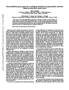
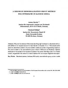
where Θ(t) denotes Heaviside’s step function. Mathematically, its origin is that the sign of t determines whether the integration contour is to be closed in the upper or lower frequency half plane. Physically, it expresses causality: the unidirectional propagator only connects earlier φ¯ fields to later φ fields (as advertised before in section 3.3). Since there exists no earlier source of φ¯ fields, the time integral in S0 may as well be extended from [0, tf ] to all times, as claimed above. Obviously, for multi-species systems there is a distinct propagator of the form (47), (48) for each particle type. The vertices in the Feynman diagrams originate from the perturbative expansion of exp(−S + S0 ). For example, the term λi φ¯i φk in the action (38) requires k incoming propagators, that is, averages connecting k earlier φ¯ fields to the k later φ ‘legs’ attached to the vertex, and i outgoing propagators, each of which links a φ¯ to a later φ field. The diagrammatic representation of the propagator and some vertices is depicted in figure 1. Propagators attach to vertices as distinguishable objects, which implies that a given diagram will come with a multiplicative combinatorial factor counting the number of


−λ1

time G0

−λ2 n0 (a)

(b)

−λ1

−λ21

−λ 2

−λ31

−λ 3

−λ32 (c)

22

(d)

Figure 1. Various diagrammatic components: (a) the propagator G0 and the initial density n0 , (b) vertices for 2A → ℓA, (c) vertices for 3A → ℓA, and (d) vertices for branching reactions, such as A → 2A. Our convention throughout is that time increases to the left.

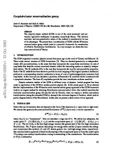
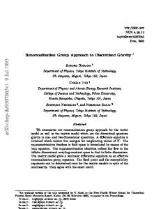
ways to make the attachments. (Note that we do not follow the convention of defining appropriate factorials with the nonlinear couplings in the action to partially account for this attachment combinatorics.) Any contribution of order m in the coupling λi is represented by a Feynman graph with m corresponding vertices. Moreover, if we are interested in the perturbation expansion for cumulants only, we merely need to consider fully connected Feynman diagrams, whose vertices are all linked through propagator lines. Lastly, the so-called vertex functions are given in terms of one-particle irreducible diagrams that do not separate into disjoint subgraphs if one propagator line is ‘cut’. ¯ = 0)] The perturbative expansion of the initial state contribution exp[−n0 φ(t creates φ¯ fields at t = 0. A term of order nm 0 comes with a factor of 1/m!, but will have m! different ways to connect the initial φ¯ fields to the corresponding Feynman graph, so the end result is that these factorials always cancel for the initial density. A similar cancellation of factorials happens for the vertices; for example, a term of order λm 1 does have the 1/m! cancelled by the number of permutations of the m λ1 vertices in the diagram. Notice, however, these combinatorial factors are distinct from those that arise from the different possibilities to attach propagators. Since the systems of interest are frequently translationally invariant (in space and time), the mathematical expressions represented by the Feynman graphs are often most conveniently evaluated in Fourier space. To calculate, say, the mean particle density hφ(t)i according to Eq. (31), one needs diagrams with a single φ field at time t which terminates the graph on the left. All diagrams that end in a single propagator line will thus contribute to the density, see figure 2. Since hφ(t)i is spatially uniform, the final propagator must have p = 0. Similarly, in momentum space the initial density terms ¯ = 0, t = 0), so the propagators connected to these also come with are of the form n0 φ(p zero wavevector. The λi vertices are to be integrated over position space, which creates a wavevector-conserving δ function. Diagrams that contain loops may have ‘internal’ propagators with p 6= 0, but momentum conservation must be satisfied at each vertex. These internal wavevectors are then to be integrated over, as are the internal time or frequency arguments. To illustrate this procedure, consider the second graph in the first row, and the first

Renormalization Group Methods for Reaction-Diffusion Problems + +

+ +

+

+ ... +

+

23

+

...

...

Figure 2. Feynman graphs that contribute to the mean particle density for the pair annihilation and coagulation reactions A + A → 0 and A + A → A. The first row depicts tree diagrams, the second row one-loop diagrams, and the third row two-loop diagrams.

diagram in the second row of figure 2, to whose loop we assign the internal momentum label p: I02 = I12 = ×

Z

t

0

Z

Z

0

t

dt1 G0 (0, t − t1 ) (−λ1 ) G0 (0, t1 )2 n20 , dt2

Z

t2

0

(49)

dt1 G0 (0, t − t2 ) (−λ1 )

dd p 2 G0 (p, t2 − t1 ) G0 (−p, t2 − t1 ) (−λ2 ) G0 (0, t1 )2 n20 d (2π)

(50)

(the indices here refer to the number of loops and the factors of initial densities involved, respectively). The factor 2 in the second contribution originates from the number of distinguishable ways to attach the propagators within the loop. Noting that G0 (p = 0, t > 0) = 1, and that the required p integrations are over Gaussians, these expressions are clearly straightforward to evaluate, I02 = −λ1 n20 t ,

I12 =

8λ1 λ2 n20 t2−d/2 (8πD)d/2 (2 − d)(4 − d)

(51)

(for d 6= 2, 4). Consequently, the effective dimensionless coupling associated with the loop in the second diagram is proportional to (λ2 /Dd/2 ) t1−d/2 . Hence, in low dimensions d < 2, the perturbation expansion is benign at small times, but becomes ill-defined as t → ∞, whereas the converse is true for d > 2. In two dimensions, the effective coupling diverges as (λ2 /D) ln(Dt) for both t → 0 and t → ∞. The ‘ultraviolet’ divergences for d ≥ 2 in the short-time regime are easily cured by introducing a short-distance cutoff in the wavevector integrals. This is physically reasonable since such a cutoff was anyhow originally present in the form of the lattice spacing (or particle capture radius). The fluctuation contributions will then explicitly depend on this cutoff scale. Thus, in dimensions d > dc = 2, perturbation theory is applicable in the asymptotic limit; this implies that the overall scaling behavior of the parameters of the theory cannot be affected by the analytic loop corrections, which can merely modify amplitudes. In contrast, the physically relevant ‘infrared’ divergences (in the long-time, long-distance limit) in low dimensions d ≤ 2 are more serious and render a ‘naive’ perturbation series meaningless. However, as will be explained in the


24

following subsections, via exploiting scale invariance and the exact structure of the renormalization group, one may nevertheless extract fluctuation-corrected power laws by means of the perturbation expansion. =

+

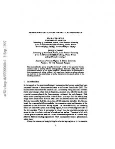
Figure 3. Graphical representation of the Dyson equation for the particle density in the A + A → 0 and A + A → A reactions.

Feynman graphs that contain no loops are called tree diagrams. For the particle density calculation illustrated in figure 2, these tree diagrams are formed with only λ1 and n0 vertices, and we denote the sum of all those tree contributions by atr (t). For example, for the A + A → (0, A) pair reactions, we may construct this entire series iteratively to all orders as shown graphically in figure 3. Thus we arrive at a selfconsistent Dyson equation for the particle density. More generally, for the single-species reactions kA → ℓA with ℓ < k the vertex on the right-hand side is connected to k full tree density lines. Since all propagators in tree diagrams come with p = 0, the corresponding analytical expression for the Dyson equation reads atr (t) = n0 − λ1

Z

0

t

dt′ atr (t′ )k .

(52)

Upon taking a time derivative, this reduces to the mean-field rate equation (1), with the correct initial condition. Furthermore, λ1 = (k − ℓ)λ0 , i.e., the rate constant is properly proportional to the number of particles removed by the reaction. Evidently, therefore, the tree-level approximation is equivalent to simple mean-field theory, and any fluctuation corrections to the rate equation must emerge from Feynman graphs that incorporate higher-order vertices λi with i > 1, i.e., diagrams with loops. We note that the mean-field rate equations also follow from the stationarity conditions, i.e., the ‘classical field equations’, for the action S (regardless of performing any field shifts). For example, taking δS/δφ = 0 = δS/δ φ¯ for the action (38) results in φ¯ = 0 and φ = atr (t). Following up on our earlier discussion, we realize that the loop fluctuation contributions cannot alter the asymptotic power laws that follow from the tree diagrams in sufficiently large dimensions d > dc , where mean-field theory should therefore yield accurate scaling exponents. However, note that, for d > dc , there will generally be non-negligible and non-universal (depending on the ultraviolet cutoff) fluctuation corrections to the amplitudes. Recall that the (upper) critical dimension dc can be readily determined as the dimension where the effective coupling associated with loop integrals becomes dimensionless. 4.2. Renormalization As we have seen in the above example (50), when one naively tries to extend the diagrammatic expansion beyond the tree contributions to include the corrections due


25

to loop diagrams, one encounters divergent integrals. We are specifically interested in the situation at low dimensions d ≤ dc : here the infrared (IR) singularities (apparent as divergences as external wavevectors p → 0 and either t → ∞ or ω → 0) emerging in the loop expansion indicate substantial deviations from the mean-field predictions. Our goal is to extract the correct asymptotic power laws associated with these ‘physical’ infrared singularities in the particle density and other correlation functions. To this end, we shall turn to our advantage the fact that power laws reflect an underlying scale invariance in the system. Once we have found a reliable method to determine the behavior of any correlation function under either length, momentum, or time scale transformations, we can readily exploit this to construct appropriate scaling laws. There exist well-developed tools for the investigation and subsequent renormalization of ultraviolet (UV) singularities, which stem from the large wavenumber contribution to the loop integrals. In our models, these divergences are superficial, since we can always reinstate short-distance cutoffs corresponding to microscopic lattice spacings. However, any such regularization procedure introduces an explicit dependence on the associated regularization scale. Since it does not employ any UV cutoff, dimensional regularization is especially useful in higher-loop calculations. Yet even then, in order to avoid the IR singularities, one must evaluate the integrals at some finite momentum, frequency, or time scale. In the following, we shall denote this normalization momentum scale as κ, associated with a length scale κ−1 , or, assuming purely diffusive propagation, time scale t0 = 1/(Dκ2 ). Once the theory has been rendered finite with respect to the UV singularities via the renormalization procedure, we can subsequently extract the dependence of the relevant renormalized model parameters on κ. This is formally achieved by means of the Callan-Symanzik RG flow equations. Precisely in a regime where scale invariance holds, i.e., in the vicinity of a RG fixed point, the ensuing ultraviolet scaling properties also yield the desired algebraic behavior in the infrared. (For a more elaborate discussion of the connections between UV and IR singularities, see Ref. [12].) The renormalization procedure itself is, in essence, a resummation of the naive, strongly cutoff-dependent loop expansion that is subsequently well-behaved as the ultraviolet regulator is removed. Technically, one defines renormalized effective parameters in the theory that formally absorb the ultraviolet poles. When such a procedure is possible — i.e., when the field theory is ‘renormalizable’, which means only a finite number of renormalized parameters need to be introduced — one obtains in this way a unique continuum limit. Examining the RG flow of the scaledependent parameters of the renormalized theory, one encounters universality in the vicinity of an IR-stable fixed point: there the theory on large length and time scales becomes independent of microscopic details. The preceding procedure is usually only quantitatively tractable at the lowest dimension that gives UV singularities, i.e., the upper critical dimension dc , which is also the highest dimension where IR divergences appear. In order to obtain the infrared scaling behavior in lower dimensions d < dc , we must at least initially resort to a perturbational treatment with respect to the marginal


26

couplings in the theory, which are dimensionless at dc (and perhaps subsequently resum the perturbation series). The scaling exponents can then be obtained in a controlled manner in a dimensional expansion with respect to the small parameter ǫ = dc − d. We can follow standard procedures (see, e.g., Refs. [70, 71, 72]) for implementing the renormalization program. First, we must identify the primitive UV divergences, the sub-components of the diagrams that are responsible for these singularities. This is most conveniently done using the vertex functions Γ(m,n) , which represent a sum of all possible one-particle irreducible Feynman graphs that are attached to n incoming and m outgoing propagator lines (of course, for a multispecies vertex function, separate indices are required for the incoming and outgoing lines of each species). In frequency and wavevector space these subdiagrams enter multiplicatively, which means that once the vertex function divergences are resolved, the general diagrammatic expansion will be well-behaved. Which vertex functions are primitively divergent can be ascertained by direct power counting: [Γ(m,n) ] = κα , where κ denotes some reference wavevector, such as the normalization scale mentioned above. The scaling dimension of the vertex function Γ(m,n) is just that of the coupling λmn from a term λmn φ¯m φn in the action, since at the tree level Γ(m,n) ∼ λmn . Loop diagram fluctuation corrections, however, require additional nonlinear couplings, which in turn determine the primitive degree of divergence for the associated momentum space integrals. We refer to the standard field theory texts for a general discussion of the ensuing vertex function dimensional analysis, but provide a brief outline of the procedure for our situation. The action S itself must be dimensionless, so any term in the integrand of S must have scaling dimension κd+2 . Consider the kA → ℓA annihilation reaction with ℓ < k. The interaction vertices λi φ¯iφk in the action (38) correspond to k incoming and i = 1 . . . k outgoing lines. With our choice of taking the continuum ¯ = κ0 . Hence we obtain limit, the scaling dimension of the fields are [φ] = κd and [φ] [Γ(i,k) ] = [λi ] = κ2−(k−1)d for all i (recall that λi ∝ λ0 of the unshifted theory). Let us now investigate the lowest-order loop correction to the vertex function Γ(i,k) , which contains k internal propagator lines, and thus is proportional to λi λk . The involved momentum integral therefore must scale as [λk ]−1 = κ(k−1)d−2 . By choosing as κ the inverse short-distance cutoff, we see that if the exponent here is non-negative, the vertex function contains a primitive UV divergence (as κ → ∞) and must be renormalized. (The converse is true for the IR singularities, which emerge in the limit κ → 0.) The l-th order corrections to the bare vertex function must scale as κl[(k−1)d−2] . Consequently, for a given k, the vertex functions Γ(i,k) become primitively UV-divergent, and increasingly so in higher loop orders, for d > dc = 2/(k − 1) for all i. The IR singularities, on the other hand, become successively worse in higher orders of the perturbation expansion for d < dc . At the critical dimension, the loop diagrams carry logarithmic UV and IR divergences, independent of the loop order. Hence this scaling discussion already reveals the upper critical dimension dc = 2 for pair annihilation and coagulation, A + A → (0, A), in agreement with our analysis following Eq. (51), whereas dc = 1 for the triplet reactions 3A → ℓA. All higher-order


27

reactions should be adequately described by mean-field theory, as represented by the tree Feynman graphs. But in general, since the assignment of scaling dimensions to the fields φ and φ¯ is somewhat arbitrary, one needs to be more careful and first determine the effective couplings in the perturbational expansion and from there infer the upper critical dimension. For example, the field theory for directed percolation, see section 6 ¯ 2 and λ21 φ¯2 φ. The effective coupling then turns below, incorporates the vertices λ12 φφ out to be the product u ∼ λ12 λ21 , whose scaling dimension is [u] = κ4−d , which indicates that actually dc = 4 in this case. Once the primitive divergences are identified, they are used to define renormalized coupling constants into which the UV singularities are absorbed. For the kA → ℓA decay reaction, this procedure is unusually simple, and in fact the entire perturbation series can be summed to all orders. First, we note that since all vertices in the action (38) have k ≥ 2 incoming lines, one cannot construct any loop diagram for the vertex function Γ(1,1) that corresponds to the inverse propagator. Hence the bare diffusion propagator (47) or (48) is not affected by fluctuations and the tree-level scaling x ∼ p−1 ∼ (Dt)1/2 remains intact [33]. The absence of field and diffusion constant renormalization in this case constitutes the fundamental reason that improved mean-field theories of the Smoluchowski type, and also simple scaling approaches, are capable of obtaining correct density decay exponents. Hence, for pair annihilation or coagulation, one would predict that the density of surviving particles at time t is given in terms of the diffusion length by a(t) ∼ x−d ∼ (Dt)−d/2 . = t2

+

+

t1 +

+ ...

Figure 4. The set of primitively divergent diagrams contributing to Γ(1,3) (t2 − t1 ) for the 3A → ℓA reaction, ℓ ≤ 2.

This leaves us with the renormalization of the vertex couplings λm , encoded in the vertex functions Γ(m,k) . Since all λm are proportional to the reaction rate λ0 , there is essentially only a single renormalized coupling gR (as is obvious if we work with the unshifted action). As a representative example, we depict the ensuing diagrammatic expansion for the case m = 1 and k = 3 in figure 4. It will be sufficient to work with p = 0. In (p, t) space we obtain explicitly Γ(m,k) (t2 − t1 ) = λm δ(t2 − t1 ) − λm λ0 I(t2 − t1 ) +

λm λ20

Z

t2

t1

dt′ I(t2 − t′ )I(t′ − t1 ) − . . . ,

(53)

where we have used λk = λ0 , and I(t) is given by the following integral with k − 1 loops over k propagators: I(t) = k!

Z Y k

i=1

!

!

X k k X d d pi 2 d Dpi t = Bk (Dt)−d/dc , pi exp − (2π) δ (2π)d i=1 i=1

(54)


28

with Bk = k! k −d/2 (4π)−d/dc and dc = 2/(k − 1). Taking the Laplace transform e (m,k) (s) = Γ

Z

0

∞

Γ(m,k) (t) e−st dt ,

(55)

the convolution theorem renders (53) into a geometric sum: λm e e (m,k) (s) = , I(s) = Bk Γ(ǫ/dc )D −d/dc s−ǫ/dc , Γ e 1 + λ0 I(s)

(56)

e where ǫ = dc − d, and Γ(x) is Euler’s gamma function. For ǫ > 0, the loop integral I(s) displays the expected IR divergence as s → 0. On the other hand, the UV singularity (for finite s) at dc appears as an ǫ pole in the gamma function Γ(ǫ/dc ) ∝ dc /ǫ. Recall that the bare effective coupling λ0 /D has scaling dimension κ2−(k−1)d = κ2ǫ/dc . Hence we may introduce the dimensionless parameter g0 = (λ0 /D) κ−2ǫ/dc with some arbitrary momentum scale κ. Next we define its renormalized counterpart by e (k,k) at vanishing external wavevectors and Laplace the value of the vertex function Γ argument s = 1/t0 = Dκ2 , which sets our normalization point. Thus,

e (k,k) (s) gR = Γ

s=Dκ2

κ−2ǫ/dc /D = Zg g0 ,

Zg−1 = 1 + g0 Bk Γ(ǫ/dc )

(57)

according to Eq. (56). Formally, a perturbative expansion in terms of g0 can be readily exchanged for an expansion in gR by straight substitution g0 = gR /[1 − gR Bk Γ(ǫ/dc )]. As ǫ → 0, however, this substitution becomes singular, since the multiplicative renormalization constant Zg−1 that was introduced to absorb the UV pole diverges in this limit. It is crucial to note that the renormalized coupling explicitly depends on the normalization scale κ. Indeed, this is borne out by calculating the associated RG β function "

#

"

#

ǫ 2ǫ ∂ ǫ ∂ gR . gR = gR − − κ ln Zg−1 = 2gR − + Bk Γ 1 + βg (gR ) = κ ∂κ dc ∂κ dc dc

(58)

Notice that βg , here computed to all orders in perturbation theory, is regular as ǫ → 0 when expressed in terms of renormalized quantities. For the simple annihilation models, the β function is exactly quadratic in gR , which is not typical and is due to the geometric sum in the primitively divergent vertex function, which reduces the fluctuation contributions effectively to the one-loop graph. Eq.(58) has the standard structure that the linear coefficient is of order ǫ = dc − d while the quadratic coefficient is order unity. The theory is manifestly scale-invariant (independent of κ) at either gR = 0 (which here corresponds to pure diffusion, no reactions) or at the special fixed-point value for the coupling given by the nontrivial zero of the β function gR∗ = [Bk Γ(ǫ/dc )]−1 ,

(59)

which is of order ǫ. We remark that the above renormalization structure directly applies to multispecies annihilation reactions as well. Consider, for example, the action (42) for A + B → 0. Once again, the vertices permit no propagator renormalization, and the perturbation expansion for the vertex functions that define the renormalized reaction rate takes the same form as in figure 4, with incoming A and B lines, and the series of internal loops


29

formed with precisely these two distinct propagators. Consequently, we just recover the previous results (57), (58), and (59) with k = 2. 4.3. Callan-Symanzik equation and loop expansion for the density In order to employ the renormalization group machinery to obtain asymptotic (longtime, large-distance) expressions for the particle density and its correlations, we next develop the Callan-Symanzik equation for the density. By means of perturbation theory in the IR-finite regime and the subsequent substitutions of gR for λ0 , the density can be calculated as an explicit function of time t, initial density n0 , diffusion constant D, renormalized coupling gR , and arbitrary normalization point κ (or the equivalent time scale t0 = 1/Dκ2 ). Since κ does not appear at all in the unrenormalized theory, we must have κ da(t, n0 , D, λ0)/dκ = 0 for the particle density at fixed bare parameters, or equivalently, after rewriting in terms of the renormalized density, "

#

∂ ∂ a(t, n0 , D, κ, gR) = 0 + βg (gR ) κ ∂κ ∂gR

(60)

with the β function (58). Yet dimensional analysis tells us that a(t, n0 , D, κ, gR ) = κd a ˆ(t/t0 , n0 /κd , gR ), reducing the number of independent variables to three. Consequently, Eq. (60) yields the Callan-Symanzik (CS) equation "

#

∂ ∂ ∂ − dn0 + βg (gR ) + d a(t, n0 , D, κ, gR) = 0 . 2Dt ∂(Dt) ∂n0 ∂gR

(61)

This partial differential equation is solved by the standard method of characteristics, where one introduces a flow parameter via κ → κℓ. The IR asymptotic region then corresponds to ℓ → 0. For our purposes, it is most convenient to directly employ (κℓ)2 = 1/Dt or ℓ2 = t0 /t. Thereby we find

a(t, n0 , t0 , gR ) = (t0 /t)d/2 a n ˜ 0 (t), g˜R (t) , with the running initial density

(62)

n ˜ 0 (t) = (t/t0 )d/2 n0 ,

(63)

and the running coupling g˜R defined by the solution of the characteristic equation d˜ gR (ℓ) d˜ gR (t) = −2t = βg (˜ gR ) , g˜R (ℓ = 1) = g˜R (t = t0 ) = gR . (64) dℓ dt The method of characteristics requires a known value of the function, in this case the density, for some value of the running parameters. Since we chose the normalization point s = 1/t0 > 0 outside the IR-singular region, we may use perturbation theory to calculate the right-hand side of Eq. (62). The Callan-Symanzik equation then allows us to transport this result into the perturbatively inaccessible asymptotic region. Because of the simple form of the β function (58), the running coupling can be found exactly by integrating the flow equation (64): ℓ

g˜R (t) =

gR∗

"

g ∗ − gR 1+ R gR

t0 t

ǫ/dc #−1

(ǫ 6= 0) .

(65)


30

Thus we see for ǫ > 0 that the running renormalized coupling approaches the RG fixed point (59) as t → ∞, independent of its initial value gR . Thus, universal behavior emerges in the asymptotic regime, whose scaling properties are governed by the IRstable fixed point gR∗ . Therefore an expansion in powers of g0 is converted, via the CS equation, to an expansion in powers of ǫ. For this purpose, we merely need to invert Eq. (57) to find g0 in terms of gR : g0 = gR /[1 − gR /gR∗ ] = gR + gR2 /gR∗ + . . .. Notice that gR = gR∗ formally corresponds to g0 ∼ λ0 /D = ∞, i.e., the annihilation reactions are indeed diffusion-limited. Above the critical dimension (ǫ < 0), g˜R (t) → 0 algebraically ∼ t−|ǫ|/dc , whereas precisely at dc the running coupling tends to zero only logarithmically, gR (ǫ = 0) . (66) g˜R (t) = 1 + Bk gR ln(t/t0 ) We may use these findings to already make contact with both the rate equation and Smoluchowski approximations. For d > dc , the effective reaction rate λ(t) ∼ D(κℓ)2ǫ/dc g˜R (ℓ) = D(Dt)−ǫ/dc g˜R (t) → const. asymptotically, as implicitly taken for granted in mean-field theory. Below the critical dimension, however, λ(t ≫ t0 ) ∼ D(Dt)−ǫ/dc gR∗ or its density-dependent counterpart λ(a) ∼ Da2ǫ/(d dc ) decrease precisely as in the Smoluchowski approach. At dc , we have instead λ(t) ∼ D/ ln(t/t0 ) or λ(a) ∼ D/ ln(1/a). Replacing λ → λ(t) or λ(a) in the mean-field rate equations (1) then immediately yields the results (6) for k = 2, whereas a(t) ∼ [ln(Dt)/Dt]1/2 for k = 3 at dc = 1.

(a)

(d)

(b)

(e)

(c)

(f)

(g)

Figure 5. One-loop and two-loop Feynman diagrams for the particle density, shown for the pair annihilation reaction k = 2.

While we have now established a systematic expansion in terms of gR , a perturbative calculation in powers of n0 is not useful, since n ˜ 0 (t) diverges for t ≫ t0 , Eq. (63). It is thus imperative to calculate to all orders in the initial density n0 . To this end, we proceed to group the Feynman graphs for the particle density according to the number of closed loops involved. First, we obtain the tree diagrams represented by the Dyson equation in figure 3. When substituted into the right-hand side of Eq. (62) the limit n ˜ 0 → ∞ will give a finite result, with leading corrections ∼ 1/˜ n0 ∼ t−d/2 that vanish asymptotically. Explicitly, replacing the bare with flowing renormalized quantities in Eqs. (62) and (2) at the RG fixed point gives n0 → Aekℓ (Dt)−d/2 , (67) a(t) = 2/dc ∗ d /2 d/d c c [1 + n0 (k − 1)(k − ℓ)gR (Dt) ] with universal amplitude Aekℓ = [(k − 1)(k − ℓ)gR∗ ]−1/(k−1) .


31

Next, we consider one- (a) and two-loop (b)–(g) diagrams for the density, depicted in figure 5 (all for the case k = 2, but the generalization to arbitrary k is obvious). In order to sum over all powers of n0 , the propagators in these diagrams are replaced with response functions, which include sums over all tree-level dressings. These are depicted in figure 6, along with the Dyson equation they satisfy. For d ≤ dc each vertex coupling asymptotically flows to the O(ǫ) fixed point (59), so the loop expansion corresponds to an ordering in successive powers of ǫ = dc − d. However, each order of the expansion, under RG flow, comes in with the same t−d/2 time dependence. Thus, the loop expansion confirms that the exponent is given explicitly by the tree-level result, and provides an epsilon expansion for the amplitude of the density decay. k

t2

=

+

=

+

+

+ ...

t1

Figure 6. Response function for k=2

As mentioned above, the very same renormalizations hold for multi-species annihilation reactions, for example the pair process A + B → 0. Consequently, in the case of unequal initial A and B densities (with a0 < b0 , say) in dimensions d > dc = 2, the mean-field result that the minority species vanishes exponentially a(t) ∼ exp(−λt) is recovered, whereas for d < 2 the direct replacement λ → λ(t) ∼ D(Dt)−1+d/2 correctly yields a stretched exponential decay a(t) ∼ exp[−const. (Dt)d/2 ], while at dc = 2 the process is slowed down only logarithmically, a(t) ∼ exp[−const. Dt/ ln(Dt)]. The asymptotic B particle saturation density is approached with the same time dependences. The amplitudes in the exponentials were computed exactly by other means in dimensions d ≤ 2 by Blythe and Bray [19]. 5. Further Applications Now that we have established the basic field-theoretic RG machinery necessary to systematically compute exponents and amplitudes, we can summarize some more sophisticated applications. We deal first with systems without phase transitions, before moving on in section 6 to describe reaction-diffusion systems that display nonequilibrium phase transitions between active and absorbing states. Our aim in this section will be to give a brief outline of the results available using RG methods, rather than to delve too deeply into calculational details. 5.1. Single-species reactions • The kA → ℓA reaction with ℓ < k: The RG treatment for the general single-species annihilation reactions kA → ℓA (ℓ < k) was explicitly covered in the previous sections. The upper critical dimension of these


32

reactions is dc = 2/(k − 1), and we note in particular that the reactions A + A → 0 and A + A → A are in the same universality class [33]. We also emphasize again that, for d ≤ dc , the amplitudes and exponents are universal, independent of the initial conditions (apart from highly specialized initial conditions, such as those in Ref. [73], where the particles were initially positioned in pairs). • A + A → (0, A) with particle input 0 → A: Droz and Sasvári [74] studied the steady state of the combined A + A → (0, A) and 0 → A reactions, focusing particularly on how the density scales with J, the particle input rate. This process appears as an interaction J φ¯ in the action. Power counting gives [J] = κ2+d and straightforward arguments show that for d < dc = 2, and for sufficiently small values of J, the density scales as J d/(d+2) , and that the characteristic relaxation time behaves as τ ∼ J −2/(d+2) . Finally, these findings were combined to reproduce the standard density scaling as t−d/2 . Rey and Droz extended this approach to provide explicit perturbative calculations of the density scaling function [75]. • Disordered systems: Another important variation on these simple reaction-diffusion models is to include quenched disorder in the transport. Various models of quenched random velocity fields in the A + A → 0 reaction have been investigated using RG techniques, including uncorrelated (Sinai) disorder [76] and also long-ranged correlated potential disorder [77]. We consider first the case of (weak) Sinai disorder, with velocity correlator hv α (x)v β (y)i = ∆δα,β δ(x−y) analyzed by Richardson and Cardy [76]. An effective action is found by averaging over this disorder, after which one must renormalize the disorder strength and diffusion constant in addition to the reaction rate. Unlike the case of pure diffusive transport, it turns out that the amplitude for the asymptotic density decay rate as a function of time is nonuniversal for d < 2: n ∼ Cd t−d/z , with z = 2 + 2ǫ2 + O(ǫ3 ) and ǫ = 2 − d, but where Cd must be nonuniversal on dimensional grounds. It is only when rewriting the density as a function of the disorder-averaged diffusion length that a universal scaling relation emerges: n ∼ Bd hr 2 i−d/2 , where Bd is universal. Results were also obtained for d = 2, where the effects of the uncorrelated disorder are not strong (only the amplitude, but not the exponent, of the asymptotic density decay is altered). Interestingly, for weak disorder, it was found that the amplitude of the density decay is reduced, implying that the effective reaction rate is faster than for the case of purely diffusing reactants. Physically, this results from the disorder ‘pushing’ particles into the same region of space, thus speeding up the kinetics. Theoretically, this originates in a disorder-induced renormalization of the reaction rate. However, as the disorder is increased it was also shown that the reaction rate would then begin to decrease. This stems from a disorder-induced renormalization of the diffusion, which works to slow the kinetics, i.e. operates in the opposite direction to the disorder-induced reaction rate renormalization. The related case of long-ranged potential disorder, where the random velocity field


33

can be considered as the gradient of a random potential, was analyzed using RG methods in two dimensions by Park and Deem [77]. In this case, rather more drastic effects were found, with an altered decay exponent from the case of purely diffusing reactants. Physically, this results from the different nature of the disordered landscape [78], where for long-ranged potential disorder, but not of the Sinai type, deep trapping wells exist where, in order to escape the trap, a particle must move in an unfavorable direction. Park and Deem employed replicas to analyze the effect of long-ranged disorder, where the correlation function of the quenched random potential behaves as γ/k 2 . They obtained that the asymptotic density decay was modified to tδ−1 , where δ is defined in the absence of reaction by the anomalous diffusion relation hr(t)2 i ∼ t1−δ . Here, δ was found to be a nonuniversal exponent depending on the strength of the disorder. The amplitude of the decay also turned out to be a nonuniversal quantity. We also mention that ‘superfast’ reactivity has been found in d = 2 for the A + A → 0 reaction in a model of turbulent flow with potential disorder [79]. This case was also investigated numerically [80]. RG methods indicated that this regime persists in a more realistic time-dependent model for the random velocity field [80]. The case of A + A → 0 also in a time-dependent random velocity field, but generated now by a stochastically forced Navier-Stokes equation, was considered in Ref. [81]. • Lévy flights in reactive systems: Replacing diffusive propagation with long-ranged Lévy flights constitutes another important modification to the dynamics of reactive systems. Such Lévy flights are characterized by a probability for a particle’s jump length ℓ decaying for large ℓ as P ∼ ℓ−d−σ . For σ < 2 this results in a mean-square displacement in one dimension growing as t1/σ , faster than the t1/2 law of diffusion. Naturally, one expects that altering the dynamics of the system in this way will modify the kinetics, as one is effectively making the system better mixed with decreasing σ. The propagator for Lévy processes becomes G0 (p, ω) = (−iω+DL pσ )−1 , meaning that time scales acquire scaling dimension κ−σ rather than κ−2 (for σ < 2). Consequently, power counting for the A + A → (0, A) reaction gives [λ] = κσ−d , implying that dc = σ. Once again only the reaction rate is renormalized, which then flows to an O(ǫ = σ−d) fixed point under the RG. Dimensional analysis subseqently fixes the asymptotic density decay rate as t−d/σ , for d < σ [82]. Note that the upper critical dimension is now a function of the Lévy index σ. This feature has been exploited by Vernon [83] to compute the density amplitude for the A + A → 0 reaction with Lévy flights to first order in ǫ = σ − d. σ was then set to be slightly larger than unity and the behavior of the system was studied numerically in d = 1. This ensures that ǫ = σ − d is a genuinely small expansion parameter (i.e., ǫ ≪ 1) in the physical dimension d = 1. This contrasts with the case of A + A → 0 with standard diffusion where, in order to access d = 1, ǫ = 2 − d must be set to unity. As we have seen, in that situation the expansion for the density amplitude agrees only rather poorly with numerics [20]. However, for the Lévy flight case, Vernon demonstrated that the accuracy of the expansion indeed improves with decreasing ǫ (i.e. decreasing


34

σ towards unity). This ability to vary the value of dc has also been used to probe the behavior of directed percolation and branching-annihilating random walks [82, 84, 85], see section 6 below. We also mention that the reaction A + A → 0 with Lévy flights and quenched disorder was studied using RG methods in Ref. [86]. Finally, the authors of Ref. [87] used RG techniques to investigate the case of short-ranged diffusion, but with long-ranged reactive interactions. 5.2. Two-species reactions • The homogeneous A + B → 0 reaction: The two-species decay reaction is perhaps the most relevant to chemical systems. It is also considerably more complicated to analyze, since the A + B → 0 pair annihilation process leaves the local density difference field a − b unchanged. This conservation law provides a slow mode in the dynamics that is crucial in determining the long-time behavior of the system. We consider first the case where the A and B particles are initially mixed together throughout the system. If their initial densities are unequal, say b0 > a0 , the asymptotic dynamics will approach a steady concentration of b0 − a0 of B particles, with very few isolated A particles suriving. In this situation, exact results indicate an exponentially decaying A particle density for d > 2, logarithmic corrections √ to an exponential in d = 2, and a stretched exponential exp(−c t) form for d = 1 [16, 18, 19], where c is a constant. As briefly discussed in section 4.3 above, these results correspond in the RG framework to the standard renormalization of the reaction rate. In contrast, when starting from equal initial densities, the fluctuations in the initial conditions for the difference field a − b decay to zero slowly, by diffusion. This case was studied by Toussaint and Wilczek [29] based on the idea that after a time t, on length scales shorter than the diffusion length ld ∼ t1/2 only whichever of the species happened to be in the majority in that region initially will remain. In other words, the two species asymptotically segregate. Since the initial difference between the A and B particle d/2 numbers in that region is proportional to lD , this leads to an asymptotic t−d/4 decay [29]. Clearly, for d < 4, this dominates the faster t−1 mean-field density decay which assumes well-mixed reactants throughout the system’s temporal evolution. Toussaint and Wilczek explicitly calculated the amplitude for this decay under the assumption that the only relevant fluctuations are those in the initial conditions. These results were since confirmed by exact methods [16, 17, 31]. Turning to the field-theoretic RG approach, the action (42) for the process A+B → 0 contains diffusive propagators for both A and B species, possibly with unequal diffusion constants, together with the interaction vertices λ¯ aab, λ¯bab and λ¯ a¯bab. Power counting reveals [λ] = κ2−d , the same as in the A + A → 0 reaction. This implies that the upper critical dimension is dc = 2, consistent with the behavior for unequal initial densities. The renormalization of the A + B → 0 action also follows similarly to the A + A → 0 case. Surprisingly, however, a full RG calculation of the asymptotic density in the case


35

of unequal initial densities has not yet been fully carried through. For the equal density case, though, a field theory approach by Lee and Cardy is available [21]. The ToussaintWilczek analysis reveals a qualitative change in the system’s behavior in four dimensions, whereas the field theory yields dc = 2. The resolution of this issue lies in the derivation of an effective theory valid for 2 < d ≤ 4, where one must allow for the generation of effective initial (t = 0) ‘surface’ terms, incorporating the fluctuations of the initial state. Aside from this initial fluctuation term, it was shown that the mean-field rate equations suffice [21]. Using the field theory approach, Lee and Cardy were also able to demonstrate the asymptotic segregation of the A and B species, and thus provided a more rigorous justification of the Toussaint-Wilczek result for both the t−d/4 density decay and amplitude for 2 < d < 4. For d ≤ dc = 2, a full RG calculation becomes necessary. Remarkably, comparisons with exact results for the decay exponent in one dimension [16, 17, 31] show that this qualitative change in the system does not lead to any modification in the form of the asymptotic density decay exponent at d = 2 (and so very unlike the case of unequal initial denities). However, actually demonstrating this using field theory methods has not yet been accomplished, since this would involve a very difficult non-perturbative sum over the initial ‘surface’ terms. Lastly, we also mention related work by Sasamoto and coworkers [88] where the mA + nB → 0 reaction was studied using field-theoretic techniques, by methods similar to those of Ref. [21]. These authors also found a t−d/4 decay rate independent of m and n (provided both are nonzero), valid for d < 4/(m + n − 1). • The segregated A + B → 0 reaction, reaction zones: Two-species reactions can also be studied starting from an initial condition of a segregated state, where a (d − 1)-dimensional surface separates the two species at time t = 0. Later, as the particles have an opportunity to diffuse into the interface, a reaction zone forms. Gálfi and Racz first studied these reaction zones within the local mean-field equations, and were able to extract some rich scaling behavior: the width of the reaction region grows as w ∼ t1/6 , the width of the depletion region grows, as might be expected, as t1/2 , and the particle densities in the reaction zone scale as t−1/3 [30]. Redner and Ben-Naim [89] proposed a variation of this model where equal and opposite currents of A and B particles are directed towards one another and a steadystate reaction zone is formed. In this case it is of interest to study how the various lengths scale with the particle current J. Within the local mean-field equations they found that the width of the reaction region grows as w ∼ J −1/3 , whereas the particle densities in the reaction zone scale as J 2/3 . The above initially segregated system may be directly related to this steady-state case by observing that, in the former, the depletion region is asymptotically much larger than the reaction zone itself. This means there is a significant region where the density evolves only by diffusion, and goes from a constant to zero over a range L ∼ t1/2 . Since J ∼ −∇a, we find J ∼ t−1/2 , which may be used to translate results between these two cases. Cornell and Droz [90] extended the analysis of the steady-state problem beyond the


36

mean field equations and, with RG motivated arguments, conjectured a reaction zone width w ∼ J −1/(d+1) for the case d < 2. Lee and Cardy confirmed this result using RG methods [91]. The essential physics here is that the only dimensional parameters entering the problem are the reaction rate and the current J. However, for d ≤ 2, RG methods demonstrate that the asymptotics are independent of the reaction rate. In that case, dimensional analysis fixes the above scaling form (with logarithmic corrections in d = 2 [21]). Howard and Cardy [92] provided explicit calculations for the scaling functions. However, numerical investigations of the exponent of the reaction zone width revealed a surprisingly slow convergence to its predicted value w ∼ J −1/2 ∼ t1/4 in d = 1 [93]. The resolution of this issue was provided in Ref. [94], where the noiseinduced wandering of the front was considered (in contrast to the intrinsic front profile analyzed previously). There it was shown that this noise-induced wandering dominates over the intrinsic front width and generates a multiplicative logarithmic correction to the basic w ∼ J −1/2 ∼ t1/4 scaling in d = 1. Remarkably, one can also study the reaction zones in the initially mixed system with equal initial densities, since it asymptotically segregates for d < 4 and spontaneously forms reaction zones. As shown by Lee and Cardy [91], if one assumes that in the depletion regions, where only diffusion occurs, the density goes from the bulk value t−d/4 to zero in a distance of order t1/2 , the current scales as J ∼ t−(d+2)/4 . From this the scaling of the reaction zone width with time immediately follows. As d → 4 from below, the reaction zone width approaches t1/2 , i.e., the reaction zone size becomes comparable to the depletion zone, consistent with the breakdown of segregation. This analysis also reveals the true critical dimension dc = 2, with logarithmic corrections w ∼ (t ln t)1/3 arising from the marginal coupling in d = 2 [21]. • Inhomogeneous reactions, shear flow and disorder: One important variant of the A+B → 0 reaction, first analyzed by Howard and Barkema [95], concerns its behavior in the linear shear flow v = v0 yˆ x, where x ˆ is a unit vector in the x-direction. Since the shear flow tends to enhance the mixing of the reactants, we expect that the reaction kinetics will differ from the homogeneous case. A simple generalization of the qualitative arguments of Toussaint and Wilczek shows that this is indeed the case. The presence of the shear flow means that in volumes smaller than (Dt)d/2 [1 + (v0 t)2 /3]1/2 only the species which was initially in the majority of that region will remain. Hence, we immediately identify a crossover time tc ∼ v0−1 . For t ≪ tc the shear flow is unimportant and the usual t−d/4 density decay is preserved. However for t ≫ tc , we find a t−(d+2)/4 decay holding in d < 2. Since d = 2 is clearly the lowest possible dimension for such a shear flow, we see that the shear has essentially eliminated the non-classical kinetics. These arguments can be put on a more concrete basis by a field-theoretic RG analysis [95], which shows the shear flow adds terms of the form a ¯v0 y∂x a and ¯bv0 y∂x b to the action. The effect of these contributions can then be incorporated into modified propagators, after which the analysis proceeds similarly to the homogeneous case [21].


37

The related, but somewhat more complex example of A + B → 0 in a quenched random velocity field was considered by Oerding [96]. In this case it was assumed that the velocity at every point r = (x, y) of a d-dimensional system was either parallel or antiparallel to the x axis and depended only on the coordinate perpendicular to the flow. The velocity field was modeled by quenched Gaussian random variables with zero mean, but with correlator hv(y)v(y′)i = f0 δ(y − y′ ). In this situation, qualitative arguments again determine the density decay exponent. Below three dimensions, a random walk in this random velocity field shows superdiffusive behavior in the x-direction [97]. The mean-square displacement in the x direction averaged over configurations of v(y) is hx2 i ∼ t(5−d)/2 for d < 3. Generalizing the Toussaint-Wilczek argument then gives an asymptotic density decay of t−(d+3)/8 . In this case, the system still segregates into A and B rich regions, albeit with a modified decay exponent for d < 3. However, to proceed beyond this result, Oerding applied RG methods to confirm the decay exponent and also to compute the amplitude of the density decay to first order in ǫ = 3 − d [96]. The analysis proceeds along the same lines as the homogeneous case [21], particularly in the derivation of effective ‘initial’ interaction terms, although care must also be taken to incorporate the effects of the random velocity field, which include a renormalization of the diffusion constant. Lastly, we mention work by Deem and Park, who analyzed the properties of the A + B → 0 reaction using RG methods in the case of long-ranged potential disorder [98], and in a model of turbulent flow [79]. • Reversible reactions, approach to equilibrium: Rey and Cardy [99] studied the reversible reaction-diffusion systems A + A ⇀ ↽ C and A + B ⇀ ↽ C using RG techniques. Unlike the case of critical dynamics in equilibrium systems, the authors found that no new nontrivial exponents were involved. By exploiting the existence of conserved quantities in the dynamics, they found that, starting from random initial conditions, the approach of the C species to its equilibrium density takes the form At−d/2 in both cases and in all dimensions. The exponent follows directly from the conservation laws and is universal, whereas the amplitude A turns out to be model-dependent. Rey and Cardy also considered the cases of correlated initial conditions and unequal diffusion constants, which exhibit more complicated behavior, including a nonmonotonic approach to equilibrium. 5.3. Coupled reactions without active phase The mixed reaction-diffusion system A+A → 0, A+B → 0, B +B → 0 was first studied using field-theoretic RG methods by Howard [57], motivated by the study of persistence probabilities (see section 5.4). The renormalization of the theory proceeds again similar to the case of A + A → 0: only the reaction rates need to be renormalized, and this can be performed to all orders in perturbation theory. For d ≤ dc = 2, perturbative calculations for the density decay rates were only possible in the limit where the density of one species was very much greater than that of the other. The density decay exponent


38

of the majority species then follows the standard pure annihilation kinetics, whereas the minority species decay exponent was computed to O(ǫ = 2 − d) [57]. This oneloop exponent turned out to be a complicated function of the ratio of the A and B species diffusion constants. The calculation of this exponent using RG methods has been confirmed and also slightly generalized in Ref. [100]. The above mixed reactiondiffusion system also provides a good testing ground in which to compare RG methods with the Smoluchowski approximation, which had earlier been applied to the same multispecies reaction-diffusion system [101]. This is a revealing comparison as the value of the minority species decay exponent is non-trivial for d ≤ 2, and is no longer fixed purely by dimensional analysis (as is the case for the pure annihilation exponent for d < 2). This difference follows from the existence of an additional dimensionless parameter in the multi-species problem, namely the ratio of diffusion constants. Nevertheless, in this case, it turns out that the Smoluchowski approximation decay exponent is identical to the RG-improved tree level result, and provides rather a good approximation in d = 1 [101, 57]. However, this is not always the case for other similar multi-species reactiondiffusion models, where the Smoluchowski approximation can become quite inaccurate (see Refs. [57, 100] for more details). The same system but with equal diffusion constants was also analyzed using RG methods in Ref. [102], as a model for a steric reaction-diffusion system. As pointed out in Refs. [57, 103], this model has the interesting property that at large times for d ≤ dc = 2, the densities of both species always decay at the same rate, contrary to the predictions of mean-field theory. This result follows from the indistinguishability of the two species at large times: below the upper critical dimension, the reaction rates run to identical fixed points. Since the diffusion constants are also equal there is then no way to asymptotically distinguish between the two species, whose densities must therefore decay at the same rate. The same set of reactions, with equal diffusion constants, was used to study the application of Bogolyubov’s theory of weakly nonideal Bose gases to reaction-diffusion systems [104]. Related models were studied in the context of the mass distribution of systems of aggregating and diffusing particles [105, 56]. In the appropriate limit, the system of Ref. [56] reduced to the reactions A + A → A and A + B → 0. Progress could then be made in computing to O(ǫ = 2−d) the form of the large-time average mass distribution, for small masses. Comparisons were also made to Smoluchowski-type approximations, which failed to capture an important feature of the distribution, namely its peculiar form at small masses, referred to by the authors of Ref. [56] as the Kang-Redner anomaly. This failure could be traced back to an anomalous dimension of the initial mass distribution, a feature which, as discussed in section 2.4, cannot be picked up by Smoluchowski-type approximations. Howard and Täuber investigated the mixed annihilation / ‘scattering’ reactions A + A → 0, A + A → B + B, B + B → A + A, and B + B → 0 [23]. In this case, for d < 2, to all orders in perturbation theory, the system reduces to the single-species annihilation case. Physically this is again due to the re-entrance property of random walks: as soon as two particles of the same species approach each other,


39

they will rapidly annihilate regardless of the competing ‘scattering’ processes, which only produce particle pairs in close proximity and therefore with a large probability of immediate subsequent annihilation. Finally, we mention the multi-species pair annihilation reactions Ai + Aj → 0 with 1 ≤ i < j ≤ q, first studied by Ben-Avraham and Redner [106], and more recently by Deloubrière and coworkers [107, 108, 109]. For unequal initial densities or different reaction rates between the species, one generically expects the same scaling as for A + B → 0 asymptotically (when only the two most numerous, or least reactive, species remain). An interesting special case therefore emerges when all rates and initial densities coincide. For any q > 2 and in dimensions d ≥ 2 it was argued that particle species segregation cannot occur, and hence that the asymptotic density decay rate for equal initial densities and annihilation rates should be the same as for the single-species reaction A + A → 0. In one dimension, however, particle segregation does take place for all q < ∞, and leads to a q-dependent power law ∼ t−(q−1)/2q for the total density [107, 108, 110]. For q = 2, this recovers the two-species decay ∼ t−1/4 , whereas the single-species behavior ∼ t−1/2 ensues in the limit q → ∞ (since the probability that a given particle belongs to a given species vanishes in this limit, any species distinction indeed becomes meaningless). Other special situations arise when the reaction rates are chosen such that certain subsets of the Ai are equivalent under a symmetry operation. One may construct scenarios where segregation occurs in dimensions d > 2 despite the absence of any microscopic conservation law [109]. A variation on this model has a finite number of walkers Ni of each species Ai , initially distributed within a finite range of the origin. Attention is focused on the asymptotic decay of the probability that no reactions have occured up to time t. The case of Ni = 1 for all i reduces to Fisher’s vicious walkers [111], and the case N1 = 1 and N2 = n reduces to Krapivsky and Redner’s lion-lamb model [112]. Applying RG methods to the general case, including unequal diffusion constants for the different species, Cardy and Katori demonstrated that the probability decays as t−α({Ni }) for d < 2, and calculated the exponent to second order in an ǫ = 2 − d expansion [113]. 5.4. Persistence Persistence, in its simplest form, refers to the probability that a particular event has never occurred in the entire history of an evolving statistical system [114]. Persistence probabilities are often universal and have been found to be nontrivial even in otherwise well-understood systems. An intensively studied example concerns the zero-temperature relaxational dynamics of the Ising model, where one is interested in the persistence probability that, starting from random initial conditions, a given site has never been visited by a domain wall. In one dimension, the motion and annihilation of Ising domain walls at zero temperature is equivalent to an A+A → 0 reaction-diffusion system, where the domain walls in the Ising system correspond to the reacting particles. An exact solution exists for the persistence probability in this case [115], but, as usual, the solution


40

casts little light on the question of universality. A different approach was proposed by Cardy who studied, in the framework of the reaction-diffusion model, the proportion of sites never visited by any particle [116]. In d = 1 (though not in higher dimensions) this is the same quantity as the original persistence probability. Furthermore, since Cardy was able to employ the kind of field-theoretic RG methods discussed in this review, the issue of universality could be addressed as well. Cardy demonstrated that the probability of never finding a particle at the origin could be calculated within the field-theoretic formalism through the inclusion of an Q ˆ†0 a ˆ0 operators are associated operator product t δaˆ† aˆ0 ,0 . The subscript denotes that the a 0 with the origin, and the operator-valued Kronecker δ-function ensures that zero weight is assigned to any histories with a particle at the origin. This operator has the net effect R ¯ t′ )φ(0, t′)dt′ to the action, and the persistence probability of adding a term −h 0t φ(0, R then corresponds to the expectation value hexp(−h 0t φ(0, t′ )dt′ )i, averaged with respect to the modified action. Power counting reveals that [h] ∼ κ2−d , so this coupling is relevant for d < 2. Cardy showed that renormalization of this interaction required both a renormalized coupling hR and a multiplicative renormalization of the field φ(0, t). This results in a controlled ǫ = 2 − d expansion for the universal persistence exponent θ = 1/2 + O(ǫ) [116]. This compares to the exact result in one dimension by Derrida et al., namely θ = 3/8 [115]. An alternative approach to this problem was given by Howard [57] in the mixed two-species reaction A+ A → 0, A+ B → 0, with immobile B particles (see also section 5.3). In this case the persistence probability corresponds to the density decay of immobile B particles in d = 1, in the limit where their density is much smaller than those of the A particles. Howard’s expansion confirmed the results of Cardy and also extended the computation of the persistence probability to O(ǫ = 2 − d). The case of persistence in a system of random walkers which either coagulate, with probability (q − 2)/(q − 1), or annihilate, with probability 1/(q − 1), when they meet was also investigated using RG methods by Krishnamurthy et al. [117]. In one dimension, this system models the zero-temperature Glauber dynamics of domain walls in the q-state Potts model. Krishnamurthy et al. were able to compute the probability that a given particle has never encountered another up to order ǫ = 2 − d. A further application of field-theoretic methods to persistence probabilities was introduced by Howard and Godrèche [118] in their treatment of persistence in the voter model. The dynamics of the voter model consist of choosing a site at random between t and t + dt; the ‘voter’ on that site, which can have any of q possible ‘opinions’, then takes the opinion of one its 2d neighbours, also chosen at random. This model in d = 1 is identical to the Glauber-Potts model at zero temperature, but can also, in all dimensions, be analyzed using a system of coalescing random walkers. This again opens up the possiblity for field-theoretic RG calculations, as performed in Ref. [118]. The persistence probability that a given ‘voter’ has never changed its opinion up to time t was computed for all d ≥ 2, yielding an unusual exp[−f (q)(ln t)2 ] decay in two dimensions. This result confirmed earlier numerical work by Ben-Naim et al. [119].


41

6. Active to Absorbing State Transitions In the previous sections, we have focused on the non-trivial algebraic decay towards the absorbing state in diffusion-limited reactions of the type kA → ℓA (with k ≥ 2 and ℓ < k), and some variants thereof. Universal behavior naturally emerges also near a continuous nonequilibrium phase transition that separates an active state, with nonvanishing particle density as t → ∞, from an inactive, absorbing state. We shall see that generically, such phase transitions are governed by the power laws of the directed percolation (DP) universality class [120, 121, 8, 12]. 6.1. The directed percolation (DP) universality class A phase transition separating active from inactive states is readily found when spontaneous particle decay (A → 0, with rate µ) competes with the production process (A → A + A, branching rate σ). In this linear reaction system, a(t) = a(0) exp[−(µ − σ)t] → 0 exponentially if σ < µ. In order to render the particle density a finite in the active state, i.e., for σ > µ, we need to either restrict the particle number per lattice site (say, to 0 or 1), or add a binary reaction A + A → (0, A), with rates λ(λ′ ). The corresponding mean-field rate equation reads ∂t a(t) = (σ − µ)a(t) − (2λ + λ′ ) a(t)2 ,

(68)

which for σ > µ implies that asymptotically σ−µ , (69) a(t) → a∞ = 2λ + λ′ which is approached exponentially |a(t) − a∞ | ∼ exp[−(σ − µ)t] as t → ∞. Precisely at the transition σ = µ, Eq. (68) yields the binary annihilation / coagulation mean-field power law decay a(t) ∼ t−1 . Generalizing Eq. (68) to a local particle density and taking into account diffusive propagation, we obtain with r = (µ − σ)/D: ∂t a(x, t) = −D(r − ∇2 )a(x, t) − (2λ + λ′ ) a(x, t)2 ,

(70)

wherefrom we infer the characteristic length and diffusive time scales ξ ∼ |r|−1/2 and tc ∼ ξ 2/D ∼ |r|−1 which both diverge upon approaching the critical point at r = 0. Upon defining the critical exponents ha∞ i ∼ (−r)β ξ ∼ |r|

−ν

ha(t)i ∼ t−α

(r < 0) ,

(r = 0) ,

z

tc ∼ ξ /D ∼ |r|−zν

(r 6= 0) ,

(r 6= 0) ,

(71)

we identify the mean-field values β = 1, α = 1, ν = 1/2, and z = 2. In order to properly account for fluctuations near the transition, we apply the field theory mapping explained in section 3. The ensuing coherent-state path integral action then reads ˜ φ] = S[φ,

Z

d

d x −φ(tf ) +

Z

0

tf

h

˜ + σ(1 − φ) ˜ φφ ˜ dt φ˜ ∂t − D∇2 φ − µ(1 − φ)φ

i

˜ ˜ 2 − n0 φ(0) , −λ 1 − φ˜2 φ2 − λ′ 1 − φ˜ φφ

(72)


42

which constitutes a microscopic representation of the stochastic processes in question. ¯ Equivalently, we may consider the shifted action (with φ˜ = 1 + φ) ¯ φ] = S[φ,

Z

Z

n h

o

i

¯ 2 + (λ + λ′ )φ¯2 φ2 . (73) dd x dt φ¯ ∂t + D(r − ∇2 ) φ − σ φ¯2 φ + (2λ + λ′ )φφ

Since the ongoing particle production and decay processes should quickly obliterate any ¯ remnants from the initial state, we have dropped the term n0 φ(0), and extended the temporal integral from −∞ to ∞. The classical field equations δS/δφ = 0 (always solved by φ¯ = 0) and δS/δ φ¯ = 0 yield the mean-field equation of motion (70). Our goal is to construct an appropriate mesoscopic field theory that captures the universal properties at the phase transition. Recall that the continuum limit is not unique: We are at liberty to choose the scaling dimensions of the fluctuating fields ¯ t) and φ(x, t), provided we maintain that their product scales as a density, i.e., φ(x, ¯ = κd with arbitrary momentum scale κ. In RG terms, there exists a redundant [φφ] parameter [122] that needs to be eliminated through suitable rescaling. To this end, we ¯ t)φ(0, 0)i. note that the scaling properties are encoded in the propagator G(x, t) = hφ(x, The lowest-order fluctuation correction to the tree-level expression 1 (74) G0 (p, ω) = −iω + D(r + p2 ) is given by the Feynman graph depicted in figure 7(b, top), which involves the product ∼ −σ(2λ + λ′ ) of the two three-point vertices in (73). Similarly, the one-loop correction to either of these vertices comes with the very same factor. It is thus convenient to choose the scaling dimensions of the fields in such a manner that the three-point vertices attain identical scaling dimensions. This is q achieved via introducing new fields q ′ ¯ t) (2λ + λ )/σ and s(x, t) = φ(x, t) σ/(2λ + λ′ ), whence s¯(x, t) = φ(x, S[¯ s, s] = q

Z

d

Z

n h

o

i

d x dt s¯ ∂t + D(r − ∇2 ) s − u(¯ s − s)¯ ss + (λ + λ′ )¯ s2 s2 .

(75)

Here, u = σ(2λ + λ′ ) is the new effective coupling. Since [σ] = κ2 and [λ] = κ2−d = [λ′ ], its scaling dimension is [u] = κ2−d/2 , and we therefore expect dc = 4 to be the upper critical dimension. Moreover, [(λ + λ′ )/u] = κ−d/2 scales to zero under subsequent RG transformations: compared to u, both couplings λ and λ′ alone constitute irrelevant parameters which will not affect the leading universal scaling properties. Upon omitting these irrelevant terms, we finally arrive at the desired effective field theory action Seff [¯ s, s] =

Z

Z

n h

i

o

dd x dt s¯ ∂t + D(r − ∇2 ) s − u(¯ s − s)¯ ss .

(76)

It displays duality invariance with respect to time (rapidity) inversion, s(x, t) ↔ −¯ s(x, −t). Remarkably, the action (76) was first encountered and analyzed in particle physics under the guise of Reggeon field theory [123, 124]. It was subsequently noticed that it actually represents a stochastic (‘Gribov’) process [125, 126], and its equivalence to the geometric problem of directed percolation was established [127, 128, 120]. In directed bond percolation, randomly placed bonds connecting regular lattice sites can only be traversed in a given preferred special direction, which is to be identified with t


43

in the dynamical problem. Particle decay, coagulation, and production respectively correspond to dead ends, merging links, or branching of the ensuing percolating structures. Near the percolation threshold, the scaling properties of the critical percolation cluster are characterized by the exponents governing the divergences of the transverse correlation length ν⊥ = ν and of the longitudinal (in the t direction) correlation length νk = zν. (For more details, we refer the reader to Refs. [8, 12].) From our derivation of the effective action (76) above, it is already apparent that either pair annihilation or coagulation lead to identical critical properties. Instead of these binary reactions, we could also have employed site oocupation number restrictions to render the particle density finite in the active phase. Van Wijland has recently shown how such local constraints limiting ni to values of 0, 1 only can be implemented into the second-quantized bosonic formalism [129], thus avoiding a more cumbersome representation in terms of spin operators. The resulting action acquires exponential ˜ For the competing first-order processes A → (0, 2A) one terms for each field φ. eventually obtains ˜ φ] = Srest [φ,

Z

d

d x

Z

i

(77)

hζ(x, t) ζ(x′, t′ )i = 2sN[s]δ(x − x′ ) δ(t − t′ ) ,

(79)

h

˜ ˜ ˜ e−vφφ ˜ φφ ˜ e−2vφφ , dt −µ(1 − φ)φ + σ(1 − φ)

where we have merely written down the bulk reaction part of the action, and v is a parameter of scaling dimension [v] = κ−d which originates from taking the continuum limit. Since therefore v will scale to zero under RG transformations, we may expand the exponentials, whereupon the leading terms in the corresponding shifted action assume the form (75), with 2λ + λ′ = (2σ − µ)v ≈ σv and λ + λ′ = 4σv. Thus we are again led to the effective DP field theory action (76) (despite the formally negative value for λ). Following the procedure outlined in section 3.5 [1], we find that the field theory action (76) is equivalent to the stochastic differential equation √ (78) ∂t s = D ∇2 − r s − us2 + 2us η , √ with hηi = 0, hη(x, t) η(x′ , t′ )i = δ(x − x′ ) δ(t − t′ ), or, upon setting ζ = 2us η in order to eliminate the square-root multiplicative noise, hζi = 0, hζ(x, t) ζ(x′, t′ )i = 2us(x, t)δ(x−x′ ) δ(t−t′ ). We may view these resulting terms as representing the leadingorder contributions in a power-law expansion of the reaction and noise correlation functionals R[s] = r + us + . . . and N[s] = u + . . . with respect to the density s of activity in

∂t s = D ∇2 − R[s] s + ζ ,

which represents the general Langevin description of systems displaying active and absorbing states [12]. A factor s has been factored out of both R and N here, since the stochastic processes must all cease in the inactive, absorbing phase. These considerations establish the DP hypothesis: The critical properties near an active to absorbing state phase transition should generically be governed by the directed percolation scaling exponents, provided the stochastic process is Markovian, the order parameter decoupled from any other slow variable, there is no quenched disorder in the rates, and no special symmetries require that any of the lowest-order expansion coefficients r or u vanish


44

[120, 121]. There is even a suggestion that the glass transition in supercooled liquids might be governed by a zero-temperature fixed point, with critical exponents in the DP universality class [130].

(a)

u

(b)

-u Figure 7. DP field theory: (a) vertices, and (b) one-loop Feynman graphs for the two- and three-point vertex functions.

6.2. Renormalization and DP critical exponents The asymptotic scaling behavior of DP can be inferred from the renormalized propagator G(p, ω) = Γ(1,1) (p, −ω)−1 . The tree contribution is given by (74); by combining the two three-point vertices in figure 7(a) one arrives at the one-loop Feynman graph depicted in figure 7(b, top), whose corresponding analytic expression reads in Fourier space 2u

2

Z

1 dd p′ Z dω ′ d ′ (2π) 2π −i(ω + ω/2) + D[r + (p′ + p/2)2 ] 1 , ′ −i(−ω + ω/2) + D[r + (−p′ + p/2)2 ]

(80)

if we split the external momentum and frequency symmetrically inside the loop. The integration over the internal frequency ω ′ is now readily performed by means of the residue theorem, whereupon we obtain Γ

(1,1)

u2 (p, ω) = iω + D(r + p ) + D 2

Z

d d p′ 1 . d (2π) iω/2D + r + p2 /4 + p′ 2

(81)

The loop contribution displays IR singularities as r → 0, ω → 0, and p → 0. In the ultraviolet, it diverges in dimensions d ≥ 2. The leading divergence, however, can be absorbed into a fluctuation-induced shift of the critical point away from the mean-field r = 0. On physical grounds one must demand G(p = 0, ω = 0)−1 = 0 at criticality. Consequently, the new critical point is given self-consistently by rc = −

1 u 2 Z d d p′ + O u4 . D 2 (2π)d rc + p′2

(82)

Fluctuations tend to increase the likelihood of extinction (if the density is already low, a chance fluctuation may drive the system into the absorbing state), and thus reduce the parameter regime of the active phase as compared with mean-field theory. In dimensional regularization, one assigns the value Is (r) =

Z

Γ(s − d/2) −s+d/2 dd p 1 = d d/2 r , d 2 s (2π) (r + p ) 2 π Γ(s)

(83)


45

also to those momentum integrals that are UV-divergent. The solution to (82) then reads explicitly |rc | = [2Ad u2 /(d − 2)(4 − d)D 2]2/(4−d) with Ad = Γ(3 − d/2)/2d−1π d/2 . The shift of the transition point thus depends nonanalytically on ǫ = 4 − d. Let us introduce the true distance from the critical point τ = r −rc . Upon inserting (82) into (81), we find Γ(1,1) (p, ω) = iω + D(τ + p2 ) −

u2 D

Z

d d p′ iω/2D + τ + p2 /4 + O(u4 ). (84) (2π)d p′ 2 iω/2D + τ + p2 /4 + p′ 2

The integral here is UV-divergent in dimensions d ≥ 4. There are three such singular terms, proportional to iω, Dτ , and Dp2 , respectively. Consequently, we require three independent multiplicative renormalization factors to render the two-point function or propagator finite. In addition, the three-point vertex functions Γ(1,2) and Γ(2,1) carry (identical) UV-singularities for d ≥ 4. We thus define renormalized parameters DR , τR , and uR , as well as renormalized fields sR according to sR = Zs1/2 s ,

DR = Z D D ,

τR = Zτ τ κ−2 ,

1/2

uR = Zu uAd κ(d−4)/2 .

(85) (1,1)

As a consequence of rapidity inversion invariance, s˜R = Zs1/2 s˜ as well, whence ΓR = Zs−1 Γ(1,1) . In the minimal subtraction prescription, the Z factors contain merely the 1/ǫ poles with their residues. Choosing the normalization point τR = 1, ω = 0, p = 0, we may read off Zs and the products Zs ZD Zτ , Zs ZD from the three terms on the right-hand side of (84), and therefrom to one-loop order u2 Ad κ−ǫ 3u2 Ad κ−ǫ u2 Ad κ−ǫ , Z = 1 + , Z = 1 − . (86) D τ 2D 2 ǫ 4D 2 ǫ 4D 2 ǫ This leaves just Zu to be determined. It is readily computed from the three-point function Γ(1,2) , whose one-loop graph is depicted in figure 7(b, bottom), or from Γ(2,1) . At the normalization point (NP), Zs = 1 −

Γ

(1,2)

|NP = −Γ

(2,1)

|NP

Z

!

dd p 1 2 d (2π) (τ + p2 ) τ =κ2 ! 2u2 Ad κ−ǫ , = −2u 1 − 2 D ǫ

2u2 = −2u 1 − 2 D

(87)

which directly yields the product Zs3/2 Zu , and with (86), 5u2 Ad κ−ǫ . (88) 4D 2 ǫ Since all higher vertex functions are UV-finite, this completes the renormalization procedure for the DP field theory (76). We identify the effective coupling constant as v = u2 /D2 , with renormalized counterpart Zu = 1 −

vR = Zv vAd κd−4 ,

2 Zv = Zu2 /ZD .

(89)

We may now write down the DP generalization of the Callan–Symanzik equation (60) for the propagator, recalling that GR = Zs G: "

#

∂ ∂ ∂ ∂ GR (p, ω, DR , τR , κ, vR ) = 0 , (90) − ζ s + ζ D DR + ζτ τR + βv (vR ) κ ∂κ ∂DR ∂τR ∂vR


46

where vR ∂ ln Zs = + O(vR2 ) , (91) ∂κ 2 DR vR ∂ ln = − + O(vR2 ) , (92) ζD (vR ) = κ ∂κ D 4 ∂ τR 3vR ζτ (vR ) = κ ln = −2 + + O(vR2 ) , (93) ∂κ τ 4 h i ∂ (94) βv (vR ) = κ vR = vR −ǫ + 3vR + O(vR2 ) . ∂κ In dimensions d < dc = 4 (ǫ > 0), the β function (94) yields a nontrivial stable fixed point ǫ vR∗ = + O(ǫ2 ) . (95) 3 Solving (90) with the method of characteristics, κ → κℓ, and using the form (74), we find in its vicinity the scaling law ζs (vR ) = κ

GR (p, ω, DR, τR , κ, vR )

−1

2

∼ p DR ℓ

∗ )+ζ (v ∗ ) ζs (vR D R

!

ω ∗ ˆ p, , τR ℓζτ (vR ) , vR∗ , (96) Γ ∗) ζ (v 2 D κℓ DR ℓ R (κℓ)

ˆ representing a dimensionless scaling function. Upon employing the matching with Γ condition ℓ2 = p2 /κ2 , this yields GR (p, ω, DR , τR , κ, vR∗ )−1 ∼

2

DR κ |p|

2−η

!

ˆ 1, ω , τR |p|−1/ν , v ∗ , (97) Γ R DR |p|z

with the three independent scaling exponents ǫ η = −ζs (vR∗ ) − ζD (vR∗ ) = − + O(ǫ2 ) , 12 ǫ ∗ z = 2 + ζD (vR ) = 2 − + O(ǫ2 ) , 12 ǫ ν −1 = −ζτ (vR∗ ) = 2 − + O(ǫ2 ) . 4 ν Alternatively, with ℓ = |τR | we arrive at GR ∼ |τ |−γ , where ǫ γ = ν(2 − η) = 1 + + O(ǫ2 ) . 6 In a similar manner, we obtain in the active phase for the average hsR i: "

#

∂ ζs ∂ ∂ ∂ κ hsR (t, DR , τR , κ, vR )i = 0 , − + ζ D DR + ζτ τR + βv (vR ) ∂κ 2 ∂DR ∂τR ∂vR

whose solution near the stable fixed point vR∗ reads ∗

∗

∗

hsR (t, DR , τR , κ, vR )i ∼ κd/2 ℓ[d−ζs (vR )]/2 sˆ DR κ2 ℓ2+ζD (vR ) t, τR ℓζτ (vR ) , vR∗ ,

(98) (99) (100)

(101)

(102)

(103)

where hsR i = κd/2 sˆ. Consequently, matching ℓ = |τR |ν and ℓ = (t/DR κ2 )−1/z , respectively, gives hsR i ∼ |τR |β and hsR i ∼ t−α , with ν(d + η + z − 2) ǫ ν[d − ζs (vR∗ )] = = 1 − + O(ǫ2 ) , 2 2 6 ǫ β = 1 − + O(ǫ2 ) . α= zν 4

β=

(104) (105)


47

Field-theoretic tools in conjunction with the RG therefore allow us to define the generic universality class for active to absorbing state phase transitions, derive the asymptotic scaling laws in the vicinity of the critical point, and compute the critical exponents perturbationally by means of a systematic expansion about the upper critical dimension dc = 4. In higher dimensions d > 4, the only fixed point is vR = 0, and we recover the mean-field scaling behavior. Precisely at the upper critical dimension, there appear logarithmic corrections. These, as well as the two-loop results for the critical exponents and the scaling behavior of various other observables, are presented in Ref. [12]. Monte Carlo simulations have determined the numerical values for the DP critical exponents in dimensions d < 4 to high precision [8, 9], and confirmed the logarithmic corrections predicted by the RG [131, 132]. 6.3. Variants of directed percolation processes • Multi-species DP processes: We argued in section 6.1 that absorbing to active phase transitions should generically be described by the critical exponents of DP. This far-reaching assertion is based on the structure of Eq. (79), identifying the field s as some coarse-grained ‘activity’ density [120, 121]. It is indeed very remarkable that the DP universality class extends to multiple species of reacting agents. Consider, for example, the reactions A ⇀ ↽ A + A, A → 0, coupled to a similar system B ⇀ ↽ B + B, B → 0 via the processes A → B + B, A + A → B, and its obvious extension to additional reactants. Inclusion of higherorder reactions turns out not to change the critical properties, since the corresponding couplings are all irrelevant under the RG. One then arrives at the following effective Langevin description for coupled coarse-grained density fields si [133, 69]:

∂t si = Di ∇2 − Ri [si ] si + ζi ,

Ri [si ] = ri +

X

gij sj + . . .

(106)

j

hζi(x, t) ζj (x′ , t′ )i = 2si Ni [si ]δij δ(x − x′ )δ(t − t′ ) , Ni [si ] = ui + . . . , (107) generalizing Eq. (79). As Janssen has demonstrated, the ensuing renormalization factors are all given precisely by those of the single-species process, whence the critical point is generically described by the ordinary DP scaling exponents. Yet if first-order particle transmutations A → B, etc. are added (notice these are also effectively generated by the above reactions), leading to additional terms P ∼ j6=i gj sj in Eq. (106), one finds that the ensuing RG flow typically produces asymptotically unidirectional processes. One then encounters multicritical behavior, if several control parameters ri vanish simultaneously [134, 135, 136, 137]. While the critical exponents η, ν, z, and γ remain unchanged, there emerges in this situation a hierarchy of order parameter exponents βk = 1/2k − O(ǫ) on the kth level, e.g., β1 = β = 1 − ǫ/6 + O(ǫ2 ), β2 = 1/2 − 13ǫ/96 + O(ǫ2 ), and similarly for the decay exponents αk = βk /zν. The crossover exponent associated with the multicritical point can be shown to be φ = 1 to all orders in the perturbation expansion [69].


48

• Dynamic isotropic percolation (dIP): An alternative mechanism to generate novel critical behavior in a two-species system operates via a passive, spatially fixed and initially homogeneously distributed species X that couples to the diffusing and reproducing agents A → A + A through the decay processes A → X and X + A → X. Upon integrating out the fluctuations of the inert species X, and expanding about the mean-field solution, the resulting effective action eventually becomes Seff [¯ s, s] =

Z

d

h

Z

2

i

2

d x dt s¯ ∂t + D(r − ∇ ) s − u¯ s s + Du¯ ss

Z

t

−∞

′

′

s(t )dt

,

(108)

which corresponds to a stochastic differential equation

2

∂t s = D ∇ − r s − Dus

Z

t

−∞

s(t′ )dt′ +

√

2us η ,

(109)

with hηi = 0, hη(x, t) η(x′, t′ )i = δ(x − x′ ) δ(t − t′ ) as in DP. Thus, the induced decay rate is proportional to the product of the densities of active agents s and the ‘debris’ Rt D −∞ s(t′ )dt′ produced by decayed agents A. More generally, the action (108) describes the general epidemic process [138, 139, 140, 141], in contrast with the simple epidemic process represented by DP. We may now consider the quasistatic limit of the field theory (108) by introducing R∞ the fields ϕ¯ = s¯(t → ∞), and ϕ = D −∞ s(t′ )dt′ , whereupon we arrive at the action Sqst [ϕ, ¯ ϕ] =

Z

h

i

dd x ϕ¯ r − ∇2 − u(ϕ¯ − ϕ) ϕ .

(110)

Note, however, that as a manifestation of its dynamic origin, this quasi-static field theory must be supplemented by causality rules. The action (110) then describes the scaling properties of critical isotropic percolation clusters [142]. Thus, as first remarked by Grassberger [138], the general epidemic process is governed by the static critical exponents of isotropic percolation. These are readily obtained by means of a RG analysis in an ǫ expansion about the upper critical dimension dc = 6. The one-loop diagrams are precisely those of figure 7, with the static propagator G0 (p) = (r + p2 )−1 . The explicit computation proceeds as outlined in section 6.2 (for more details, see, e.g., Ref. [12]), and yields η = −ǫ/21 + O(ǫ2 ), ν −1 = 2 − 5ǫ/21 + O(ǫ2 ), and β = 1 − ǫ/7 + O(ǫ2 ), with ǫ = 6 − d. In order to characterize the dynamic critical properties, however, we must return to the full action (108). Yet its structure once again leads to the Feynman graphs depicted in figure 7, but with the second vertex in (a) carrying a temporal integration. One then finds z = 2 − ǫ/6 + O(ǫ2 ), which completes the characterization of this dynamic isotropic percolation (dIP) universality class [139, 140, 141]. Precisely as for DP processes, multispecies generalizations generically yield the same critical behavior, except at special multicritical points, characterized again by a crossover exponent φ = 1 [69]. • Lévy flight DP: Long-range interactions, as can be modeled by Lévy flight contributions DL pσ to the propagators, may modify the critical behavior of both DP and dIP [82, 84]. Two


49

situations must be distinguished [143]: for 2 − σ = O(ǫ), a double expansion with respect to both ǫ and 2 − σ is required; on the other hand, if 2 − σ = O(1), the ordinary diffusive contribution Dp2 to the propagator becomes irrelevant, whereas the non-analytic term DL pσ acquires no fluctuation corrections, whence Zs ZDL = 1 to all orders in perturbation theory. Subsequent scaling analysis yields the critical dimensions dc = 2σ for DP and dc = 3σ for dIP, respectively. To one-loop order, one then finds at the new long-range fixed points, with ǫ = d − dc : η = 2 − σ, and for DP: z = σ − ǫ/7 + O(ǫ2 ), ν −1 = σ − 2ǫ/7 + O(ǫ2 ), β = 1 − 2ǫ/7σ + O(ǫ2 ); for dIP: z = σ − 3ǫ/16 + O(ǫ2 ), ν −1 = σ − ǫ/4 + O(ǫ2 ), β = 1 − ǫ/4σ + O(ǫ2 ). • DP coupled to a non-critical conserved density (DP-C): A variant on the DP reaction scheme A ↔ A + A with decay A → 0 is to require the A particle decay to be catalyzed by an additional species C, via A + C → C. The C particles move diffusively and are conserved by the reaction. In the population dynamics language, the C particles can be said to poison the A population [144]. Related is a model of infection dynamics, A+B → 2B, B → A, where A and B respectively represent healthy and sick individuals [145, 146]. The latter model reduces to the former in the case of equal diffusion constants DA = DB (see Ref. [12] for details). These systems exhibit, like DP, an upper critical dimension dc = 4. Below this dimension there exist three different regimes, depending on whether the ratio of diffusion constants greater than, equal to, or less than unity. For the case DA > DB , the resulting RG flows run away, indicating a fluctuation-induced first-order transition [146]. For the case DA = DB the critical exponents are given by z = 2, ν = 2/d (exact), and β = 1 − ǫ/32 + O(ǫ2 ); while for DA < DB a distinct fixed point is obtained [145] with exact values z = 2, ν = 2/d, and β = 1. 6.4. Branching and annihilating random walks (BARW) Branching and annihilating random walks are defined through diffusing particles A subject to the competing branching reactions A → (m + 1)A (with rate σ) and annihilation processes kA → 0 (rate λ) [147]. The corresponding mean-field rate equation for the particle density reads ∂t a(t) = σ a(t) − kλ a(t)k ,

(111)

with the solution a(t) =

a∞ (1 + [(a∞ /a0

)k−1

1/(k−1)

− 1] e−(k−1)σt )

,

(112)

which for t ≫ 1/σ approaches the finite density a∞ = (σ/kλ)1/(k−1) , independent of the initial density a0 . Mean-field theory therefore predicts only an active phase, provided σ > 0. At σc = 0, there exists a ‘degenerate’ critical point, whose critical exponents are given by the pure diffusion-limited annihilation model, η = 0, ν = 1/2, z = 2, γ = 1, α = β = 1/(k − 1).


50

This mean-field scenario should hold in dimensions d > dc = 2/(k − 1), as determined from the scaling dimension of the annihilation process. The branching rate with scaling dimension [σ] = κ2 constitutes a relevant parameter. However, as initially established in Monte Carlo simulations [147, 8, 9], for k = 2 fluctuations invalidate this simple picture, rendering BARW considerably more interesting [148, 149]. Indeed, one has to distinguish the cases of odd and even offspring numbers m: Whereas the active to absorbing transition in BARW with odd m is described by the DP critical exponents, provided σc > 0, BARW with even m define a genuinely different parityconserving (PC) universality class, named after its unique feature of conserving the particle number parity under the involved reactions. The field-theoretic representation for BARW with k = 2 and m offspring particles, omitting the temporal boundary terms, reads ˜ φ] = S[φ,

Z

dd x

Z

h

i

˜ − λ 1 − φ˜2 φ2 , dt φ˜ ∂t − D∇2 φ + σ(1 − φ˜m )φφ

(113)

and the corresponding vertices are shown in figure 8(a). Upon combining the branching with the pair annihilation processes as in the top one-loop diagram in figure 8(b), we see that in addition to the original A → (m + 1)A reaction all lower branching processes A → (m − 1)A, (m − 3)A, . . . become generated. In a first coarse-graining step, all these reactions then must be added to the ‘microscopic’ field theory (113). Furthermore, upon inspecting the renormalization of the branching and annihilation rates by the one-loop Feynman graphs depicted in figure 8(b), we see that identical loop integrals govern the corresponding UV singularities, but the renormalization of the branching process with m offspring carries a relative combinatorial factor of m(m + 1)/2. Since the loop contributions carry a negative sign, the resulting downward shift of the branching rate’s scaling dimension is lowest for m = 1 and m = 2, respectively. For odd offspring number m, the most relevant emerging branching process thus is A → A + A, but in addition the spontaneous decay A → 0 is generated [148, 149]. Consequently, the effective field theory that should describe BARW with odd m becomes (76), and the phase transition is predicted to be in the DP universality class. This is true provided the induced particle decay rate may overcome the generated or renormalized branching rate with single offspring, and thus shift the critical point to σc > 0. Within a perturbational analysis with respect to the annihilation rate λ, this happens only in low dimensions d ≤ 2 [148, 149]. In a recent nonperturbative numerical RG study, however, the emergence of an inactive phase and DP critical behavior was found in higher dimensions as well [150, 151]. It now becomes apparent why BARW with even offspring number should behave qualitatively differently: in this case, spontaneous particle decay processes A → 0 cannot be generated, even on a coarse-grained level. This is related to the fact that in the branching processes A → (m + 1)A as well as the pair annihilation A + A → 0 the particle number parity remains conserved; correspondingly, there are two distinct absorbing states for even-offspring BARW, namely the strictly empty lattice if the initial particle number N0 is even, and a single remaining particle, if N0 is odd. In the field

Renormalization Group Methods for Reaction-Diffusion Problems (a)

.

σ

m .. λ

λ

51

(b) . .. m-1

. . . m-1

Figure 8. BARW field theory: (a) branching (top) and annihilation (bottom) vertices; (b) one-loop Feynman diagrams generating the A → (m − 1)A process, and renormalizing the branching and annihilation rates, respectively.

theory (113), this conservation law and symmetry are reflected in the invariance with ˜ This invariance must be respect to simultaneously taking φ → −φ and φ˜ → −φ. carefully preserved in any subsequent analysis. Performing the field shift φ˜ = 1 + φ¯ masks the discrete inversion symmetry; worse, it becomes lost entirely if afterwards, based on mere power counting arguments, only the leading powers in φ˜ are retained, whence one would be erroneously led to the DP effective action. It is therefore safest to work with the unshifted action (113), but adding the generated branching processes with m − 2, m − 4, . . . offspring particles. As explained before, the most relevant branching reaction will be the one with two offspring. Setting m = 2 in the action (113) indeed yields a renormalizable theory, namely the effective action for the PC universality class, with the particle production processes with higher offspring numbers constituting irrelevant perturbations. The bare propagator of this theory is similar to Eq. (74), 1 (114) G0 (p, ω) = −iω + σ + Dp2 but contains the branching rate σ as a mass term. The branching rate also appears in the three-point vertex, figure 8(a,top). Since we need to follow the RG flow of the renormalized reaction rates σR = Zσ σ/D κ2 ,

λR = Zλ λCd /Dκ2−d ,

(115)

with Cd = Γ(2 − d/2)/2d−1 π d/2 , we must set the normalization point either at finite external momentum p = 2κ or frequency / Laplace transform variable iω = s = 2Dκ2 . From the one-loop Feynman graphs in figure 8(b) that respectively describe the propagator, branching vertex, and annihilation vertex renormalizations, one then finds that the UV singularities, for any value of σ, can be absorbed into the Z factors λ/D Cd λ/D 3Cd , Zλ = 1 − , (116) Zσ = 1 − 2 1−d/2 2 2 − d (κ + σ/D) 2 − d (κ + σ/D)1−d/2 which are functions of both σ/D and λ/D, as in other crossover theories with relevant parameters. With ζσ = κ∂κ ln(σR /σ) and ζλ = κ∂κ ln(λR /λ), we are thus led to the coupled RG flow equations [148, 149] dσR (ℓ) 3λR (ℓ) ℓ = σR (ℓ)ζσ (ℓ) = σR (ℓ) −2 + dℓ [1 + σR (ℓ)]2−d/2

!

,

(117)


52 !

λR (ℓ) dλR (ℓ) = λR (ℓ)ζλ(ℓ) = λR (ℓ) d − 2 + . (118) ℓ dℓ [1 + σR (ℓ)]2−d/2 The effective coupling controlling the RG flows, to one-loop order at least, is gR = λR /(1 + σR )2−d/2 . For σR = 0, that is for the pure pair annihilation model, according to Eq. (118) gR → gR∗ = 2 − d, which after trivial rescaling corresponds to the annihilation fixed point (59). For σ > 0, however, we expect σR (ℓ) → ∞, whereupon the RG β function for the coupling gR becomes ! # " # " 10 − 3d d ζ σ = gR 2 − gR , (119) βg (gR ) → gR ζλ − 2 − 2 2 which yields the Gaussian fixed point at gR = 0 and a critical fixed point gc∗ = 4/(10 − 3d). Yet since the bare reaction rate corresponding to the pure annihilation fixed point is already infinite, see section 4.2 following Eq. (57), we must demand on physical grounds that gc∗ ≤ 2 − d, whence we infer that the critical fixed point comes into existence only for d < d′c = 4/3. If initially gR < gc∗ , gR (ℓ) → 0, consistent with σR (ℓ) ∼ ℓ−2 → ∞ as ℓ → 0. This Gaussian fixed point, characterized by naive scaling dimensions, describes the active phase with exponential correlations. On the other hand, for gR > gc∗ , and provided that d < d′c , σR (ℓ) → 0 and gR (ℓ) → 2 − d, which describes an inactive phase that in its entirety is governed by the pure annihilation model power laws. The phase transition in the PC universality class, which apparently has no counterpart in mean-field theory, is thus triggered through fluctuations that drive the branching rate irrelevant. In contrast to equilibrium systems, fluctuations here open up a novel phase rather than destroying it, and we may view the new borderline dimension d′c as an ‘inverted lower’ critical dimension, since the phase transition only exists for d < d′c . The phase diagram as function of spatial dimension, within the one-loop approximation, is summarized in figure 9.

0110 1010 ACTIVE 1010 PHASE 1010 2 11 00 1010 010 INACTIVE 1 1 11 PHASE 1010 00 1010 10 1 10d’c 0 10

1/g

11 00 3

0110 1010 1010 1010 1010 1010 1010 1010 1010 012

MEAN FIELD d

∗ Figure 9. Phase diagram and unstable RG fixed point 1/gR for even-offspring BARW (PC universality class) as function of dimension d (from Ref. [149]).

In order to obtain the asymptotic scaling behavior for the particle density, we write down the solution of its RG equation in the vicinity of an RG fixed point gR∗ , which reads

∗

∗

a(t, DR , σR , λR , κ) = κd ℓd a DR κ2 ℓ2 t, σR ℓζσ (gR ) , λR ℓζλ (gR ) ,

(120)


53

since there is no renormalization of the fields or diffusion constant to one-loop order, which immediately implies η = 0 and z = 2. For d′c < d ≤ 2 the branching rate σR plays the role of the critical control parameter τR in DP, and gR∗ = 2 − d = ǫ is the annihilation fixed point. In an ǫ expansion about the upper critical dimension dc = 2, we thus obtain the scaling exponents ν −1 = −ζσ (gR∗ ) = 2 − 3ǫ ,

z=2,

α = d/2 ,

β = dν = zνα ,

(121)

∗

the latter via matching σR ℓζσ (gR ) = 1. Notice that ν diverges as ǫ → 2/3 or d → d′c . Yet the PC phase transition at σc > 0 can obviously not be captured by such an ǫ expansion. One is instead forced to perform the analysis at fixed dimension, without the benefit of a small expansion parameter. Exploiting the mean-field result for the density in the active phase, for d < d′c we may write in the vicinity of gc∗ : σR d+ζσ (gc∗ )−ζλ (gc∗ ) ∗ ∗ ℓ a ˜ σR tκ2 ℓ2+ζσ (gc ) , εR ℓζε (gc ) , (122) a(t, DR , σR , λR , κ) = κd λR ∗ where ε ∝ gc − g constitutes the control parameter for the transition, and ζε = dβg /dgR . ∗ Now setting εR ℓζε (gc ) = 1, we obtain with ζσ (gc∗) = −2(4 − 3d)/(10 − 3d), ζλ (gc∗ ) = −(4 − d)(4 − 3d)/(10 − 3d), and ζε (gc∗) = −2, the critical exponents [148, 149] ν=

3 2 + ζσ (gc∗) = , ∗ −ζε (gc ) 10 − 3d

z=2,

β=

d + ζσ (gc∗ ) − ζλ (gc∗) 4 = . ∗ −ζε (gc ) 10 − 3d

(123)

Note that the presence of the dangerously irrelevant parameter 1/σR precludes a direct calculation of the power laws precisely at the critical point (rather than approaching it from the active phase), and the derivation of ‘hyperscaling’ relations such as β = zνα. Numerically, the PC critical exponents in one dimension have been determined to be ν ≈ 1.6, z ≈ 1.75, α ≈ 0.27, and β ≈ 0.92 [8, 9]. Perhaps not too surprisingly, the predictions (123) from the uncontrolled fixed-dimension expansion yield rather poor values at d = 1. Unfortunately, an extension to, say, higher loop order, is not straightforward, and an improved analytic treatment has hitherto not been achieved. 6.5. BARW variants and higher-order processes • Lévy flight BARW: Simulations clearly cannot access the PC borderline critical dimension d′c . This difficulty can be overcome by changing from ordinary diffusion to Lévy flight propagation ∼ DL pσ . The existence of the power-law inactive phase is then controlled by the Lévy exponent σ, and in one dimension emerges for σ > σc = 3/2 [85]. • Multi-species generalizations of BARW: There is a straightforward generalization of the two-offspring BARW to a variant with q interacting species Ai , according to Ai → 3Ai (rate σ), Ai → Ai + 2Aj (j 6= i, rate σ ′ ), and Ai + Ai → 0 only for particles of the same species. Through simple combinatorics σR /σR′ → 0 under renormalization, and the process with rate σ ′ dominates asymptotically. The coarse-grained effective theory then merely contains the rate σR′ ,


54

corresponding formally to the limit q → ∞, and can be analyzed exactly. It displays merely a degenerate phase transition at σc′ = 0, similar to the single-species evenoffspring BARW for d > d′c , but with critical exponents ν = 1/d, z = 2, α = d/2, and β = 1 = zνα [148, 149]. The situation for q = 1 is thus qualitatively different from any multi-species generalization, and cannot be accessed, say, by means of a 1/q expansion. • Triplet and higher-order generalizations of BARW: Invoking similar arguments as above for k = 3, i.e., the triplet annihilation 3A → 0 coupled to branching processes, one would expect DP critical behavior at a phase transition with σc > 0 for any mmod3 = 1, 2. For m = 3, 6, . . ., however, special critical scenarios might emerge, but limited to mere logarithmic corrections, since dc = 1 in this case [149]. Simulations, however, indicate that such higher-order BARW processes may display even richer phase diagrams [9]. • Fission / annihilation or the pair contact process with diffusion (PCPD) One may expect novel critical behavior for active to bsorbing state transitions if there is no first-order process present at all. This occurs if the branching reaction competing with A + A → (0, A) is replaced with A + A → (n + 2)A, termed fission/annihilation reactions in Ref. [23], but now generally known as pair contact process with diffusion (PCPD) [24]. Without any restrictions on the local particle density, or, in the lattice version, on the site occupation numbers, the density obviously diverges in the active phase, whereas the inactive, absorbing state is governed by the power laws of the pair annihilation/coagulation process [23]. By introducing site occupation restrictions, or alternatively, by adding triplet annihilation processes, the active state density becomes finite, and the phase transition continuous. In a fieldtheoretic representation, one must also take into account the infinitely many additional fission processes that are generated by fluctuations. Following Ref. [129], one may construct the field theory action for the restricted model version, whence upon expanding the ensuing exponentials, see (77), one arrives at a renormalizable action. Its RG analysis however leads to runaway RG trajectories, indicating that this action cannot represent the proper effective field theory for the PCPD critical point [25]. Since Monte Carlo simulation data for this process are governed by long crossover regimes, the identification and characterization of the PCPD universality class remains to date an intriguing open issue [24]. 6.6. Boundaries In equilibrium critical phenomena it is well-known that, close to boundaries, the critical behavior can be different from that in the bulk (see Refs. [152, 153] for comprehensive reviews). As we will see, a similar situation holds in the case of nonequilibrium reactiondiffusion systems (see also the review in Ref. [154]). Depending on the values of the boundary and bulk reaction terms, various types of boundary critical behavior


55

are possible. For example, if the boundary reaction terms ensure that the boundary, independent of the bulk, is active, while the bulk is critical, then we have the so-called extraordinary transition. Clearly, by varying the boundary/bulk reaction rates three other boundary transitions are possible: the ordinary transition (bulk critical, boundary inactive), the special transition (both bulk and boundary critical, a multicritical point), and the surface transition (boundary critical, bulk inactive). Defining r and rs as the deviations of the bulk and boundary from criticality, respectively, a schematic boundary phase diagram is shown in figure 10. In this review, for reasons of brevity, we will concentrate on the case of DP with a planar boundary [155, 156, 157]. Other cases (A + A → ∅ with a boundary and boundary BARW) will be dealt with more briefly. r S E

Sp

O

rs

Figure 10. Schematic mean field phase diagram for boundary DP. The transitions are labeled by O=ordinary, E=extraordinary, S=surface, and Sp=special.

• Boundary directed percolation: In this section, we will focus on the ordinary transition in boundary DP. The mean-field theory for this case was worked out in Ref. [157], while the field theory was analyzed to one-loop order in Ref. [155]. As we have discussed earlier, the field theory for bulk DP is described by the action (76). Consider now the effect of a semi-infinite geometry {x = (xk , z), 0 ≤ z < ∞}, bounded by a plane at z = 0. The complete action for bulk and boundary is then given by S = Seff + Sbd , where Sbd =

Z

d

d−1

x

Z

dt Drs s¯s ss ,

(124)

with the definitions ss = s(xk , z = 0, t) and s¯s = s¯(xk , z = 0, t). This boundary term is the most relevant interaction consistent with the symmetries of the problem, and which respects the absorbing state criterion. Power counting indicates that the boundary coupling has scaling dimension [rs ] ∼ κ, and is therefore relevant. The presence of the wall at z = 0 enforces the boundary condition ∂z s|z=0 = rs ss .

(125)

This condition guarantees that a boundary term of the form s¯ ∂z s is not required, even though it is marginal according to power counting arguments.


56

Since [rs ] ∼ κ the only possible fixed points of the renormalized coupling are ∆sR → 0 or ±∞. Here we focus on the case rsR → ∞, corresponding to the ordinary transition. At this fixed point, the propagator in the presence of a boundary G0s can be written entirely in terms of the bulk propagator G0 : G0s (xk , z, z ′ , t) = G0 (xk , z, z ′ , t) − G0 (xk , z, −z ′ , t) .

(126)

s⊥R = Z0 Zs1/2 s⊥ ,

(127)

Due to the above boundary condition, which implies that G0s (xk , z, z ′ , t)|z=0 = 0, we see that the appropriate boundary fields for the ordinary transition are not ss , s¯s , but rather s⊥ = ∂z s|z=0, and s¯⊥ = ∂z s¯|z=0. For example, in order to compute the order parameter exponent β1 at the boundary, defined by sR (z = 0, r) ∼ |τR |β1 (τR < 0), we must investigate how s⊥ = ∂z s|z=0 scales. In mean-field theory, straightforward dimensional analysis yields β1 = 3/2 [157]. Of course, to go beyond this simple meanfield picture and to incorporate fluctuations, we must now employ the machinery of the field-theoretic RG. Because of the presence of the surface, we expect to find new divergences which are entirely localized at the surface. These divergences must be absorbed into new renormalization constants, in addition to those necessary for renormalization of the bulk terms. At the ordinary transition, the new divergences can be absorbed by means of an additional surface field renormalization, yielding the renormalized fields: s¯⊥R = Z0 Zs1/2 s¯⊥ .

Note that the same factor Z0 enters both renormalized surface fields, similar to the bulk field renormalization. The fact that one independent boundary renormalization is required translates into the existence of one independent boundary exponent, which we can take to be β1 , defined above. (N,M ) Consider now the connected renormalized correlation function GR , composed of N {s, s¯} fields and M {s⊥ , s¯⊥ } fields. The renormalization group equation then reads (excepting the case N = 0, M = 2 for which there is an additional renormalization): !

∂ ∂ N +M ∂ ∂ (N,M ) + ζτ τR + βv (vR ) GR = 0 , (128) − ζs − Mζ0 + ζD DR κ ∂κ 2 ∂DR ∂τR ∂vR with the definitions (91)–(94) and ζ0 = κ ∂κ ln Z0 . Solving the above equation at the bulk fixed point using the method of characteristics, combined with dimensional analysis, yields (N,M ) GR ({x, t}, DR , τR , κ, vR∗ )

ˆ (N,M ) ∼ |τR |(N +M )β+M ν(1−η0 ) G

(

κx κ2 DR t , |τR |−ν |τR |−zν

)!

.(129)

With ǫ = 4 − d, and defining η0 = ζ0 (vR∗ ) = ǫ/12 + O(ǫ2 ) (the value of the ζ0 function at the bulk fixed point), we see that at the ordinary transition 3 7ǫ + O(ǫ2 ) , (130) β1 = β + ν(1 − η0 ) = − 2 48 where we have used some results previously derived for bulk DP. The general trend of the fluctuation correction is consistent with the results of Monte Carlo simulations in two dimensions [156] and series expansions in d = 1 [158], which give β1 = 1.07(5)


57

and β1 = 0.73371(2), respectively. For dIP, an analogous analysis yields the boundary density exponent β1 = 3/2 − 11ǫ/84 + O(ǫ2 ) [12]. One unsolved mystery in boundary DP concerns the exponent τ1 = zν − β1 , governing the mean cluster lifetime in the presence of a boundary [156]. This exponent has been conjectured to be equal to unity [159]; series expansions certainly yield a value very close to this (1.00014(2)) [158], but there is as yet no explanation (field-theoretic or otherwise) as to why this exponent should assume this value. • Boundaries in other reaction-diffusion systems: Aside from DP, boundaries have been studied in several other reaction-diffusion systems. BARW (with an even number of offspring) with a boundary was analyzed using fieldtheoretic and numerical methods in Refs. [154, 157, 160]. As in the bulk case, the study of boundary BARW is complicated by the presence of a second critical dimension d′c which prevents the application of controlled perturbative ǫ expansions down to d = 1. Nevertheless some progress could still be made in determining the boundary BARW phase diagram [157]. The situation is somewhat more complicated than in the case of DP, not only because the location of the bulk critical point is shifted away from zero branching rate (for d < d′c ), but also because the parity symmetry of the bulk can be broken but only at the boundary. The authors of Ref. [157] proposed that the one-dimensional phase diagram for BARW is rather different from that of meanfield theory: If a symmetry breaking A → 0 process is present on the boundary, then only an ordinary transition is accessible in d = 1; whereas if such a reaction is absent then only a special transition is possible. Furthermore, an exact calculation in d = 1 at a particular plane in parameter space allowed the authors of Ref. [157] to derive a relation between the β1 exponents at the ordinary and special transitions. It would be very interesting to understand this result from a field-theoretic perspective, but until controlled perturbative expansions down to d = 1 become possible, such an understanding will probably remain elusive. More details of these results can be found in Refs. [154, 157]. Richardson and Kafri [161, 162] analyzed the presence of a boundary in the simpler A+A → 0 reaction. For d ≤ 2, they found a fluctuation-induced density excess develops at the boundary, and this excess extends into the system diffusively from the boundary. The (universal) ratio between the boundary and bulk densities was computed to first order in ǫ = 2 − d. Since the only reaction occurring both on the boundary and in the bulk is the critical A + A → 0 process, this situation corresponds to the special transition. 7. Open Problems and Future Directions As we have seen, enormous progress has been made over the last decade or so in understanding fluctuations in reaction-diffusion processes. Many systems are now rather well understood, thanks to a variety of complementary techniques, including mean-field


58

models, Smoluchowski approximations, exact solutions, Monte Carlo simulations, as well as the field-theoretic RG methods we have predominantly reviewed in this article. However, we again emphasize the particular importance of RG methods in providing the only proper understanding of universality. Despite these undoubted successes, we believe that there are still many intriguing open problems: • Already for the simple two-species pair annihilation process A + B → 0, fieldtheoretic RG methods have not as yet been able to properly analyze the asymptotic properties in dimensions d < 2 in the case of equal initial densities [21]. Moreover, the standard bosonic field theory representation appears not to capture the particle species segregation in multi-species generalizations adequately [108]. A viable description of topological constraints in one dimension, such as induced by hard-core interactions that prevent particles passing by each other, within field theory remains a challenge. • Branching-annihilating random walks (BARW) with an even number of offspring particles is still poorly understood in d = 1, due to the existence of the second critical dimension d′c [148, 149]. A systematic extension of the one-loop analysis at fixed dimension to higher orders has not been successfully carried out yet. Ideally one would like to find a way of circumventing this difficulty, in particular to understand why certain one-loop results (for the exponent β and the value of d′c [85]) appear to be exact, even when the two-loop corrections are known to be nonzero. Nonperturbative numerical RG methods might be of considerable value here [150, 151]. There is also an interesting suggestion for a combined Langevin description of both DP and PC universality classes [163], but the ensuing field theory has yet to be studied by means of the RG. • Despite intensive work over recent years the status of the the pair contact process with diffusion (PCPD) [23] is still extremely unclear. In particular, even such basic questions as the universality class of the transition, remain highly controversial. Since simulations in this model have proved to be very difficult, due to extremely long crossover times, it appears that only a significant theoretical advance will settle the issue. However, the derivation of an appropriate effective field theory remains an unsolved and highly nontrivial task [25]. Other higher-order processes also appear to display richer behavior than perhaps naively expected [9]. • Generally, the full classification of scale-invariant behavior in diffusion-limited reactions remains a formidable program, especially in multi-species systems; see Refs. [8, 9] for an overview of the current data from computer simulations. To date, really only the many-species generalizations of the pair annihilation reaction as well as the DP and dIP processes are satisfactorily understood. • An important, yet hardly studied and less resolved issue is the effect of disorder in the reaction rates, especially for active to absorbing state transitions. A straightforward


59

analysis of DP with random threshold yields runaway RG flows [164], which seem to indicate that the presence of disorder does not merely change the value of the critical exponents, but may lead to entirely different physics (see, e.g., Ref. [165]). This may in turn require the further development of novel tools, e.g., real-space RG treatments directly aimed at the strong disorder regime [166, 167]. • In contrast with the many theoretical and computational successes, the subject of fluctuations in reaction-diffusion systems is badly in need of experimental contact. Up to this point, the impact of the field on actual laboratory (as opposed to computer) experiments has been very limited. In this context, the example of Directed Percolation (DP) seems especially relevant. DP has been found to be ubiquitous in theory and simulation, but is still mostly unobserved in experiments, despite some effort. Ideally, one would like to understand why this is the case: could it be due to disorder or to the absence of a true absorbing state? • There are a number of additional extensions of the field-theoretic approach presented here that could further improve our understanding of reaction-diffusion systems. For example, Dickman and Vidigal have shown how to use this formalism to obtain the full generating function for the probability distribution of simple processes [168]; Elgart and Kamenev have used the field theory mapping to investigate rare event statistics [169]; and Kamenev has pointed out its relation to the Keldysh formalism for quantum nonequilibrium systems [170]. Path-integral representations of stochastic reactiondiffusion processes are now making their way into the mathematical biology literature [171, 172]. We believe that these questions and others will remain the object of active and fruitful research in the years ahead, and that the continued development of field-theoretic RG methods will have an important role to play. Acknowledgments We would like to express our thanks to all our colleagues and collaborators who have shaped our thinking on reaction-diffusion systems, particularly Gerard Barkema, John Cardy, Stephen Cornell, Olivier Deloubrière, Michel Droz, Per Fröjdh, Ivan Georgiev, Melinda Gildner, Claude Godrèche, Yadin Goldschmidt, Malte Henkel, Henk Hilhorst, Haye Hinrichsen, Hannes Janssen, Kent Lauritsen, Mauro Mobilia, Tim Newman, ´ Geza Odor, Klaus Oerding, Beth Reid, Magnus Richardson, Andrew Rutenberg, Beate Schmittmann, Gunter Sch¨ utz, Steffen Trimper, Daniel Vernon, Fred van Wijland, and Mark Washenberger. MH acknowledges funding from The Royal Society (U.K.). UCT acknowledges funding through the U.S. National Science Foundation, Division of Materials Research under grants No. DMR 0075725 and 0308548, and through the Bank of America Jeffress Memorial Trust, research grant No. J-594. BVL acknowledges


60

funding from the U.S. National Science Foundation under grant No. PHY99-07949. References [1] [2] [3] [4] [5] [6] [7] [8] [9] [10] [11] [12] [13] [14] [15] [16] [17] [18] [19] [20] [21] [22] [23] [24] [25] [26] [27] [28] [29] [30] [31] [32] [33] [34] [35] [36] [37] [38] [39] [40] [41] [42] [43] [44] [45]

Bausch R, Janssen H K, and Wagner H 1976 Z. Phys. B 24 113 Doi M 1976 J. Phys. A: Math. Gen. 9 1465 Grassberger P and Scheunert P 1980 Fortschr. Phys. 28, 547 Peliti L 1985 J. Physique 46 1469 Kuzovkov V and Kotomin E 1988 Rep. Prog. Phys. 51 1479 Ovchinnikov A A, Timashev S F, and Belyy A A 1989 Kinetics of Diffusion-Controlled Chemical Processes (New York: Nova Science) Mattis D C and Glasser M L 1998 Rev. Mod. Phys. 70 979 Hinrichsen H 2000 Adv. Phys. 49 815 ´ Odor G 2004 Rev. Mod. Phys. 76 663 Täuber U C 2002 Acta Physica Slovaca 52 505 Täuber U C 2003 Adv. in Solid State Phys. 43 659 ed Kramer B (Berlin: Springer-Verlag) Janssen H K and T¨ auber U C 2005 Ann. Phys. (NY) 315 147 Kroon K, Fleurent H, and Sprik R 1993 Phys. Rev. E 47 2462 Monson E and Kopelman R 2004 Phys. Rev. E 69 021103 Rupp P, Richter R, and Rehberg I 2003 Phys. Rev. E 67 036209 Bramson M and Lebowitz J L 1988 Phys. Rev. Lett. 61 2397 Bramson M and Lebowitz J L 1991 J. Stat. Phys. 65 941 Bray A J and Blythe R A 2002 Phys. Rev. Lett. 89 150601 Blythe R A and Bray A J 2003 Phys. Rev. E 67 041101 Lee B P 1994 J. Phys. A: Math. Gen. 27 2633 Lee B P and Cardy J 1995 J. Stat. Phys. 80 971; 1997 J. Stat. Phys. 87 951 O’Donoghue S I and Bray A J 2001 Phys. Rev. E 64 041105 Howard M J and T¨ auber U C 1997 J. Phys. A: Math. Gen. 30 7721 Henkel M and Hinrichsen H 2004 J. Phys. A: Math. Gen. 37 R117 Janssen H K, van Wijland F, Deloubrière O, and Täuber U C 2004 Phys. Rev. E 70 056114 Kwon S, Lee J, and Park H 2000 Phys. Rev. Lett. 85 1682 ´ Odor G and Menyh´ ard N 2002 Physica 168D 305 Ovchinnikov A A and Zeldovich Y B 1978 Chem. Phys. 28 215 Toussaint D and Wilczek F 1983 J. Chem. Phys. 78 2642 Gálfi L and R´ acz Z 1988 Phys. Rev. A 38 3151 Bramson M and Lebowitz J L 1991 J. Stat. Phys. 62 297 Bramson M and Griffeath D 1980 Ann. Prob. 8 183 Peliti L 1986 J. Phys. A: Math. Gen. 19 L365 Alcaraz F C, Droz M, Henkel M, and Rittenberg V 1994 Ann. Phys. (NY) 230 250 Henkel M, Orlandini E, and Santos J 1997 Ann. Phys. (NY) 259 163 Sch¨ utz G M 2001 Phase Transitions and Critical Phenomena vol 19, ed Domb C and Lebowitz J L (London: Academic Press) Stinchcombe R 2001 Adv. Phys. 50 431 Lushnikov A A 1986 Sov. Phys. JETP 64 811 Grynberg M D and Stinchcombe R B 1996 Phys. Rev. Lett. 76 851 Sch¨ utz G M 1995 J. Stat. Phys. 79 243 Bares P-A and Mobilia M 1999 Phys. Rev. E 59 1996 Hooyberghs J and Vanderzande C 2000 J. Phys. A: Math. Gen. 33 907 R´ acz Z 1985 Phys. Rev. Lett. 55 1707 Family F and Amar J G 1991 J. Stat. Phys. 65 1235 Mobilia M and Bares P-A 2001 Phys. Rev. E 63 056112

Renormalization Group Methods for Reaction-Diffusion Problems [46] [47] [48] [49] [50] [51] [52] [53] [54] [55] [56] [57] [58] [59] [60] [61] [62] [63] [64] [65] [66] [67] [68] [69] [70] [71] [72] [73] [74] [75] [76] [77] [78] [79] [80] [81] [82] [83] [84] [85] [86] [87] [88] [89] [90]

61

Derrida B 1998 Phys. Rep. 301 65 ben-Avraham D, Burschka M, and Doering C R 1990 J. Stat. Phys 60 695 Masser T O and ben-Avraham D 2001 Phys. Rev. E 63 066108 Mobilia M and Bares P-A 2001 Phys. Rev. E 64 066123 Aghamohammadi A, Aghamohammadi M, and Khorrami M 2003 Eur. Phys. J. B 31 371 Mobilia M and Bares P-A 2001 Phys. Rev. E 63 036121 von Smoluchowski M 1916 Z. Phys. 17 557 Chandrasekhar S 1943 Rev. Mod. Phys. 15 1 Torney D and McConnell H 1983 J. Phys. Chem. 87 1941 Vollmayr-Lee B P and Gildner M 2004 unpublished Krishnamurthy S, Rajesh R, and Zaboronski O 2002 Phys. Rev. E 66 066118 Howard M 1996 J. Phys. A: Math. Gen. 29 3437 van Kampen N G 1981 Stochastic Processes in Physics and Chemistry (Amsterdam: North Holland) Risken H 1984 The Fokker-Planck equation (Heidelberg: Springer) Gardiner C W 1985 Handbook of Stochastic Methods for Physics, Chemistry and the Natural Sciences (Berlin: Springer) Gardiner C W and Chaturvedi S 1977 J. Stat. Phys. 17 429 Gardiner C W and Chaturvedi S 1978 J. Stat. Phys. 18 501 Droz M and McKane A 1994 J. Phys. A: Math. Gen. 27 L467 Schulman L S 1981 Techniques and Applications of Path Integration (New York: Wiley) Negele J W and Orland J 1988 Quantum Many-Particle Systems (Redwood City: Addison-Wesley) Beccaria M, Allés B, and Farchioni F 1997 Phys. Rev. E 55 3870 Lee B P 1994 Critical Behavior in Nonequilibrium Systems PhD Thesis: University of California at Santa Barbara; URL: http://www.eg.bucknell.edu/ e bvollmay/leethesis.pdf Deloubrière O, Frachebourg L, Hilhorst H J, and Kitahara K 2002 Physica A 308 135 Janssen H K 2001 J. Stat. Phys. 103 801 Amit D J 1984 Field Theory, the Renormalization Group, and Critical Phenomena (Singapore: World Scientific) Itzykson C and Drouffe J-M 1989 Statistical Field Theory, Vol. I and II (Cambridge: Cambridge University Press) Zinn-Justin J 1993 Quantum Field Theory and Critical Phenomena (Oxford: Oxford University Press) Balboni D, Rey P-A, and Droz M 1995 Phys. Rev. E 52 6220 Droz M and Sasv´ ari L 1993 Phys. Rev. E 48 R2343 Rey P-A and Droz M 1997 J. Phys. A: Math. Gen. 30 1101 Richardson M J E and Cardy J 1999 J. Phys. A: Math. Gen. 32 4035 Park J-M and Deem M W 1998 Phys. Rev. E 57 3618 Kravtsov V E, Lerner I V, and Yudson V I 1985 J. Phys. A: Math. Gen. 18 L703 Deem M W and Park J-M 1998 Phys. Rev. E 58 3223 Tran N, Park J-M, and Deem M W 1999 J. Phys. A: Math. Gen. 32 1407 Hnatich M and Honkonen J 2000 Phys. Rev. E 61 3904 Hinrichsen H and Howard M 1999 Eur. Phys. J. B 7 635 Vernon D 2003 Phys. Rev. E 68 041103 Janssen H K, Oerding K, van Wijland F, and Hilhorst H J 1999 Eur Phys. J. B 7 137 Vernon D and Howard M 2001 Phys. Rev. E 63 041116 Chen L and Deem M W 2002 Phys. Rev. E 65 011109 Park J-M and Deem M W 1999 Eur. Phys. J. B 10 35 Sasamoto T, Mori S, and Wadati M 1997 Physica A 247 357 Ben-Naim E and Redner S 1992 J. Phys. A: Math. Gen. 25 L575 Cornell S and Droz M 1993 Phys. Rev. Lett. 70 3824


62

[91] Lee B P and Cardy J 1994 Phys. Rev. E 50, R3287 [92] Howard M and Cardy J 1995 J. Phys. A: Math. Gen. 28 3599 [93] Cornell S J 1995 Phys. Rev. E 51 4055 [94] Barkema G T, Howard M J, and Cardy J L 1996 Phys. Rev. E 53 R2017 [95] Howard M J and Barkema G T 1996 Phys. Rev. E 53 5949 [96] Oerding K 1996 J. Phys. A: Math. Gen. 29 7051 [97] Honkonen J 1991 J. Phys. A: Math. Gen. 24 L1235 [98] Deem M W and Park J-M 1998 Phys. Rev. E 57 2681 [99] Rey P-A and Cardy J 1999 J. Phys. A: Math. Gen. 32 1585 [100] Rajesh R and Zaboronski O 2004 Phys. Rev. E 70 036111 [101] Krapivsky P L, Ben-Naim E and Redner S 1994 Phys. Rev. E 50 2474 [102] Konkoli Z, Johannesson H, and Lee B P 1999 Phys. Rev. E 59 R3787 [103] Konkoli Z and Johannesson H 2000 Phys. Rev. E 62 3276 [104] Konkoli Z 2004 Phys. Rev. E 69 011106 [105] Zaboronski O 2001 Phys. Lett. A 281 119 [106] Ben-Avraham D and Redner S 1986 Phys. Rev. A 34 501 [107] Deloubrière O, Hilhorst H J, and T¨ auber U C 2002 Phys. Rev. Lett. 89 250601 [108] Hilhorst H J, Deloubrière O, Washenberger M, and Täuber U C 2004 J. Phys. A: Math. Gen. 37 7063 [109] Hilhorst H J, Washenberger M, and Täuber U C 2004 JSTAT P10002 [110] Zhong D, Dawkins R, and ben-Avraham D 2003 Phys. Rev. E 67 040101 [111] Fisher M E 1984 J. Stat. Phys. 34 667 [112] Krapivsky P L and Redner S 1996 J. Phys. A: Math. Gen. 29 5347 [113] Cardy J and Katori M 2003 J. Phys. A: Math. Gen. 36 609 [114] Derrida B, Bray A J and Godrèche C 1994 J. Phys. A: Math. Gen. 27 L357 [115] Derrida B, Hakim V and Pasquier V 1995 Phys. Rev. Lett. 75 751 [116] Cardy J 1995 J. Phys. A: Math. Gen. 28 L19 [117] Krishnamurthy S, Rajesh R and Zaboronski O 2003 Phys. Rev. E 68 046103 [118] Howard M and Godrèche C 1998 J. Phys. A: Math. Gen. 31 L209 [119] Ben-Naim E, Frachebourg L and Krapivsky P L 1996 Phys. Rev. E 53 3078 [120] Janssen H K 1981 Z. Phys. B 42 151 [121] Grassberger P 1982 Z. Phys. B 47 365 [122] Wegner F J 1974 J. Phys. C: Solid State Phys. 7 2098 [123] Gribov V N 1967 Zh. Eksp. Teor. Fiz. 53 654 [Sov. Phys. JETP 26 414 (1968)] [124] Moshe M 1978 Phys. Rep. C 37 255 [125] Grassberger P and Sundermeyer K 1978 Phys. Lett. B 77 220 [126] Grassberger P and De La Torre A 1979 Ann. Phys. (NY) 122 373 [127] Obukhov S P 1980 Physica A 101 145 [128] Cardy J L and Sugar RL 1980 J. Phys. A: Math. Gen. 13 L423 [129] van Wijland F 2001 Phys. Rev. E 63 022101 [130] Whitelam S, Berthier L and Garrahan J P 2004 Phys. Rev. Lett. 92 185705; Whitelam S, Berthier L and Garrahan J P 2004 Phys. Rev. E 71 026128 [131] Janssen H K and Stenull O 2004 Phys. Rev. E 69 016125 [132] L¨ ubeck S 2004 J. Stat. Phys. 115 1231 [133] Janssen H K 1997 Phys. Rev. Lett. 78 2890 [134] Täuber U C, Howard M, and Hinrichsen H 1998 Phys. Rev. Lett. 80 2165 [135] Goldschmidt Y Y 1998 Phys. Rev. Lett. 81 2178 [136] Täuber U C, Howard M J, and Hinrichsen H 1998 Phys. Rev. Lett. 81 2179 [137] Goldschmidt Y Y, Hinrichsen H, Howard M, and Täuber U C 1999 Phys. Rev. E 59 6381 [138] Grassberger P 1983 Math. Biosci. 63 157 [139] Janssen H K 1985 Z. Phys. B 58 311

Renormalization Group Methods for Reaction-Diffusion Problems [140] [141] [142] [143] [144] [145] [146] [147] [148] [149] [150] [151] [152] [153] [154] [155] [156] [157] [158] [159] [160] [161] [162] [163] [164] [165] [166] [167] [168] [169] [170] [171] [172]

63

Cardy J L and Grassberger P 1985 J. Phys. A: Math. Gen. 18 L267 Janssen H K and Schmittmann B 1986 Z. Phys. B 64 503 Benzoni J and Cardy J L 1984 J. Phys. A: Math. Gen. 17 179 Janssen H K 1998 unpublished Kree R, Schaub B and Schmittmann B 1989 Phys. Rev. A 39 2214 van Wijland F, Oerding K and Hilhorst H J 1998 Physica A 251 179 Oerding K, van Wijland F, Leroy J P and Hilhorst H J 2000 J. Stat. Phys. 99 1365 Grassberger P, Krause F, and von der Twer T 1984 J. Phys. A: Math. Gen. 17 L105 Cardy J and T¨ auber U C 1996 Phys. Rev. Lett. 77 4780 Cardy J L and T¨ auber U C 1998 J. Stat. Phys. 90 1 Canet L, Delamotte B, Deloubrière O, and Wschebor N 2004 Phys. Rev. Lett. 92 195703 Canet L, Chaté H, and Delamotte B 2004 Phys. Rev. Lett. 92 255703 Diehl H W 1986 Phase Transitions and Critical Phenomena vol 10, ed Domb C and Lebowitz J L (London: Academic Press) Diehl H W 1997 Int. J. Mod. Phys. B 11 3593 Fröjdh P, Howard M, and Lauritsen K B 2001 Int. J. Mod. Phys. B 15 1761 Janssen H K, Schaub B, and Schmittmann B 1988 Z. Phys. B 72 111 Fröjdh P, Howard M, and Lauritsen K B 1998 J. Phys. A: Math. Gen. 31 2311 Howard M, Fröjdh P, and Lauritsen K B 2000 Phys. Rev. E 61 167 Jensen I 1999 J. Phys. A: Math. Gen. 32 6055 Essam J W, Guttmann A J, Jensen I, and TanlaKishani D 1996 J. Phys. A: Math. Gen. 29 1619 Lauritsen K B, Fröjdh P, and Howard M 1998 Phys. Rev. Lett. 81 2104 Richardson M J E and Kafri Y 1999 Phys. Rev. E 59 R4725 Kafri Y and Richardson M J E 1999 J. Phys. A: Math. Gen. 32 3253 Al Hammal O, Chaté H, Dornic I, and Mu˜ noz M A 2004 Preprint cond-mat/0411693 Janssen H K 1997 Phys. Rev. E 55 6253 Vojta T 2004 Phys. Rev. E 70 026108 Hooyberghs J, Igl´ oi F, and Vanderzande C 2003 Phys. Rev. Lett. 90 100601 Hooyberghs J, Igl´ oi F, and Vanderzande C 2003 Phys. Rev. E 69 066140 Dickman R and Vidigal R 2002 Preprint cond-mat/0205321 Elgart V and Kamenev A 2004 Phys. Rev. E 70 041106 Kamenev A 2001 Preprint cond-mat/0109316 Pastor-Satorras R and Sole R V (2001) Phys. Rev. E 64 051909 Jarvis P D, Bashford J D, and Sumner J G 2004 Preprint q-bio.PE/0411047

Applications of Field-Theoretic Renormalization Group Methods to

Applications of Field-Theoretic Renormalization Group Methods to

Suggest Documents

Applications of Field-Theoretic Renormalization Group Methods to ...

Applications of Field-Theoretic Renormalization Group Methods to ...

Phenomenological Renormalization Group Methods

Applications of the renormalization group

RENORMALIZATION GROUP APPROACHES TO

Gross, Applications of the Renormalization Group to High Energy ...

Real Space Renormalization Group Techniques and Applications

Real Space Renormalization Group Techniques and Applications

Renormalization group approach to multiscale simulation of ...

Wilsonian renormalization group versus subtractive renormalization in ...

Dynamical renormalization group methods in theory of eternal inflation

HAMILTONIAN RENORMALIZATION WITH APPLICATIONS TO THE ...

Renormalization group aspects of graphene

Renormalization group and divergences

HAMILTONIAN RENORMALIZATION WITH APPLICATIONS TO THE

Coupled-cluster renormalization group

Renormalization-Group Approach to Percolation ... - Semantic Scholar

Renormalization group approach to matrix models via ...

A renormalization group approach

Renormalization Group with Condensate

A RIGOROUS RENORMALIZATION GROUP

Renormalization Group Approach to Discretized Gravity

Introduction to Renormalization Group and Ward

Functional renormalization group approach to zero-dimensional ...