Behavior Research Methods, Instruments, & Computers 1995, 27 (2), 264-27/
Applications of multivariate visualization to behavioral sciences YU, CHONG HO and JOHN T. BEHRENS Arizona State University, Tempe, Arizona The complexity of psychological science often requires the collection and analysis of multidimensional data. Such data bring about a corresponding cognitive load that has led scientists to develop techniques of scientific visualization to ease the burden. This paper provides an introduction to scientific visualization techniques, a framework for understanding those techniques, and an assessment of the suitability of this approach for psychology. The framework employed builds on the notion of balancing noise and smooth in statistical analysis. Widespread availability of desk-top computing allows psychologists to develop and manipulate complex multivariate data sets. While researchers in the physical and engineering sciences have dealt with increasing data complexity by using scientific visualization, researchers in the behavioral sciences have been slower to adopt these tools (Butler, 1993). To address this discrepancy, this paper defines scientific visualization, presents a theoretical framework for understanding visualization, and reviews a number of multivariate visualization techniques in light of this framework. Because all graphics and animations available to illustrate the concepts discussed here cannot be incorporated in this print version, a hypertext version of this paper containing these illustrations is available through World-Wide Web browsers. The primary document and supporting software can be found in the ASU resources section of the server at http: //seamonkey. ed.asu.edu/- Behrens/. WHAT IS SCIENTIFIC VISUALIZATION?
We define scientific visualization as the process ofexploring and displaying data in a manner that builds a visual analogy to the physical world in the service ofuser insight and learning. This entails finding a balance between the detail of the raw data and the parsimony ofstatistical summary. Each component of this definition will now be addressed.
VISualization as Data Exploration Although most statistical training in psychology focuses on confirmatory data analysis (see Aiken, West, Sechrest, & Reno, 1990), there is in statistics a well-established tradition called exploratory data analysis (EDA). Pioneered by the work of John Tukey (1977), this tradition emphasizes the seeking of unexpected structure and the Correspondence should be addressed to Yu, C. H. and J. T. Behrens, Division of Psychology in Education, Program in Measurement, Statistics and Methodological Studies, 325 Payne Hall, Arizona State University, Tempe, AZ 85287-0611 (e-mail:
[email protected]).
Copyright 1995 Psychonomic Society, Inc.
development of rich descriptions through graphic summary, robust statistics, and model fit indicators. Writing in a tone consonant with this tradition, Cleveland (1993) has argued that "visualization is an approach to data analysis that stresses a penetrating look at the structure of data" (p. 5). Such work is deemed especially important in the examination of multidimensional data for which algebraic summaries are often difficult to interpret.
Visualization as Analogy Making Visualization of phenomena in the physical sciences is often striking because of the similarity ofthe computergenerated images to our expectation of how the process being modeled should look. For example, current computing technology allows the three-dimensional (3-D) depiction of molecules and how they interact. Chemists benefit from such visualizations, because they can use their rich knowledge ofhow everyday objects fit together when they must address how molecules and atoms fit together. The success ofsuch endeavors raises the question of whether similar success can be achieved in fields outside the physical sciences for which isomorphism between data and visual images is not straightforward. This question is misplaced, however, since it fails to recognize that in all cases of computer visualization, the images are simply graphical analogies to phenomena. For example, in the case of molecular visualization, the color and shape of atoms is portrayed visually even though such particles do not have color and shape in the sense that these terms are commonly used. Indeed, these are artistic embellishments that complement the analogy of physical objects that fit together. At the same time, many physical systems seem to offer no direct analogy that can be successfully visualized. For example, scientists at the Netherlands Research Foundations visualized as multidimensional phenomena three-dimensional flows of fluid dynamics (Hesselink, Post, & Wijk, 1994) for which there was no obvious physical analogy. Even though a single vector can be represented by an arrow, no compelling physical metaphor exists for a field of vectors and a tensor, the product of vectors.
264
MULTIVARIATE VISUALIZATION Visualization in the psychological sciences differs from those in the physical and engineering sciences in that (l) it will not necessarily have the goal of creating images isomorphic to visual images of phenomena-as is sought in the example of chemistry molecules-and (2) the analogies built into the language of psychological research will need to be examined and exploited. For example, the psychological lexicon includes many spatial analogies, including concepts of measurement space and the corresponding language of"high" or "low" scores or "wide" distributions. Insofar as all visualization is based on analogy and all analogy is incomplete, we hope that the same progress made in the visualization of natural phenomena can be made for visualization of psycho logical phenomena.
o
10
20
30
o
10
20
30
o
10
20
30
265
A FRAMEWORK FOR UNDERSTANDING STATISTICAL GRAPIDCS Since we are faced with numerous graphical devices for data analysis, it would be helpful to identify some dimensions across which graphic displays differ. Here we present a framework based on the idea ofa balance in depicting detail as opposed to summarizing when one is constructing summaries that are either locally or globally accurate. In mathematical statistics, much endeavor has been devoted to resolve the tension between smoothed but biased summary and detailed but noisy data (Bowman & Foster, 1993; HardIe, 1991; Nadaraya, 1965; Scott, 1992; Silverman, 1986). In this view, data analysis is a process of reducing large amounts ofinformation to parsimonious summaries while remaining accurate in the description of the total data. This often requires a balancing act between presenting masses of data that may be incomprehensible to the viewer or summaries that average over too many details of the original data. Visualization seeks to meet this challenge by portraying complex data in interpretable ways so that aspects ofboth the messiness and smoothness ofthe data can be discerned. To make sense ofthe many graphics for multivariate visualization, we present a framework for understanding graphics on the basis of the idea of balancing summary with raw data as well as balancing local and global precision. Following statistical terminology, we discuss this as the balance of smooth and noise. NOISE AND SMOOTH AS A WAY TO UNDERSTAND GRAPIDCS The concepts of noise and smooth are perhaps best understood by using the well-known histogram. The appearance of the histogram is largely controlled by the number of bars used to depict the data. When many bars are used, the pattern of the data may look jittery and noisy as shown in the bottom histogram of Figure I. Here the details are great and the reader may wonder whether a simpler underlying form exists. On the other hand, the use oftoo few bars may obscure patterns in the
Figure 1. Histograms with different bandwidths.
data that are important to the viewer, as is illustrated in top histogram of Figure I. In this case, the summarization is great, and the reader may wonder whether some important detail has been smoothed over. The central panel ofthis figure presents an intermediate number ofbars. In this view, the balancing of smooth and noise is essentially the balancing of summary and detail. A computer program to dynamically illustrate this concept is available through the World-Wide Web site noted at the beginning of this paper. Another factor determining the noise level of a graph is the degree of data structure imposed by the data analyst. For example, a regression line summarizes the relationship between the variables and seeks to minimize residuals, but it assumes homogeneity of variance and linearity ofthe data. This assumption ofstructure may be inappropriate in the early phases of data exploration. On the other hand, some procedures may be too flexible, in that they overfit the data and inappropriately suggest structure that is unique to a sample. Just as in the case of balancing noise and smooth, balancing the imposition of structure versus the use of flexibility involves the subjective judgment and expectation of the data analyst. Building on these ideas, graphical techniques can be conceived as occurring in the 2-D space of smoothness/ noise and dimensionality ofthe data being depicted. Table I orders a number of statistical graphics along these dimensions. The horizontal dimension of smoothness/noise is conceivedas a continuum;the vertical dimension of variable dimensionality is conceived as discrete. In the following section, we discuss a number of these statistical graphics in light of their noise versus smooth characteristics.
266
YU AND BEHRENS
VARIATIONS IN GRAPIDCS FOR VISUALIZATIONS One-Dimensional Graphs The histogram is perhaps the most common graphic for displayingthe distribution ofa single variable. Although constructing a histogram seems to be straightforward, the appearance of the histogram is arbitrarily tied to the size ofthe interval used, as is shown in Figure I. As an alternative to a histogram, statisticians have developed several smoothing algorithms to estimate the underlying shape ofthe data (Hardie, 1991; Nadaraya, 1965). The process can be thought of as the construction of numerous histograms of differing interval widths and the averaging ofthe heights ofthe different bars-a sort ofaverage over all possible histograms. Figure 2 presents two density smooths applied to the data depicted in Figure 1. Here the difference between the density shapes is based on the smoothing algorithm used to average across data points. A histogram with a large interval width can be smoother than a density curve with a small interval width. Given that both kinds of graph use the same interval width, histograms and density curves are positioned on the continuum shown in Table 1. Following current practice in the statistical literature, we will use the term bandwidth rather than the more specific interval width, since this term is more appropriate for discussions of continuous data and functions. lWo-Dimensional Graphs Bivariate data are usually presented in a scatterplot, which is also subject to the bandwidth problem. If there are thousands of data points, the scatterplot will appear to be a messy cluster of ink. To address this problem, Carr
(1991) recommended grouping the data into bivariate intervals and plotting a scatterplot with symbol size varying to indicating the number of data points in an interval. Another way to simplify a noisy scatterplot is smoothing. Again, bandwidth choice inevitably becomes an issue. When encountering a noisy scatterplot, one can search for a pattern by dividing the data into several portions along the x-dimension, computing the median ofy in each portion, and then look at the trend by connecting the medians (Tukey, 1977). Mihalisin, Timlin, and Schwegler (1991) extended this idea by using the mean rather than the median and introducing bandwidth as a variable. In Figure 3, the relationship between x and y is depicted in this fashion, called mean rendering. The data pattern is clear in the upper right graph, where the bandwidth is wide. The bandwidth of the lower graph is three times smaller and thus gives a noisier appearance. Besides median smoothing and mean rendering, a regression line is another way of imposing structure on bivariate data. Regression assumes the linear function and is even more forceful than median smoothing and mean rendering, which allow local fluctuations departing from linearity. Moreover, a mean rendering imposes more structure on the data than does a median smoothing, because interpretation of the mean generally assumes normal distributions. The positions of these graphics on the noise-smooth continuum are shown in Table 1. DIFFERENT VISUALIZATION MEmODS FOR MULTIVARIATE DATA
Multivariate visualization comes to the fore when researchers have difficulty in comprehending many dimen-
Tablet Noise--Smootb Continuum
(Include more data) (Little Structure Imposed)
Stereo-Ray Glyphs Volume model
(Present less data) (Much Structure Imposed)
Surface plot Contour plot Image plot
Coplot
Animated Mesh Surface
Note-s-There are two dimensions of statistical graphing. The horizontal dimension illustrated here is noise-smooth; the vertical dimension is the number of variables or the dimension of data.
MULTIVARIATE VISUALIZATION
267
overplotting occurs and the data pattern is buried by the noisy graph. The overplotting problem can be overcome through the use of a volume model, discussed below. This addition of a meter is an example of the general strategy of changing the appearance of the symbol that represents an observation. Some statistical packages, such as DataDesk, Xlisp-Stat, and S-Plus also allow the user to change the shape or color of observations on the basis of the values of a third variable.
0
~
0
~
0
~
0
a 0
0
0
10
20
30
N
0 0 CD
q 0
-0 0
. 0
q 0
a
Volume Model The volume model overcomes several problems occurring in other techniques, such as overplotting and perspective limitation. A volume model can be viewed as an enhancement of a 3-D plot. In a conventional 3-D plot, the data points are symbolized by opaque dots. In the volumetric visualization, each data value is denoted by intensity. The higher the data value is, and the more the data that lie along the region, the more opaque the line of sight is. In this way, the researcher can construct a transparent data cloud. At the early stage of exploratory data analysis, a volumetric visualization is beneficial. A volume model shows all data, and thus the researcher can
0
y
0
0
10
20 •
30
Figure 2. Uniform density smoothing (top) and Gaussian density smoothing (bottom).
sions at one time. In this paper we discuss only stereo-ray glyphs, volume model, surface plot, contour plot, image plot, coplot, scatterplot matrix brushing, and animated mesh surface that are presented in Table 1. We recommend that the reader consult Keller and Keller (1993) for additional techniques. Stereo-Ray Glyphs A 3-D plot with x, y, and z variables on three orthogonal axes-called a spin plot-is a common way to illustrate multivariate data. The user can rotate the plot to get a sense of depth and see data hidden from other perspectives. Building onto the conventional spin plot, Carr and Nicholson (1988) added one more dimension to a 2-D or 3-D plot by using the analogy of a glyph or a meter, which was proposed by Anderson (1960). In a meter, the value increases as the needle moves from the left to the right. In plots prepared by Carr and Nicholson, the change ofthe third variable is illustrated by attaching a ray glyph, which resembles a meter, to each data point. The angle ofthe tail of each data point indicates the size of change in the moderating variable. In order to view the 3-D plot with an illusion of depth, Carr and Nicholson placed the same two graphs side by side and recommended that the user look at the graphs with a stereopticon. Stereo-ray glyphs have at least two drawbacks. First, it is inconvenient for researchers to examine the graphs with a stereopticon. Second, stereo-ray glyphs may not work when
x y
x y
X
Figure 3. Mean renderingofa scatterplot(top) with low-and highfrequency bandwidths (center and bottom. respectively).
268
YU AND BEHRENS
detect whether there are nonlinear relationships and can locate the clusters of data. In addition, Kaufman, Hohne, Kruger, Rosenblum, and Schroder (1994) have argued that a translucent volume model is perspective independent. Moreover, the user can slice a vertical or a horizontal cross-section to look at the relationships at certain points. The strength of showing all data is also a weakness, however, since it may take some practice to be able to interpret such displays properly. Surface Plot When the completeness ofa volume model is not necessary, a surface, a contour, or an image plot may be more desirable. A surface plot is easily confused with a smoothed-mesh surface plot. In the former, the surface of the raw data is depicted, whereas in the latter, a smoothed summary surface is presented. In a surface plot, the data values of x and z are plotted along the two horizontal axes, while the data values of y determine the height of the vertical axis. The appearance of a surface plot is tied to the grid size, just as the shape of a histogram is affected by the bandwidth. Small bandwidths will lead to a surface plot that appears with many spikes, whereas larger bandwidths lead to an appearance of smoother mountains. Because a viewer's perception of the surface plots depends on the viewpoint, they are sometimes called perspective plots. It is desirable for the researcher to vary the grid size and the perspective of the surface plot while doing data exploration. Contour Plot
To overcome the viewpoint limitation of a surface plot, a contour plot takes a bird's eye view. In a contour
GIVEN
-2
1.5
0.5
0.5
1
1.5
= CLG (Cenlend Lellming 60111) -1 o
60 60
N T S
20 100
40
60 60
.. . •.'. I~•.I.: . ~ . : . .-::. ,
......
40
20 ·2
·1
o
·2
·1
2.5
3
plot, the y-axis is hidden and the data values in yare represented by connected lines at discrete levels, as is done in topographical maps. Although a contour plot is less viewpoint dependent than a surface plot, it is still not as perspective free as a volume model. Another shortcoming of a contour plot is that it does not easily show holes in the data. For example, when a data set has a concentrated region oflow-value data, this depression in magnitude is represented by concentric rings-the same symbols that are used to show a concentration ofhigh data values. Moreover, the band height
100
P 0 I
2
Figure 4. Image plot with a gray scale.
0
1
-2·1
CPA (Cenler ed Pen:elved Ability) Figure 5. Coplot implemented in S-Plus.
o
MULTIVARIATE VISUALIZATION
269
2
2 2
Figure 6. Meshed surface constructed from conditional regression lines.
of the isolines and smoothing algorithms determine how a contour plot appears. Therefore, researchers should construct contour plots with different band heights and smoothing algorithms in order to avoid being mentally "stuck" in one depiction. Image Plot An image plot is a bird's-eye view of a surface plot, too. In an image plot, the data values are often represented by different color hues. The advantage of this approach is that the maximum and minimum values are easily highlighted. Choices of color hue, brightness, and saturation need to be made carefully. Bertin (1983) found that if the conventional color spectrum is used, red and blue, which are located at the two ends, are perceived as more similar than different, whereas yellow, the lightest color at the center of the spectrum, looks more outstanding. In a similar vein, Encarnacao, Foley, Bryson, Feiner, and Gershon (1994) have argued that a color scale based on perceived brightness is usually moreeffective. However, in some software packages, it is difficult, ifnot impossible, for the user to change the default setup of the color scale. Accordingly, an image plot with a monochrome scale varying in brightness, as in the gray scale shown in Figure 4, is easier for the viewer to properly interpret the data (cf. Lewandowsky, Herrmann, Behrens, Li, Pickle, & Jobe, 1993). Coplot The preceding techniques portray multiple variables by local smoothing. The alternative techniques to be introduced below, on the other hand, are performed within the context ofregression, which is a type ofglobal smoothing. Cop/ot, which is an abbreviation for conditioning plot, helps detect interaction effects among several variables. When one views an interaction, different slopes are apparent between x and y at different levels ofz. Ifz is broken into a series of intervals, the regression of y on x in each z interval can be assessed with an eye for differences in slope across the series of plots.
A coplot as implemented in the S-Plus software (Statistical Sciences, 1993) is presented in Figure 5. The top panel is called the given panel; it shows a series of intervals across a third variable. The panels below are called dependence panels; these show a series ofscatterplots of two other variables. In this example, the two variables on the dependence panels are number of points obtained in a mathematics class and a scaled value ofperceived ability in mathematics. In the given panel, there is a scale for learning goal orientation and a series of overlapping lines. Each line represents the range oflearning goal that is included in a corresponding scatterplot. The first line reflects the range of the learning goal scores included in the first (upper left) scatterplot, with the second line indicating the range oflearning goal scores included on the next scatterplot, and so on. The example presented in Figure 5 shows how the slope relating points and perceived ability fluctuates toward zero in the middle of the learning goal dimension while exhibiting positive slope elsewhere. Such a pattern would not be self-evident in the examination of simple marginal distributions or unconditionalized scatterplots. The reader may note that the intervals overlap--an aspect necessary to maintain the continuous influence of points on the conditional regression slope. Because the degree of overlap reflects the degree of local conditionalization for each scatterplot, this aspect of the plot is modifiable in the S-Plus implementation. The length of the conditioning intervals also varies, because they reflect the density ofpoints in different regions of the multidimensional space. A coplot is a smoother technique than those discussed above, because the regression lines impose certain structures on the data. On the other hand, the number of the levels of dependence panels can also be viewed as a type of bandwidth. Animated Mesh Surface A mesh surface plot is a simplification of a surface plot. The left panel ofFigure 6 illustrates how a mesh sur-
270
YU AND BEHRENS m (P.rc.1ood .bilitr, -24.28)
(Perc.bod .bilitr, -20.28)
:kfJlE \ dalHllillli!!llli!ililliliiimiiSiii
',cil:1!iii r.l!li1! HI llBlill
• ilili il iiiiiii:iiiiiiiliiiiii,
(P.rceivod .bilitr, -13.28)
u
!::ilS,i::iIE!::!..
m!l-IlHlIBI llllllll
I
Ui:
.5
. . h d.;
~ ~"
1;{.1im,m'jj"_~~'_.
*" --"',.
,$",-",,~
(P.roeivod .bilitr, O.12)
1IHf!!1";: 1!I!!lEEm mal!
(P.roeb.4 obilitr,
1~.12)
Figure 7. Animated meshed surface.
face is formed by joining the regression lines of the predictor variable (perceived ability) against the criterion variable (self-regulation) across all levels of the second regressor (learning goal). In this example, three conditional regression lines are drawn as recommended by Aiken and West (1991). The first one is plotted with the learning goal value one standard deviation above the mean. The second one is plotted with the learning goal value at the mean, and the third, with the learning goal value one standard deviation below the mean. In this example, the procedure is implemented in Mathematica (Wolfram, 1991). The remaining plots illustrate the lines extended across the continuum to produce a surface and the sur-
face being rotated to improve perspective. One merit of this approach is that in the first step it shows the regression lines in the 3-D context of the data. The final plot shows the surface with the data omitted. By animation, this technique can be easily extended to the visualization of4-D data. In Figure 7, there are three regressors-perceived ability, extrinsic motivation, and performance goal-and one outcome variable, deep thought processing. In the first box, we connect the conditional regression lines of performance goal against deep thought processing across all levels of extrinsic motivation when the perceived ability is low. The same procedure is repeated as the value ofperceived ability increases. As a re-
MULTIVARIATE VISUALIZATION
sult, we produce a series of mesh surfaces like a movie. The user can either play the entire movie to get an overall impression or look at the graphs frame by frame. Interesting results may be discovered with this procedure. For instance, the fourth box of Figure 7 shows that near the mean value of perceived ability (0.72) the mesh surface is flat and all main effects are nonsignificant. This occurs despite the fact that the third-order interaction is significant. The animated mesh surface shown here requires advanced programming skills in Mathematica. To make this technique accessible to more social science researchers, we have developed a HyperCard front end program to automate the computing process (Behrens & Yu, 1994). This text and software are available in World- Wide- Web format from the World-Wide Web site noted at the beginning of the paper.
CONCLUSION Visualization techniques are often considered valuable for meeting the demands of multivariate data because of their ability to portray numerous aspects of the data simultaneously. The process of visualization can be viewed as an adjustment of noise and smooth. However, no optimal bandwidth or structure can be applied to most situations. Researchers are encouraged to look at the data in different ways. In this sense, visualization is a creative activity. We hope that the powerful tools demonstrated in this paper will allow psychologists to explore and present multidimensional data graphically, in addition to reporting algebraic expressions such as eigenvalues and slopes for interactions. Often such summaries are too complicated to be interpreted directly, so that the user is simply left with the conclusion that the result is significant or not significant while remaining ignorant of the actual form of the function. Although visualization techniques in physical sciences effectively exploit the physical analogy oftheir subject with our perception ofphysical objects, we have argued that all visualization is based on analogy and rules for statistical analogy are already present in psychological research tools such as the histogram and scatterplots. We therefore believethat the visualization techniques applied in other fields can be applied successfully, with appropriate modification, to psychological phenomena. The success of such endeavors will depend on detailed knowledge of psychological systems and statistical computing, as well as energetic creativity. REFERENCES
s. G. (1991). Multiple regression: Testing and interpreting interactions. Newbury Park, CA: Sage.
AIKEN, L. S., & WEST,
271
AIKEN, L. S., WEST, S. G., SECHREST, L., & RENO,R. R. (1990). Graduate training in statistics, methodology, and measurement in psychology: A survey of Ph.D. programs in North America. American Psychologist, 45, 721-734. ANDERSON, E. (1960). A semigraphical method for the analysis of complex problems. Technometrics, 2, 387-391. BEHRENS, J. T., & Yu, C. H. (1994, June). The visualization of multiway interactions and high-order terms in multiple regression. Paper presented at the meeting of the Psychometric Society, UrbanaChampaign, IL. BERTIN,1. (1983). Semiology ofgraphics'. Madison: University ofWisconsin Press. BOWMAN, A W, & FOSTER, P. 1. (1993). Adaptive smoothing and densitybased tests of multivariate normality. Journal ofthe American Statistical Association, 88, 529-537. BUTLER, D. L. (1993). Graphics in psychology: Pictures, data, and especially concepts. Behavior Research Methods, Instruments, & Computers, 25, 81-92. CARR, D. B. (1991). Looking at large data sets using binned data plots. In A. Buja & P. A. Tukey (Eds.), Computing and graphics in statistics (pp. 5-39). New York: Springer-Verlag. CARR, D. B., & NICHOLSON, W. L. (1988). Explor4: A program for exploring four-dimensional data using stereo-ray glyphs, dimensional constraints, rotation, and masking. In W S. Cleveland & M. E. McGill (Eds.), Dynamic graphics for statistics (pp. 309-329). Belmont, CA: Wadsworth. CLEVELAND, W. S. (1993). Visualizing data. Murray Hill, NJ: AT&T Bell Lab. ENCARNACAO, J., FOLEY, J., BRYSON, S., FEINER, S. & GERSHON, N. (1994). Research issues in perception and user interface. IEEE Computer Graphics & Applications, 14, 67-69. HARDLE, W. (1991). Smoothing techniques: With implementation in S. New York: Springer-Verlag. HESSELINK, L., POST, F. H., & WIJK,J. J. (1994). Research issues in vector and tensor field visualization. IEEE'Computer Graphics & Applications, 14, 76-79. KAUFMAN, A, HOHNE, K H., KRUGER, W., ROSENBLUM, L., & SCHRODER, P. (1994). Research issues in volume visualization. IEEE Computer Graphics & Applications, 14, 63-66. KELLER, P. R., & KELLER, M. M. (1993). Visual cues: Practical data visualization. New Jersey: IEEE Press. LEWANDOWSKY, S., HERRMANN, D. J., BEHRENS, J. T., LI, S. C., PICKLE, L., & JOBE, 1. B. (1993). Perceptions of clusters in statistical maps. Applied Cognitive Psychology, 7, 533-551. MIHALISIN, T., nMLIN, J., & SCHWEGLER, J. (1991). Visualization and analysis of multivariate data: A technique for all fields. In G. M. Nielsen & L. Rosenblum (Eds.) Proceedings of1991 IEEE Visualization Conference (pp. 171-178). Los Alamitos, CA: IEEE. NADARAYA, E. A (1965). On non-parametric estimation of density functions and regressions curves. Theory ofProbability & Its Application, 10,186-190. SCOTT, D. W. (1992). Multivariate density estimation: Theory, practice, and visualization. New York: Wiley. SILVERMAN, B. W. (1986). Density estimation for statistics and data analysis. London: Chapman & Hall. STATISTICAL SCIENCES (1993). S-Plusfor Windows. Seattle, WA: Author. TuKEY, J. W (1977). Exploratory data analysis. Reading, MA: AddisonWesley. WOLFRAM, S. (1991). Mathematica: A system for doing mathematics by computer. Reading, MA: Addison-Wesley.
K:
(Manuscript received November 21, 1994; revision accepted for publication February 3,1995.)