the ordering â by res X â res Y iff X â Y and m â fail for all m â (a)M. If we have m .... Assertions A useful combinator is assert Φ := if Φ then return () else fail,.
Applying Data Refinement for Monadic Programs to Hopcroft’s Algorithm Peter Lammich and Thomas Tuerk TU M¨ unchen, {peter.lammich,thomas.tuerk}@in.tum.de
Abstract. We provide a framework for program and data refinement in Isabelle/HOL. It is based on a refinement calculus for monadic expressions and provides tools to automate canonical tasks such as verification condition generation. It produces executable programs, from which Isabelle/HOL can generate verified, efficient code in various languages, including Standard ML, Haskell and Scala. In order to demonstrate the practical applicability of our framework, we present a verified implementation of Hopcroft’s algorithm for automata minimisation.
1
Introduction
When verifying algorithms, there is a trade-off between the abstract version of the algorithm, that captures the algorithmic ideas, and the actual implementation, that exploits efficient data structures and other kinds of optimisations. While the abstract version has a clean correctness proof, it is usually inefficient or not executable at all. On the other hand, the correctness proof of the implementation version is usually cluttered with implementation details that obfuscate the main ideas and may even render proofs of more complex algorithms unmanageable. A standard solution to this problem is to stepwise refine [3] the abstract algorithm to its implementation, showing that each refinement step preserves correctness. A special case is data refinement [16], which replaces operations on abstract datatypes (e. g. sets) by corresponding operations on concrete datatypes (e. g. red-black trees). In Isabelle/HOL [27], there is some support for data refinement during code generation [14]. However, it is limited to operations that can be fully specified on the abstract level. This limitation is an inherent problem, as the following example illustrates: Example 1. Consider an operation that selects an arbitrary element from a nonempty set S. Ideally, we would like to write ε x. x ∈ S in the abstract algorithm, where ε is the Hilbert-choice operator. However, this already over-specifies the operation, as one cannot prove that an implementation of this operation actually returns the same element as the choice operator does. A common solution for this problem is nondeterminism. For the functional language of Isabelle/HOL, this means to use relations instead of functions. However, in order to make refinement of relational programs manageable, some tool
support is required. Our first approach in this direction was a formalisation of relational WHILE-loops [20]. It was successfully used to verify a depth first search algorithm [20] and basic tree automata operations [21]. However, it is tailored to algorithms with a single while loop and involves some lengthy boilerplate code. In contrast, this paper presents a general framework for nondeterministic (relational) programs in Isabelle/HOL. Programs are represented by a monad [35], on which we define a refinement calculus [4, 33]. Monads allow a seamless and lightweight integration within the functional logic of Isabelle/HOL. Moreover, we implemented proof tools that automate canonical tasks such as verification condition generation. Thus, the user of our framework can focus on verifying the algorithmic ideas of the program, rather than coping with the details of the underlying refinement calculus. Our framework also integrates nicely with the Isabelle Collection Framework (ICF) [20, 19], which makes many verified, efficient data structures readily available. When an algorithm has been refined to its implementation, the code generator of Isabelle/HOL [13, 15] produces efficient code in various languages, including Standard ML, Haskell and Scala. We have conducted several case studies that demonstrate the practical applicability of our framework: The framework itself [22] comes with a collection of simple examples and a userguide that helps one getting started. A more complex development is the formalisation of Dijkstra’s shortest path algorithm [28]. In this paper, we present the largest case study so far: As part of the Computer Aided Verification of Automata-project1 , we successfully verified Hopcroft’s minimisation algorithm [17] for finite automata. The correctness proof of this algorithm is non-trivial even at an abstract level. Moreover, efficient implementations usually use some non-obvious optimisations, which would make a direct correctness proof unmanageable. Thus, it is a good candidate for using stepwise refinement, which allows a clean separation between the algorithmic idea and the optimisations. Related Work Data refinement dates back to Hoare [16]. Refinement calculus was first proposed by Back [3] for imperative programs and has been subject to extensive research. Good overviews are [4, 11]. There are various mechanised formalisations of refinement calculus for imperative programs (e. g. [23, 34, 31]). They require quite complicated techniques like window reasoning. Moreover, formalisation of an universal state space, as required for imperative programs, is quite involved in HOL (cf. [32]). As also observed in [9], these complications do not arise in a monadic approach. Schwenke and Mahony [33] combine monads with refinement calculus. However, their focus is different: While we aim at obtaining a simple calculus suited to our problems, they strive for introducing more advanced concepts like angelic nondeterminism. Moreover, they do not treat data refinement. The work closest to ours is the refinement monad used in the seL4 project [9]. While they use a state monad to model kernel operations with side-effects, we focus on refinement of model-checking algorithms, where a simpler monad without state is sufficient. In some cases, deterministic specifica1
see http://cava.in.tum.de/
tions and parametrisation may be viable alternatives to relational specifications (cf. [24, 14]). However, the relational approach is more general and scalable. Despite being a widely-used, non-trivial algorithm, we are aware of only one other formalisation of Hopcroft’s algorithm, which was performed by Braibant and Pous [8] in Coq. However, they do not verify Hopcroft’s algorithm, but a simplified one. The level of abstraction used there is a compromise between having a correctness proof of manageable size and allowing code generation. In addition, there is a formalisation of the Myhill/Nerode theorem in Nuprl by Constable, Jackson, Naumov and Uribe [10]. This formalisation allows the extraction of an inefficient minimisation algorithm. Contents The rest of this paper is organised as follows: In Section 2, we describe our refinement framework. In Section 3, a verified, efficient implementation of Hopcroft’s algorithm is presented as a case study. Finally, Section 4 provides a conclusion and sketches current and future research.
2 2.1
The Refinement Framework Basic Concepts
To describe nondeterministic programs, we use a monad over the datatype (a)M ::= res (a set) | fail. Here, a denotes the type of values, and a set denotes sets of values. Intuitively, a result of the form res X means that the program nondeterministically returns some value x ∈ X. The result fail means that there exists an execution where some assertion failed. On results, we define the ordering v by res X v res Y iff X ⊆ Y and m v fail for all m ∈ (a)M . If we have m v m0 , we say that m refines m0 . Intuitively, m v m0 means that all values in m are also in m0 . With this ordering, (a)M is a complete lattice with least element res ∅ and greatest element fail. The return and bind operations are defined as follows: G return x := res {x} bind (res X) f := (f X) bind fail f := fail. Note that our monad is a combination of the set and exception monad [35]. Intuitively, the return x operation returns a single value x, and the bind m f operation nondeterministically chooses a value from m and applies f to it. If f fails for some value in m, the operation bind m f also fails. We use a donotation similar to Haskell, e. g. we write do{x←M ; let y = t; f x; g y} for bind M (λx. let y = t in bind (f x) (λ . g y)). A program is a function f : a → (r)M from argument values to results. Correctness is defined by refinement: for a precondition Φ : a → B and a postcondition Ψ : a → r → B, we define |= {Φ} f {Ψ } := ∀x. Φ x =⇒ f x v spec (Ψ x), where we use spec synonymously for res to emphasise that a set of values is used as specification. Identifying sets with their characteristic predicates, we also use the notation spec x. Φ x := res {x | x ∈ Φ}. In this context, fail is the result that refines no specification. Dually, res ∅ is the result that refines any specification. We use succeed := res ∅ to emphasise this duality.
2.2
Data Refinement
When deriving a concrete program from an abstract one, we also want to replace abstract data types (e. g. sets) with concrete ones (e. g. hashtables). This process is called data refinement [16]. To formalise data refinement, we use an abstraction relation R ⊆ c × a that relates concrete values c with abstract values a. We implicitly assume that R can be written as R = {(c, αR c) | IR c}, where IR is called data type invariant and αR is called abstraction function. This restricts abstraction relations to those relations that map a concrete value to at most one abstract value, which is a natural assumption in our context. Example 2. Sets of integers can be implemented by lists with distinct elements. The invariant IR asserts that the list contains no duplicates and the abstraction function αR maps a list to the set of its values. This example illustrates two properties of data refinement: First, the invariant is required to sort out invalid concrete values, in our case lists with duplicate elements. Second, an implementation is not required to be complete w. r. t. the abstract data type. In our case, lists can only implement finite sets, while the abstract data type may represent arbitrary sets. We define a concretisation function ⇓R : (a)M → (c)M that maps a result over abstract values to a result over concrete values: ⇓R (res X 0 ) := res {x | IR x ∧ αR x ∈ X 0 }
⇓R fail := fail
Intuitively, ⇓R m0 is the greatest concrete result that corresponds to the abstract result m0 . In Example 2, we have ⇓R (return {1, 2}) = res {[1, 2], [2, 1]}, i. e. the set of all distinct lists representing the set {1, 2}. We also define an abstraction function ⇑R : (c)M → (a)M by ( αR X if ∀x ∈ X. IR x ⇑R (res X) := ⇑R fail := fail fail otherwise We have ⇑R m v m0 ⇔ m v ⇓R m0 , i. e. ⇑R and ⇓R are a Galois-connection [25]. Galois-connections are commonly used in data refinement (cf. [26, 5]). We exploit their properties for proving the rules for our recursion combinators. To improve readability, we define the notations m vR m0 := m v ⇓R m0 and f vRa →Rr f 0 := ∀(x, x0 ) ∈ Ra . f x vRr f 0 x0 . Intuitively, m vR m0 means that the concrete result m refines the abstract result m0 w. r. t. the abstraction relation R; f vRa →Rr f 0 means that the concrete program f refines the abstract program f 0 , where Ra is the abstraction relation for the arguments and Rr the one for the results. The operators vR and vRa →Rr are transitive in the following sense: m vR1 m0 ∧ m0 vR2 m00 =⇒ m vR1 R2 m00 f vRa1 →Rr1 f 0 ∧ f 0 vRa2 →Rr2 f 00 =⇒ f vRa1 Ra2 →Rr1 Rr2 f 00
where R1 R2 := {(x, x00 ) | ∃x0 . (x, x0 ) ∈ R1 ∧ (x0 , x00 ) ∈ R2 } is relational composition. This allows stepwise refinement, which is essential for complex programs, such as our case study presented in Section 3. The following rule captures the typical course of program development with our framework: |= {Φ} f1 {Ψ } ∧ fn vRa →Rr f1 =⇒ |= {λx. IRa x ∧ Φ (αRa x)} fn {λx x0 . IRr x0 ∧ Ψ (αRa x) (αRr x0 )} First, an initial program f1 is shown to be correct w. r. t. a specification. Then, it is refined (possibly in many steps) to a program fn . The conclusion of the rule states that the refined program is correct w. r. t. a specification that results from the abstract specification and the refinement relation: the precondition requires the argument x to satisfy its data type invariant IRa and the abstraction of the argument αRa x to satisfy the abstract precondition Φ. Then, the postcondition guarantees that the result x0 satisfies the data type invariant IRr and its abstraction αRr x0 satisfies the abstract postcondition Ψ . Ideally, f1 captures the basic ideas of the algorithm on an abstract level, and fn uses efficient data structures and is executable. In our context, executable means that the Isabelle code generator [13, 15] can generate code for the program. This is the case if the program is deterministic and the expressions used in the program are executable. For technical reasons, we require fn : a → (r)M to have the form λx. return (fplain x) (for total correct programs) or λx. nres-of (fdet x) (for partial correct programs). Here, fplain : a → r is a plain function that does not use the result monad at all, and fdet : a → (r)Mdet is a function over a deterministic result monad, which is embedded into the nondeterministic monad via the function nres-of : (a)Mdet → (a)M . For deterministic programs fn−1 , the framework automatically generates fn and proves that fn v fn−1 holds. 2.3
Combinators
In this section, we describe the combinators that are used as building blocks for programs. Note that due to the shallow embedding, our framework is extensible, i. e. new combinators can be added without modifying the existing code. We already covered the monad operations return and bind, as well as the results fail and succeed. Moreover, standard constructs provided by Isabelle/HOL can be used (e. g. if, let, case, λ-abstraction). Assertions A useful combinator is assert Φ := if Φ then return () else fail, where () is the element of the unit type. Its intended use is do{assert Φ; m}. Assertions are used for refinement in context (cf. [4, Chap. 28]), as illustrated by the following example: Example 3. Reconsider Example 2, where sets are implemented by distinct lists. This time we select an arbitrary element from a set, i. e. we implement the specification spec x. x ∈ S for some nonempty set S. The concrete operation is implemented by the hd-function, which returns the first element of a list. We
obviously have S 6= ∅ ∧ (l, S) ∈ R =⇒ return hd l v spec x. x ∈ S. However, to apply this rule, we have to know that S is, indeed, nonempty. For this purpose, we use do{assert S 6= ∅; spec x. x ∈ S} as the abstract operation. Thus, nonemptiness is shown during the correctness proof of the abstract program, and refinement can be proved under the assumption that S is not empty. Recursion In our lattice-theoretic framework, recursion is naturally modelled as a fixed point of a monotonic functional. Functionals built from monad operations are always monotonic and already enjoy some tool support in Isabelle/HOL [18]. Assume that we want to define a function f : a → (r)M according to the recursion equation f x = B f x, where B : (a → (r)M ) → a → (r)M is a monotonic functional describing the body of the function. To reason about partial correctness, one naturally chooses the least fixed point of B, i. e. one defines f := lfp B (cf. [4]2 ). To express the monotonicity assumption, we define rec B x := do{assert mono B; lfp B x}. Intuitively, this definition ignores nonterminating executions. In the extreme case, when there is no terminating execution for argument x at all, we get rec B x = succeed, which trivially satisfies any specification. Dually, total correctness is naturally described by the greatest fixed point: recT B x := do{assert mono B; gfp B x}. Intuitively, already a single non-terminating execution from argument x results in recT B x = fail, which trivially does not satisfy any specification. Note, that the intended correctness property (partial or total) is determined by the combinator (rec or recT ) used in the program. It would be more natural to determine this by the specification. The Egli-Milner order [12, 30] provides a tool for that. Using it in our framework is left for future work. From the basic recursion combinators, we derive the combinators while, whileT and foreach, which model tail-recursive functions and iteration over the elements of a finite set, respectively. These combinators allow for more readable programs and proofs. Moreover, a foreach-loop can easily be refined to a fold operation on the data structure implementing the set, which usually results in more efficient programs. The Isabelle Collection Framework [19] provides such fold-functions (called iterators there), and our refinement framework can automatically refine foreach-loops to iterators. 2.4
Proof Rules
In this section, we describe the proof rules provided by our framework. Given a proof obligation m vR m0 , these rules work by syntactically decomposing m and m0 , generating new proof obligations for the components of m and m0 . 2
The description there [4, Chap. 20] is based on weakest preconditions. Their lattice is dual to ours, i. e. fail (called abort there) is the least element and succeed (called magic there) is the greatest element. Hence, they take the greatest fixed point for partial correctness and the least fixed point for total correctness.
Typically, a refinement step refines spec-statements to their implementations and performs data refinements that preserve the structure of the program. Thus, we distinguish two types of refinement: Specification refinements have the form m vR spec Φ, and pure data refinements have the form m vR m0 , where the topmost combinator in m and m0 is the same. For each combinator, we provide a proof rule for specification refinement and one for pure data refinement. Note that in practice not all refinements are specification or pure data refinements. Some common cases, like introduction or omission of assertions, are tolerated by our verification condition generator. For more complex structural changes, we provide a method to convert a refinement proof obligation into a boolean formula, based on pointwise reasoning over the underlying sets. This formula is solved using standard Isabelle/HOL tools. In practice, this works well for refinements that do not involve recursion. For the basic combinators, we use the following rules: (∀a. Φ a =⇒ f a v spec (Ψ a)) =⇒ |= {Φ} f {Ψ } � ∀a a0 . (a, a0 ) ∈ Ra =⇒ f a vRr f 0 a0 =⇒ f vRa →Rr f 0 � m v spec x. ∃ x0 . (x, x0 ) ∈ R ∧ Φ x0 =⇒ m vR spec Φ
(fun-sp) (fun-dr) (spec-dr)
(∀x. Φ x =⇒ Ψ x) =⇒ spec Φ v spec Ψ
(spec-sp)
Φ r =⇒ return r v spec Φ 0
(r, r ) ∈ R =⇒ return r vR return r
(ret-sp) 0
(ret-dr)
m v spec x. (f x v spec Φ) =⇒ bind m f v spec Φ
(bind-sp)
m vR1 m0 ∧ f vR1 →R2 f 0 =⇒ bind m f vR2 bind m0 f 0
(bind-dr)
mono B ∧ Φ x0 ∧ (∀f x. Φ x ∧ |= {Φ} f {Ψ } =⇒ B f x v spec (Ψ x)) =⇒ rec B x0 v spec (Ψ x0 )
(rec-sp)
mono B ∧ Φ x0 ∧ wf V � ∧ ∀f x. Φ x ∧ |= {λx0 . Φ x0 ∧ (x0 , x) ∈ V } f {Ψ } =⇒ B f x v spec (Ψ x) =⇒ recT B x0 v spec (Ψ x0 ) mono B ∧ (x, x0 ) ∈ Ra ∧ ∀f f 0 . f vRa →Rr f 0 =⇒ B f vRa →Rr B0 f =⇒ rec B x vRr rec B0 x0 ∧ recT B x vRr recT B0 x0
(rect-sp) 0�
(rec(t)-dr)
Note that, due to space constraints, we omitted the rules for some standard constructs (if, let, case). The rules (fun-sp) and (fun-dr) unfold the shortcut notations for programs with arguments, and (spec-dr) pushes the refinement relation inside a spec-statement. Thus, the other rules only need to consider goals of the form m v ⇓R m0 and m v spec Φ. The (spec-sp)-rule converts refinement of specifications to implication. The (ret-sp) and (ret-dr)-rules handle refinement of return statements. The (bind-sp)-rule decomposes the bind-combinator by generating a nested specification. The (bind-dr)-rule introduces a new refinement relation R1 for the bound result. The (rec-sp)-rule requires to provide an invariant Φ and to prove that the body of the recursive function is correct, under the
inductive assumption that recursive calls behave correctly. The (rect-sp)-rule additionally requires a well-founded3 relation V , such that the parameters of recursive calls decrease according to V . Note, that these rules resemble the rules used for Hoare-Calculus with procedures (cf. [29] for an overview). The intuition of the (rec-dr)-rule is similar: One has to show that the function bodies are in refinement relation, under the assumption that recursive calls are in relation. Also the rules for while-loops, which are displayed below, resemble their counterparts from Hoare-Calculus: I x0 ∧ (∀x. I x ∧ b x =⇒ f x v spec I) ∧ (∀x. I x ∧ ¬b x =⇒ Φ x) =⇒ while b f x0 v spec Φ
(while-sp)
wf V ∧ I x0 ∧ (∀x. I x ∧ b x =⇒ f x v spec (λx0 . I x0 ∧ (x0 , x) ∈ V )) ∧ (∀x. I x ∧ ¬b x =⇒ Φ x) =⇒ whileT b f x0 v spec Φ
(whilet-sp) �� (x0 , x00 ) ∈ R ∧ ∀(x, x0 ) ∈ R. b x = b0 x0 ∧ b x =⇒ f x vR f 0 x0
=⇒ while b f x0 vR while b0 f 0 x00 ∧ whileT b f x0 vR whileT b0 f 0 x00 (while(t)-dr)
Verification Condition Generator The proof rules presented above are engineered such that their iterated application decomposes a refinement proof obligation into new proof obligations that do not contain combinators any more. We implemented a verification condition generator (VCG) that automates this process. Invariants and well-founded relations are specified interactively during the proof. We also provide versions of while-loops that are annotated with their invariant. To also make this invariant available for refinement proofs, the annotated whileloops assert its validity. The rules for the recursion combinators introduce monotonicity proof obligations, which our VCG discharges automatically, exploiting monotonicity of monad expressions (cf. [18]). When data-refining the bind-combinator (bind-dr), a refinement relation R1 for the bound result is required. Here, we provide a heuristics that guesses an adequate relation from its type, which works well for most cases. In those cases where it does not work, refinement relations can be specified interactively.
3
Hopcroft’s Algorithm
3.1
Motivation
As part of the Computer Aided Verification of Automata-Project4 a library for finite automata is currently developed in Isabelle/HOL [27]. A minimisation algorithm is an important part of such a library. First Brzozowski’s minimisation algorithm [36] was implemented, because its verification and implementation is straightforward. As the automata library matured, providing Hopcroft’s minimisation algorithm [17] was desirable, because it is more efficient. 3 4
We define wf V iff there is no infinite sequence hxi ii∈N with ∀i. (xi+1 , xi ) ∈ V see http://cava.in.tum.de/
When we first implemented Hopcroft’s algorithm, the refinement framework was not yet available. We therefore used relational WHILE-loops [20]. Unluckily, this technique does not support nondeterministic, nested loops. Therefore, we first verified a very abstract version of Hopcroft’s algorithm that does not require an inner loop. In one huge step, this abstract version was then refined to an executable one that uses a deterministic inner loop. Intermediate refinement steps were not possible due to the missing support for nondeterministic, nested loops. A simple refinement step finally led to code generation using the Isabelle Collection Framework [20, 19]. Using one large refinement step, resulted in a lengthy, complicated proof. Many ideas were mixed and thereby obfuscated. Another problem was that reusing invariants during refinement was tricky. As a result, some parts of the abstract correctness proof had to be repeated. Worst of all, the implementation of Hopcroft’s algorithm used only simple data structures and optimisations. As the refinement proof was already complicated and lengthy, we did not consider it manageable to verify anything more complex. For our examples, the resulting implementation was not significantly faster than the simple, clean implementation of Brzozowski’s algorithm. Thus, we did not achieve our goal of providing an efficient minimisation algorithm. Using the refinement framework solved all these problems. The monadic approach elegantly handles nondeterminism. In particular, nested, nondeterministic loops are supported. Therefore, the huge, cluttered refinement step of the first attempt could be replaced with several small ones. Each of these new refinement steps focuses on only one issue. Hence, they are conceptually much easier and proofs are cleaner and simpler, especially as the refinement framework provides good automation. Constructs like assert transport important information between the different layers. This eliminates the need to reprove parts of the invariant. Moreover, these improvements of the refinement infrastructure make it feasible to refine the algorithm further. The generated code behaves well for our examples. In the following, the new version of the implementation of Hopcroft’s algorithm [17] is presented. The presentation focuses on refinement. We assume that the reader is familiar with minimisation of finite automata. An overview of minimisation algorithms can be found in Watson [36]. 3.2
Basic Idea
Let A = (Q, Σ, δ, q0 , F) be a deterministic finite automaton (DFA) consisting of a finite set of states Q, an alphabet Σ, a transition function δ : Q × Σ → Q, an initial state q0 and a set of accepting states F ⊆ Q. Moreover, let A contain only reachable states. Hopcroft’s algorithm computes the Myhill-Nerode equivalence relation in the form of the partition {{q 0 | q 0 is equivalent to q} | q ∈ Q}. Given this relation, the minimal automaton can easily be derived by merging equivalent states. The abstract idea is to first partition states into accepting and non-accepting ones: partF := {F, Q−F}−{∅}. The algorithm then repeatedly splits the equiv-
alence classes of the partition and thereby refines the corresponding equivalence relation, until the Myhill-Nerode relation is reached. With the following definitions this leads to the pseudocode shown in Alg. 1. A correctness proof of this abstract algorithm can e. g. be found in [36]. splitA (C, (a, Cs )) := ( {q | q ∈ C ∧ δ(q, a) ∈ Cs }, {q | q ∈ C ∧ δ(q, a) 6∈ Cs } ) splittableA (C, (a, Cs )) := let (Ct , Cf ) = splitA (C, (a, Cs )) in Ct 6= ∅ ∧ Cf 6= ∅
initialise P with partF ; while there are C ∈ P and (a, Cs ) ∈ Σ × P with splittableA (C, (a, Cs )) do choose such C and (a, Cs ); update P by removing C and adding the two results of splitA (C, (a, Cs )); end return P;
Algorithm 1: Pseudocode for the Basic Idea of Hopcroft’s Algorithm
3.3
Abstract Algorithm
The tricky part of Alg. 1 is finding the right splitter (a, Cs ). Hopcroft’s algorithm maintains an explicit set L of all splitters that still need to be tried. Two observations are used to keep L small: once a splitter has been tried, it does not need to be retried later. Moreover, given C, Ct , Cf , a, Cs with splitA (C, (a, Cs )) = (Ct , Cf ), it is sufficient to consider only two of the three splitters (a, C), (a, Ct ), (a, Cf ). With some boilerplate to discharge degenerated corner-cases, these ideas lead to Alg. 2. Hopcroft step abstract(A, a, Cs , P, L) = spec (P 0 , L0 ). P 0 = SplitA (P, (a, Cs )) ∧ splitter PA (P, (a, Cs ), L, L0 ); Hopcroft abstract(A) = if (Q = ∅) then return ∅ else if (F = ∅) then return {Q} else Hopcroft abstract invar whileT (λ(P, L). L 6= ∅) (λ(P, L). do { (a, Cs ) ← spec x. x ∈ L; (P 0 , L0 ) ← Hopcroft step abstract(A, a, Cs , P, L); return (P 0 , L0 ); }) (partF , {(a, F) | a ∈ Σ})
Algorithm 2: Abstract Hopcroft Notice, that Alg. 2 is written in the syntax of the refinement framework. Therefore, the formal definition in Isabelle/HOL looks very similar to the one presented here. Due to space limitations, some details are omitted here, though. In particular, the loop invariant Hopcroft abstract invar, as well as the formal
definitions of Split and splitter P are omitted5 . Informally, the function Split splits all equivalence classes of a partition. splitter P is an abstract specification of the desired properties of the new splitter set L0 . It states that every element (a, C) of L0 is either a member of L or that C was added to P 0 in this step. All splitters (a, C) such that C 6= Cs and C has not been split, remain in the splitter set. For all classes C that are split into Ct and Cf and for all a ∈ Σ at least one of the splitters (a, Ct ) or (a, Cf ) needs to be added to L0 . If (a, C) is in L, both need to be added. 3.4
Set Implementation
In a refinement step, Split and splitter P are implemented using a loop (see Alg. 3). First a subset P 0 of P is chosen, such that all classes that need to be split are in P 0 . Then the foreach loop processes each class C ∈ P 0 and updates L and P. Hopcroft step set is a correct refinement of Hopcroft step abstract (see Alg. 2) provided the invariant of Alg. 2 holds. The refinement framework allows us to use this invariant without reproving it. Alg. 3 is a high-level representation of Hopcroft’s algorithm similar to the ones that can be found in literature (e. g. [36]). By fixing a set representation it would be easily possible to generate code. From now on, refinement focuses on performance improvements. Hopcroft step set(A, a, Cs , P, L) = P 0 ← spec P 0 . P 0 ⊆ P ∧ (∀C ∈ P. splittableA (C, (a, Cs )) ⇒ C ∈ P 0 ); (P 0 , L0 ) ← foreachHopcroft set invar P 0 (λC (P 0 , L0 ). do { let (Ct , Cf ) = splitA (C, (a, Cs )); if (Ct = ∅ ∨ Cf = ∅) then return (P 0 , L0 ) else do { (C1 , C2 ) ← spec x. x ∈ {(Cf , Ct ), (Ct , Cf )}; let P 0 = (P 0 − {C}) ∪ {C1 , C2 }; let L0 = (L0 −{(a, C) | a ∈ Σ}) ∪ {(a, C1 ) | a ∈ Σ} ∪ {(a, C2 ) | (a, C) ∈ L0 }; return (P 0 , L0 ); } }) (P, L − {(a, Cs )}); return (P 0 , L0 );
Algorithm 3: Hopcroft Step
3.5
Precomputing the Predecessors
The loop of Alg. 3 computes split(C, (a, Cs )) for many different classes C, but a fixed splitter (a, Cs ). As an optimisation, the set pre := {q | δ(q, a) ∈ Cs } is precomputed. It is used to compute split. Moreover, the choice of C1 and C2 is fixed using the cardinality of Cf and Ct . Provided only finite classes are used, the resulting algorithm is a refinement of Alg. 3. Again, the refinement framework allows us to use the invariant of Alg. 2 to derive this finiteness condition. 5
They are available at http://cava.in.tum.de as part of the Isabelle/HOL sources.
3.6
Representation of Partitions
Representing partitions as sets of sets leads to inefficient code. Therefore, the following data refinement changes this representation to one based on finite maps. im maps an integer index to a class (represented as a set). sm maps a state to the index of the class it belongs to. An integer n is used to keep track of the number of classes. The following abstraction function and invariant are used for the resulting triples (im, sm, n): partition map invar(im, sm, n) := dom(im) = {i | 0 ≤ i < n} ∧ (∀0 ≤ i < n. im(i) 6= ∅) ∧ (∀q. sm(q) = i ⇔ (0 ≤ i < n ∧ q ∈ im(i))) partition map α(im, sm, n) := {im(i) | 0 ≤ i < n} Using this representation leads to Alg. 4. When splitting a class C, the old index is updated to point to Cmax . As a result, the update of L becomes much simpler, as the replacement of splitters (a, C) with (a, Cmax ) now happens implicitly. In contrast to previous refinement steps, the data-refinement also requires a straightforward refinement of the outer loop. Due to space limitations, this refinement is not shown here. Hopcroft step map(A, a, is , (im, sm, n), L) = let pre = {q | δ(q, a) ∈ im(is )}; I ← spec I. I ⊆ {sm(q) | q ∈ pre} ∧ (∀q ∈ pre. splittableA (im(sm(q)), (a, im(is ))) ⇒ sm(q) ∈ I); ((im0 , sm0 , n0 ), L0 ) ← foreachHopcroft map invar I (λi ((im0 , sm0 , n0 ), L0 ). do { let (Ct , Cf ) = ({q | q ∈ im(i) ∧ q ∈ pre}, {q | q ∈ im(i) ∧ q 6∈ pre}); if (Cf = ∅) then return ((im0 , sm0 , n0 ), L0 ) else do { let (Cmin , Cmax ) = if (|Cf | < |Ct |) then (Cf , Ct ) else (Ct , Cf ); let (im0 , sm0 , n0 ) = ( im0 (i 7→ Cmax , n 7→ Cmin ), λq. if q ∈ Cmin then n else sm0 (q), n0 + 1); 0 let L = {(a, n) | a ∈ Σ} ∪ L0 ; return ((im0 , sm0 , n0 ), L0 ); } }) ((im, sm, n), L − {(a, is )}); return ((im0 , sm0 , n0 ), L0 );
Algorithm 4: Hopcroft Map Representation
3.7
Representation of Classes
Alg. 4 is already executable efficiently. However, refining the representation of classes leads to further performance improvements. Following the implementation of Hopcroft’s algorithm by Baclet and Pagetti [6], we use a bijective, finite map pm from Q to {i | 0 ≤ i < |Q|} and its inverse pim. By carefully updating pm and pim during the run of the algorithm, it can be ensured that all classes that are needed are of the form {pim(i) | l ≤ i ≤ u}. Therefore, classes can be
represented by a pair of indices l, u. Due to space limitations, details are omitted here5 . 3.8
Code Generation
Thanks to the good integration of our refinement framework with the Isabelle Collection Framework (ICF) [19], it is straightforward to implement the sets and finite maps used in Hopcroft’s algorithm with executable datastructures provided by the ICF. For the implementation we fix states to be natural numbers. This allows us to implement finite maps like pm, pim, im or sm by arrays. Other finite maps as well as most sets are implemented by red-black-trees. For computing the set of predecessors pre, it is vital to be able to efficiently iterate over the union of many sets. This is achieved by using sorted lists of distinct elements for computing pre. In order to efficiently look up the set of predecessors for a single state and label, a datastructure using arrays and sorted lists is generated in a preprocessing step. The set of splitters is implemented by an unsorted list of distinct elements. Lists can easily be used as a stack and then provide the operations of inserting a new element and removing an element very efficiently. More importantly though, the choice of the splitter influences the runtime considerably. Experiments by Baclet and Pagetti [6] suggest that implementing L as a stack is a good choice. Once the datastructures have been instantiated, Isabelle is able to generate code in several programming languages including SML, OCaml, Haskell and Scala. 3.9
Experimental Results
To test our implementation, we benchmarked it against existing implementations of minimisation algorithms. We compare our implementation with a highly optimised implementation of Hopcroft’s algorithm by Baclet and Pagetti [6] in OCaml. Moreover, we compare it with an implementation of Blum’s algorithm [7] that is part of an automaton library by Leiß6 in Standard ML. It is unfortunate for the comparison that Leiß implements Blum’s algorithm instead of Hopcroft’s. However, we believe that a comparison is still interesting, because Blum’s algorithm has the same asymptotic complexity. As it was written for teaching, Leiß’ library is using algorithms and code that are comparably easy to understand. Keeping this in mind, a bug7 that was discovered after 10 years in the minimisation algorithm is a strong argument for verified implementations. For a fair comparison, we generated code in OCaml and PolyML for our implementation and benchmarked it against these two implementations. It is hard to decide though, what exactly to measure. Most critically, Leiß’ implementation as well as ours compute the minimal automaton, while the code of Baclet 6 7
http://www.cis.uni-muenchen.de/˜leiss see changelog in fm.sml
and Pagetti stops after computing the Myhill-Nerode equivalence relation. This is significant, because with our red-black-tree based automata implementation, between 35 and 65 % of the total runtime is spent with constructing the minimal automaton. Implementations based on arrays would be considerably faster for this operation. Another problem are integers. Baclet and Pagetti use the default integer type of OCaml, which is – depending on the architecture – either 31 or 63 bit wide. In contrast, Leiß’ and we use arbitrary size integers. The OCaml implementation of arbitrary size integers is slow. Replacing them leads to a speedup of our OCaml code of a factor of about 2.5, but results in unsound code for huge automata. Because of these issues, we decided to provide measurements for a version that generates the minimal automaton and uses arbitrary size integers as well as measurements for a version that stops after computing the Myhill-Nerode equivalence relation and uses the default integers of OCaml. A random generator for DFAs [2], which is available as part of the FAdo [1] library, was used to generate sets of benchmark automata. Fig. 1 shows how long each implementation needs to minimise all the automata in these benchmark sets. The numbers in parentheses denote the runtime when stopping after generating the Myhill-Nerode equivalence relation. No. No. No. Baclet/Pagetti DFAs states labels OCaml 10000 10000 10000 10000 10000
50 50 100 100 250
2 5 2 5 2
0.17 0.27 0.31 0.51 0.69
s s s s s
1000 1000 1000 2500
2 2
0.51 s 1.44 s
Lammich/Tuerk OCaml 6.59 12.62 14.31 26.13 41.02
s s s s s
18.61 s 51.35 s
(1.62 (3.34 (3.30 (6.79 (11.12
Leiß PolyML
PolyML s) s) s) s) s)
(4.92 s) (13.52 s)
1.88 3.51 3.97 7.56 11.09
s s s s s
5.37 s 17.88 s
(1.02 (1.83 (1.89 (3.78 (5.17
s) s) s) s) s)
(2.36 s) (6.89 s)
5.38 19.34 16.41 63.21 83.62
s s s s s
134.21 s 905.82 s
Fig. 1. Experimental Results (measured on an Intel Core I7 2720QM)
The implementation of Leiß behaves worst, especially on larger automata. This might be partly due to the different algorithm. The implementation by Baclet and Pagetti clearly performs best. It outperforms our implementation roughly by one order of magnitude.
4
Conclusion
We have presented a framework for stepwise refinement of monadic programs in Isabelle/HOL. The stepwise refinement approach leads to a clean separation between the abstract model of an algorithm, which has a nice correctness proof, and the optimisations that eventually yield an efficient implementation. Our framework provides theorems and tools that simplify refinement steps and thus allow the user to focus on the ideas of the algorithm. We have demonstrated the usefulness of our framework by various examples. The most complex ones, verified implementations of Dijkstra’s algorithm [28] and Hopcroft’s algorithm, would not have been manageable without this framework.
Current and Future Research A topic of current research is to add even more automation to our framework. For example, we have implemented a prototype tool that automatically refines abstract data types to efficient implementations taken from the Isabelle Collection Framework [19]. The translation is controlled by a map between abstract and concrete types, and optional annotations to resolve ambiguities. The tool works well for examples of medium complexity, like our formalisation of Dijkstra’s algorithm [28], but still requires some polishing. Another interesting topic is to unify our approach with the one used in the seL4 project [9]. The goal is a general framework that is applicable to a wide range of algorithms, including model-checking algorithms and kernel-functions. Acknowledgements We thank Manuel Baclet and Thomas Braibant for interesting discussions and their implementations of Hopcroft’s algorithm. We also thank Petra Malik for her help with formalising finite automata.
References 1. Almeida, A., Almeida, M., Alves, J., Moreira, N., Reis, R.: FAdo and GUItar. In Maneth, S. (ed.) CIAA. LNCS, vol. 5642, pp. 65–74. Springer (2009) 2. Almeida, M., Moreira, N., Reis, R.: Enumeration and generation with a string automata representation. Theor. Comput. Sci. 387, 93–102 (2007) 3. Back, R.J.: On the correctness of refinement steps in program development. PhD thesis, Department of Computer Science, University of Helsinki (1978) 4. Back, R.J., von Wright, J.: Refinement Calculus — A Systematic Introduction. Springer (1998) 5. Back, R.J., von Wright, J.: Encoding, decoding and data refinement. Formal Aspects of Computing 12, 313–349 (2000) 6. Baclet, M., Pagetti, C.: Around Hopcroft’s Algorithm. In: Proc. of CIAA 2006, pp. 114–125 (2006) 7. Blum, N.: An O(n log n) implementation of the standard method for minimizing n-state finite automata. Information Processing Letters 6(2), 65–69 (1996) 8. Braibant, T., Pous, D.: A tactic for deciding kleene algebras. In: First Coq Workshop. (2009) 9. Cock, D., Klein, G., Sewell, T.: Secure microkernels, state monads and scalable refinement. In: Proc. of TPHOLs. LNCS, vol. 5170, pp. 167–182. Springer (2008) 10. Constable, R.L., Jackson, P.B., Naumov, P., Uribe, J.: Formalizing automata theory i: Finite automata (1997) 11. de Roever, W.P., Engelhardt, K.: Data Refinement: Model-Oriented Proof Methods and their Comparison. Cambridge University Press (1998) 12. Egli, H.: A mathematical model for nondeterministic computations. Technical report, ETH Z¨ urich (1975) 13. Haftmann, F.: Code Generation from Specifications in Higher Order Logic. PhD thesis, Technische Universit¨ at M¨ unchen (2009) 14. Haftmann, F.: Data refinement (raffinement) in Isabelle/HOL (2010) Available at https://isabelle.in.tum.de/community/. 15. Haftmann, F., Nipkow, T.: Code generation via higher-order rewrite systems. In: Functional and Logic Programming (FLOPS 2010). LNCS. Springer (2010)
16. Hoare, C.A.R.: Proof of correctness of data representations. Acta Informatica 1, 271–281 (1972) 10.1007/BF00289507. 17. Hopcroft, J.E.: An n log n algorithm for minimizing the states in a finite automaton. In: Theory of Machines and Computations. Academic Press 189–196 (1971) 18. Krauss, A.: Recursive definitions of monadic functions. In: Proc. of PAR, pp. 1–13 (2010) 19. Lammich, P., Lochbihler, A.: The Isabelle collections framework. In: Proc. of ITP. LNCS, vol. 6172, pp. 339–354. Springer (2010) 20. Lammich, P.: Collections framework. In: The Archive of Formal Proofs. http://afp.sf.net/entries/collections.shtml (2009) Formal proof development. 21. Lammich, P.: Tree automata. In: The Archive of Formal Proofs. http://afp.sf.net/entries/Tree-Automata.shtml (2009) Formal proof development. 22. Lammich, P.: Refinement for monadic programs. In: The Archive of Formal Proofs. http://afp.sf.net/entries/DiskPaxos.shtml (2012) Formal Proof Development. 23. Langbacka, T., Ruksenas, R., von Wright, J.: Tkwinhol: A tool for doing window inference in hol. In: Proc. of International Workshop on Higher Order Logic Theorem Proving and its Applications, pp. 245–260. Springer-Verlag (1995) 24. Lochbihler, A., Bulwahn, L.: Animating the formalised semantics of a java-like language. In: Proc. of ITP. LNCS, vol. 6898, pp. 216–232. Springer (2011) 25. Melton, A., Schmidt, D., Strecker, G.: Galois connections and computer science applications. In: Category Theory and Computer Programming. LNCS, vol. 240. Springer 299–312 (1986) 26. M¨ uller-Olm, M.: Modular Compiler Verification — A Refinement-Algebraic Approach Advocating Stepwise Abstraction. LNCS, vol. 1283. Springer (1997) 27. Nipkow, T., Paulson, L.C., Wenzel, M.: Isabelle/HOL — A Proof Assistant for Higher-Order Logic. LNCS, vol. 2283. Springer (2002) 28. Nordhoff, B., Lammich, P.: Formalization of Dijkstra’s algorithm (2012) Formal Proof Development. 29. Olderog, E.R.: Hoare’s logic for programs with procedures what has been achieved? In: Logics of Programs. LNCS, vol. 164. Springer 383–395 (1984) 30. Plotkin, G.D.: A powerdomain construction. SIAM J. Comput. 5, 452–487 (1976) 31. Preoteasa, V.: Program Variables — The Core of Mechanical Reasoning about Imperative Programs. PhD thesis, Turku Centre for Computer Science (2006) 32. Schirmer, N.: Verification of Sequential Imperative Programs in Isabelle/HOL. PhD thesis, Technische Universit¨ at M¨ unchen (2006) 33. Schwenke, M., Mahony, B.: The essence of expression refinement. In: Proc. of International Refinement Workshop and Formal Methods, pp. 324–333 (1998) 34. Staples, M.: A Mechanised Theory of Refinement. PhD thesis, University of Cambridge (1999) 2nd edition. 35. Wadler, P.: Comprehending monads. In: Mathematical Structures in Computer Science, pp. 61–78 (1992) 36. Watson, B.W.: A taxonomy of finite automata minimization algorithms. Comp. Sci. Note 93/44, Eindhoven University of Technology, The Netherlands (1993)