International Journal of Engineering Research Volume No.4, Issue No.11, pp : 618-624
ISSN:2319-6890)(online),2347-5013(print) 01 Nov. 2015
Approach Method to Evaluate the Total Harmonic Distortion for a System Has Multiple Nonlinear Loads H. A. Mohamed Electrical Power and Machines Department, Division of Media Engineering, International Academy For Engineering & Media Science, Six Of October City, Giza, Egypt.
[email protected] Abstract ـــــIn power quality, harmonics problems are worse than transient events, such as lighting or voltage sags. The harmonics problems could get worse if more than one nonlinear load were connected on a system. Therefore, such distortion should be avoided to protect the power system source and the electrical devises. In this article a new technique was developed to estimate the total harmonic distortion for a system that has multiple nonlinear loads without performing detailed interconnected system analysis. This technique was successfully utilized on Matlab. The technique gives acceptable results. Keyword ــــHarmonics, total harmonic distortion, nonlinear loads, matlab/simulink.
formula is modified in this article resulting in a THDM formula that facilitates determining the overall THD for interacted nonlinear loads. This formula utilizes independent load data before interaction to determine the actual interaction effect. A approach method is introduced to facilitate the proposed process. II.
Fourier series analysis
Voltage and current in electrical drive application are typically periodic in steady state. Periodic waveforms can be described by Fourier series expansion [3], [10] :
f (t ) a 0 a h cos(ht h ) h 1
I.
Power systems are designed to operate at frequencies of 50 or 60 Hz, which is called the fundamental frequency. Nevertheless, some types of loads produce currents and voltages with frequencies that are integer multiples of the system's fundamental frequency. These higher frequencies are known as power system harmonics [1], [2]. Harmonics were known a long time ago, as early as the 1890's [3]. It did not cause a lot of problems at that time because the equipment used was not that sophisticated. Today’s electronic devices are widely used and they are very sensitive to power quality deteriorations. Also, the number of harmonics producing devices increased [4]. Power electronic loads provide significant advantages in efficiency and controllability [5]. However, they draw a nonsinusoidal current from the AC power system, and this current interacts with the system impedance creating voltage harmonics. Harmonics studies that were done in the past, concentrated mostly on the interaction between the nonlinear load and the power source [6], [7]. However, this thesis will introduce a new study that focuses on the interaction among nonlinear loads while connected to the power grid, and then estimate the harmonics effect on the system before connecting the loads. The conventional THD formula cannot be used to determine the harmonics effect of loads interaction, unless the loads are already connected in the system and their equivalent current and voltage are analyzed [8], [9]. Therefore, it cannot be used to estimate the harmonics effect before running the system or performing detailed computer simulations. The classical THD
IJER@2015
bh sin(ht h )
Introduction
h 1 (1) Where ω is the fundamental angular frequency of the waveform. It is related to the period T as follows: 2 T The magnitude and phase of the selected harmonic (h) component are calculated by the following equations. T
DC component
a0
Magnitude
1 f (t )dt T 0
H n an2 bn2
b H n a tan( n ) an
Phase
(2) (3)
Where, an
t T
2 T
f (t ) cos(nwt )dt t
2 bn T
(4)
t T
f (t ) sin(nwt )dt t
(5) After finding the magnitude of each harmonic, the total harmonics distortion can be easily found using the following equation.
THD
H n2
H1
2 n
100%
(6) Fourier analysis is a useful way of breaking down any periodic signal. Unfortunately, some periodic signals are very complicated in that it becomes hard to solve the Fourier
Page 618
International Journal of Engineering Research Volume No.4, Issue No.11, pp : 618-624 analysis by hand. This article presents Fourier analysis of a periodic signal as well as calculating the total harmonics distortion (THD) using matlab/simulink. This method will help us find the magnitude and phase of the different harmonics. In other words, one must find the magnitude and phase of the fundamental component, DC component and harmonics component separately. A power electronics rectifier circuit [2], [11] is used in this section example to demonstrate applying Fourier series analysis; first using hand calculations and second utilizing computer computational tools (Matlab/Simulink). III.
Hand Calculations
Matlab is used to create the periodic waveform of the input current to a semi-controlled rectifier. The figures 1 and 2 show the matlab block diagram and the input current of semicontrolled rectifier where the fundamental frequency is 50 Hz and the firing angle α = 0.003 second. Then, hand calculations for the Fourier series analysis is used to find the fundamental component of the waveform and its harmonics components.
ISSN:2319-6890)(online),2347-5013(print) 01 Nov. 2015 2 T Dc component:
T
a0
1 i(t )dt T 0
(8) where the fundamental frequency is 50 Hz then T = 0.02s = 2π rad and the firing angle α = 0.003 sec = 0.9425 rad. Therefore, 2 1 a0 [ sin d sin d ] 2 (9) 1 [( cos ) 0.9425 ( cos ) 02.9425 ] 2 1 [1.5877 1.5877] 0 2 Fundamental component: t T 2 a1 f (t ) cos(wt )dt T t (10)
a1
2 [ sin(t ) cos(t )dt 2 2
sin(t ) cos(t )dt]
1 sin 2 (t ) sin 2 (t ) 2 [( ) ( ) ] 2 2 0.20834
b1
t T
2 T
f (t ) sin(wt )dt t
Figure (1): Semi-Controlled Rectifier.
b1
(11)
2
2 [ sin 2 ( )d sin 2 ( )d ] 2
1 sin(2 ) sin(2 ) 2 [( ) ( ) ] 2 4 2 4 1 [(1.3373) (1.3373)] 0.8513
H1 (0.2083) 2 (0.8513) 2 0.8764
(12)
0.8513 (13) ) 103.7493 0.2083 Harmonics components: Harmonics magnitude and phase can be found by substituting the harmonic's number in the next equations. H 1 a tan(
Figure (2): Input current.
an
i(t ) a 0 a h cos(ht h ) h 1
IJER@2015
t T
f (t ) cos(nwt )dt (14)
t
2 [ sin(t ) cos(nt )dt 2 2
h 1
2 T
Fourier series analysis
bh sin(ht h )
an
(7)
sin(t ) cos(nt )dt]
(15)
Page 619
International Journal of Engineering Research Volume No.4, Issue No.11, pp : 618-624
ISSN:2319-6890)(online),2347-5013(print) 01 Nov. 2015
cos(n 1) cos(1 n ) ) 2( n 1) 2( n 1) cos(1 n ) cos(1 n ) 2 ( ) ] 2(1 n ) 2( n 1)
1
IV.
[(
2 T
bn
The Fourier block on Matlab/Simulink is programmed to calculate the magnitude and phase of the DC component, the fundamental, and any harmonic component of the input signal. Also, the THD block calculates the total harmonics distortion for the same semi-controlled rectifier. Figure 3 shows the semi-controlled rectifier with THD block and Fourier block. Fourier series analysis and THD of the input current is determined again with Matlab/Simulink for validation; Table (2).
t T
f (t ) sin(nwt )dt (16)
t
bn
Matlab/simulink solution
2 [ sin(t ) sin(nt )dt 2 2
sin(t ) sin(nt )dt]
1 sin(n 1) sin(1 n ) [( ) 2(n 1) 2(n 1) sin(1 n ) sin(1 n ) 2 ( ) ] 2(1 n ) 2(n 1)
Magnitude Phase
H n an2 bn2
H n a tan(
(17)
bn ) an
(18) Figure (3): Semi-controlled rectifier with THD block and Fourier block
Table (1) shows hand solutions. Table (1): Hand solutions for harmonics magnitude and phase
Harmonics number 1
Magnitude
Phase
0.8764 H
103.91 H
3
0.2083
-71.99
5
0.1347
6.65
7
0.0712
104.13
9
0.0523
-133.69
11
0.0519
-29.08
13
0.0410
70.09
15
0.0317
-176.95
17
0.0313
-65.73
19
0.0286
36.02
21
0.0234
144.03
23
0.0221
-103.16
25
0.0217
1.62
n
n
In the Fourier block, the fundamental frequency is 50 Hz while the harmonics components can be adjusted to perform the desired magnitude and phase. Before utilizing the Fourier series analysis in Matlab, one had to do some corrections on the Fourier series toolbox. In the process of converting the Fourier toolbox block diagram into a mathematical equation, the following equations were found: Hn
a n2 bn2
H n a tan(
an ) bn
(20) By comparing the above equations with equations (2) and (3) [10]. It can be seen that the phase equation is incorrect. Therefore, it should be corrected before using the Fourier toolbox. Figure 4 shows the block diagram of the Fourier toolbox of Matlab.
From the given table, the total harmonic distortion can be calculated as:
THD
H n2
2 nrms
H 1rms
100% 31.87%
(19) Figure (4): block diagram of the Fourier toolbox.
IJER@2015
Page 620
International Journal of Engineering Research Volume No.4, Issue No.11, pp : 618-624 Table (2 ): Matlab solutions for harmonics magnitude and phase
Harmonics no.
Magnitude
Phase
0 1 3 5 7 9 11 13 15 17 19 21 23 25
0 0.8753 0.2083 0.1345 0.071 0.0523 0.0518 0.0409 0.0316 0.0312 0.0285 0.0233 0.0221 0.0216
0 103.91 -71.45 7.49 105.37 -132.04 -27.18 72.36 -174.23 -62.74 39.33 147.78 -99.07 5.97
From table (2) the total harmonic distortion can be calculated as: THD = 32.79% (21) Equation (21) show good agreement with its counterpart (19); as shown in Table (3). Table (3): Comparison of the two analysis methods Harmoni Magnitude Magnitude 1 0.8753 Number 'Hand0.87 solution' Matlab solution' 3 5 7 9 11 13 15 17 19 21 23 25
0.2083 0.1347 0.0712 0.0523 0.0519 0.0410 0.0317 0.0313 0.0286 0.0234 0.0221 0.0217
0.2083 0.1345 0.071 0.0523 0.0518 0.0409 0.0316 0.0312 0.0285 0.0233 0.0221 0.0216
ISSN:2319-6890)(online),2347-5013(print) 01 Nov. 2015 Figure 5 shows a graph of the current signal using the 25 harmonics components. This graph is not identical to that of Figure 2 due to the neglected harmonics beyond the 25th. V. The THD for two nonlinear loads by using matlab/simulink. This study is limited to the case where the firing angles of the nonlinear loads are fixed. Therefore, the feeder line is the main medium of interaction within the system. In order to study the harmonics interaction between the two loads, one must determine the system current harmonics under two operating conditions [7], [8]. First, by determining the current harmonics during the interaction and second, by finding the current harmonics for each isolated load alone and then add them together manually. Tables 4 and 5 show a comparison of the current harmonics with and without the harmonics interaction for different values of feeder impedance. Table (4): Comparison of the current harmonics Harmonics L=0.001 H Order With interaction Without interaction 1 3 5 7 9 11 13 15 17 19 21 23 25
3.3043-26.9198 0.568993.7740 0.236198.7099 0.2747-6.2719 0.1830-140.869 0.111399.3380 0.063113.4705 0.0724-87.2479 0.0928155.931 0.079743.6340 0.0495-70.3241 0.0414-177.056 0.050785.2934
Table (5): Comparison of the current harmonics Harmonic Order
Figure (5): Fourier series graph
IJER@2015
3.3033-26.8227 0.573493.339 0.234498.769 0.2731-5.797 0.1838-140.565 0.112799.49 0.063112.56 0.0714-87.445 0.0926156.4789 0.077144.104 0.0499-70.7991 0.0417-178.059 0.050385.46
1 3 5 7 9 11 13 15 17 19 21 23 25
L=0.07 H With interaction
Without interaction
3.1576 -40.2142 0.292048.6775 0.124817.0534 0.1499-79.5293 0.0989164.4394 0.046850.8181 0.0241-46.1832 0.0218-145.0214 0.019598.5959 0.0136-27.7379 0.0094-158.3950 0.008892.4938 0.0106-0.5935
3.184-35.8757 0.55670.2615 0.14119.2075 0.144-48.0645 0.092-176.1724 0.058436.4929 0.0293-85.2545 0.010-136.933 0.01378117.55 0.02235-29.573 0.02338-148.01 0.01118113.809 0.0042776.3383
Page 621
International Journal of Engineering Research Volume No.4, Issue No.11, pp : 618-624
ISSN:2319-6890)(online),2347-5013(print) 01 Nov. 2015
From the previous tables, THD can be found using the following equation:
THD
I n2
I1
2 n
100 %
(22)
(Note: THDw is the THD during the interaction and THDwo is the THD before the interaction.) Table 6 shows a comparison between the calculated THD for different feeder impedance values.
(A)
Table (6): The THD under different feeder impedance. L (H) THDw (%) THDwo (%) Diff. 0.001
22.07
22.14
0.07
0.01
20.72
21.44
0.72
0.02
19.00
21.09
2.09
0.03
17.33
20.53
3.20
0.04
15.77
20.06
4.29
0.05
14.32
19.65
5.33
0.06
12.98
19.29
6.31
0.07
11.73
18.95
7.22
It is clear from the above table that the THD decreases as the feeder impedance increase. This phenomenon is expected because as the feeder impedance increase, the load connected node voltage decreases, resulting in a lower load current. Nevertheless, one should not get side tracked since the main concern in this article is to find the relationship between the THDw and THDwo. V1. Total harmonic distortion estimation In this article, an approach method that focuses on the interaction among nonlinear loads while connected to the power grid, and then estimate the harmonics effect on the system before connecting the loads, for determining the modified THD (THDM), is proposed. Using THDM, one can estimate THDw from decoupled load data and without computer simulation of the interconnected load network configuration. By replacing each load with its effective fundamental and harmonics impedances, one can solve for the grid’s current harmonics by using the injected current divider method. In this case, the grid’s current harmonics are calculated twice; once without the interaction (Fig. 6 (A)) and once with the interaction (Fig. 6 (B)) [1].
(B) Figure (6): (A) Two nonlinear loads connected separately, (B) Two nonlinear loads interacting through the line feeder 1. Source harmonics current before the interaction. From Fig. 6 (A), the fundamental current component may be determined as follows. V Z L1 Z '
I L1
I L2
V Z L2 Z '
(24)
Therefore, the total source current,
I S1 I L1 I L 2 I S1 V
Z L1 Z L 2 2Z ' ( Z L1 Z ' )(Z L 2 Z ' )
(25) Equation (3) can be rewritten in the following form, to represent each harmonic component (h). I S1h
Vsh (Z L1h Z L 2 h 2Z h' ) [(Z L1h Z h' )(Z L 2 h Z h' )]
(26)
Where Vsh is a virtual harmonics source. 2. Source harmonics current with the interaction loads. From Fig. 6 (B), the fundamental current component may be determined as follows. Z L1 Z L 2 IS 2 V Z L1Z L 2 Z ' ( Z L1 Z L 2 ) (27) The above equation can be rewritten in the following form to represent each harmonic component (h), where Vsh is assumed to be the same like the independent loads case. I S 2 h VSh
IJER@2015
(23)
Z L1h Z L 2 h ' Z L1h Z L 2 h Z h ( Z L1h Z L 2 h )
(28)
Page 622
International Journal of Engineering Research Volume No.4, Issue No.11, pp : 618-624 From equation (4) and (6), equation (7) results. ( Z L1h Z L 2 h ) I S 2 h I S 1h / ( Z L1h Z L 2 h Z h' ( Z L1h Z L 2 h ))
ISSN:2319-6890)(online),2347-5013(print) 01 Nov. 2015 Table (8): Comparisons of THD & THDM
( Z L1h Z L 2 h 2Z h' ) [(Z L1h Z h' )(Z L 2 h Z h' )]
(29) Therefore, IS2h may be obtained from IS1h using the modifier Mh; equation (8). ( Z L1h Z L 2 h ) Mh / ( Z L1h Z L 2h Z h' ( Z L1h Z L 2 h )) ( Z Lh1 Z L 2 h 2Z h' ) [(Z L1h Z h' )(Z L 2 h Z h' )]
(30)
Therefore,
I S 2 h I S1h M h
. (31) The modified THD (THDM) can then be found by substituting the above expression into the regular THD formula.
Table (9): Ccomparisons of THD & THDM
THD M
(I h2
s1h
M h )2
I s1 f . M f
(32)
VII. comparison, the system which calculated by matlab and which obtained from the approach method The same steps were repeated to find the THDM for different line impedance values, next table for comparison, the system THDw which calculated by matlab and THDM which obtained from the approach method is included in the same table(7). Table(7): Comparison of THDm and THDw Feeder line (H)
THDm (%) Estimated
THDw (%) Actual
Percentage error
0.01 0.02 0.03 0.04 0.05 0.06 0.07
20.1 18 16.3 14.9 13.6 12.5 11.6
20.72 19 17.33 15.77 14.32 12.98 11.73
3.1 5.6 6.3 5.8 5.3 3.8 1.1
Above table demonstrates that the THDm gives an acceptable estimate of the actual THD for multiple load system. VIII. Examples and simulated results Hand calculation examples for a comparison of total harmonic distortion (THD) of two nonlinear loads before the interaction and modified total harmonic distortion (THDM) after the interaction by using Microsoft excel. A comparison of THD for 1st load, 2nd load and source (before the interaction) and the modified THDM as the flowing tables (8&9).
IJER@2015
The Result of The Comparison It is clear from the above table that the modified THDM is more decrease than the THD for 1st load, 2nd load and source (before the interaction) as the feeder impedance is inductive load. Also at capacitive load when the system not near from the resonance case where the modified THDM is more increase as the system is near from the resonance case. IX. Conclusions In power quality, harmonics problems are worse than transient events, such as lighting or voltage sags, which last for short periods of time. Harmonics are steady-state periodic phenomena that produce continuous distortion of voltage and current waveform. The harmonics problems could get worse if more than one nonlinear load were connected on a system. Therefore, such distortion should be avoided to protect the power system source and the electrical devises. In this article, a proposed technique was developed to estimate the THD for a system that has multiple nonlinear loads without performing detailed interconnected system analysis. This technique was successfully utilized on Matlab. The technique gives acceptable answer for two load systems.
Page 623
International Journal of Engineering Research Volume No.4, Issue No.11, pp : 618-624 References i. Mohamed, H. A., "Estimating Total Harmonic Distortion for Nonlinear Loads," a Thesis of Master Degree, Faculty of Engineering at Cairo University, January 2009. ii. Kumar, S. V. D., and Reddy, K. R., "Harmonic Pollution Estimation in Distribution System having Multiple Loads with Load position Shifting," International Journal of Computational Science, Mathematics and Engineering Volume2 , Issue3, March 2015. iii. Priyadharshini, A., Devarajan, N., saranya, A.U., and Anitt, R., "Survey of Harmonics in Non Linear Loads," International Journal of Recent Technology and Engineering (IJRTE) ISSN: 22773878, Volume-1, Issue-1, April 2012. iv. Ko, A., Swe, W., and Zeya, A., "Analysis of Harmonic Distortion in Non-linear Loads," International Journal of the Computer, the Internet and Management, Vol. 19 No. SP1, June, 2011.
IJER@2015
ISSN:2319-6890)(online),2347-5013(print) 01 Nov. 2015 v.
http://www.elect.mrt.ac.lk/ug_papers/pr5_dec02.pdf Date: 12-7-2005. vi. Wakileh, G. J., "Power Systems Harmonics: Fundamentals, Analysis and Filter Design," pp. 81-91. Springer-Verlag, Germany, 2001. vii. Grady, W. M., "Understanding Power System Harmonics,“ IEEE, Vol. 21, Issue 11, Nov. 2001, pp. 8 – 11. viii. Jalali, S. G., and Lasseter, R. H., "Harmonics Interaction of power system with static Switching Circuits," 22nd IEEE Power Electronics Specialists Conference, June 24-27, 1991, pp. 330-337. ix. Kassakian, J. G., " Principles of Power Electronics," pp. 83-88. Addison-Wesley, Reading, June 1992. x. Spiegel, M. R., "Mathematical Handbooks of Formulas and Tables," Second Edition, pp. 140-145. McGrow Hill, 1998. xi. Erickson, R. W., "Fundamental of Power Electronics," Second Edition, pp 589-598. Kluwer Academic Publishers, Boston, 2000.
Page 624