XII SIMPÓSIO DE ESPECIALISTAS EM PLANEJAMENTO DA OPERAÇÃO E EXPANSÃO ELÉTRICA XII SEPOPE
20 a 23 de Maio 2012 May – 20th to 23rd – 2012 RIO DE JANEIRO (RJ) BRASIL
XII SYMPOSIUM OF SPECIALISTS IN ELECTRIC OPERATIONAL AND EXPANSION PLANNING
Approach of Integrating Ancillary Services into a medium-term Hydro Optimization Hubert ABGOTTSPON1, Göran ANDERSSON ETH Zurich – Power Systems Laboratory Physikstrasse 3, 8092 Zurich Switzerland
SUMMARY This paper proposes a methodology to include the ability of offering secondary control in a seasonal medium-term self-scheduling of a price-taker hydro power producer with pumped storage. The methodology is based on a two-stage stochastic program. The first stage models the offering of secondary control and the second stage acts as recourse action by hourly generating power or use it for pumping. Each of the second stage problems is modelled as a linear mixed-integer problem. Pool prices and accepted demand charges for secondary control are considered stochastically. The overall problem is solved by a stochastic dynamic programming scheme. Output of the algorithm is an estimation of water values for use in a short-term optimization, as well as proposals for the optimal offering of secondary control.
KEYWORDS stochastic dynamic programming, ancillary services, secondary control, pumped storage, hydro power, mixed-integer, self-scheduling, price-taker, medium-term, water value.
1
[email protected]
1
1. Introduction In a deregulated electricity market environment a hydro power producer often can not only sell electricity but is also able to offer ancillary services, which are required for frequency and voltage control in the system. In the view of a hydro self-scheduling problem, frequency control and out of that secondary control (automatic, “one-minute” control) is most interestingly. This service is usually procured market based and represents a valuable income for power producers [1]. Because of its complexity, the scheduling of a hydro power plant is usually done in different steps. For example, first a medium-term planning is done, with a simplified power plant model, for determining the monthly/yearly production strategy. Afterwards a short-term planning with a detailed model leads to an optimized production schedule over the next days. One way to incorporate the results from the medium-term planning into the short-term one is by using water values. Water values express the opportunity costs for the stored water. They depend not only on the current amount of stored water but also on the future profits and water inflows. In a medium-term perspective, profits and water inflows are uncertain and not fully known in advance. A stochastic programming problem arises if one wants to find these water values. The solution framework for such problems is well known and was applied numerous times, however the modeling part is becoming the most demanding part [2]. This is also the case with the topic of this paper.
water inflows [MWh]
This work focuses on considering the ability to offer secondary control in a medium-term hydro selfscheduling optimization for a single hydro storage plant. With such an optimization firstly meaningful water values shall be estimated for a maximum time horizon of one year. Such realistic water values should then be used in a short-term optimization in the daily business of operating the plant. Secondly also some insights shall be achieved in the optimal provision of secondary control.
Jan
Mar
May
July
Sep
Nov
t
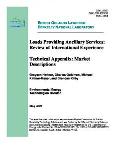
Fig. 1: Water inflows for a storage power plant in the Swiss Alps for some years to illustrate the strong seasonality.
The optimization is done for a typical Swiss storage power plant with a large hydro head and high power / storage ratio. The water levels in the basins have negligible influence on the production and it can be assumed that the power plant is operated as peak power plant. Therefore startup costs, water flow and dynamics, as well as non-linear, non-convex efficiency factors, can be neglected without loss of accuracy. The considered power plant is structured in such a way that it can be aggregated into an upper and lower basin with the ability to produce electricity as well as to pump water from the lower basin to the upper. The water inflows originate mostly from glacierized catchment in the Swiss Alps. Therefore a strong seasonality in inflows is present, and it is common to have a fully depleted upper basin in late-winter (see also Fig. 1). Because of the strong seasonality and capability to deplete the upper basin fast, the water has high opportunity costs. Therefore the decision of how much power to offer as secondary control influences
2
the estimation of the water values particularly. Proposed is a two-stage2 stochastic program to model the problem. In the first stage the algorithm has to decide on the amount of secondary control to offer for the next time period (a week) and a fixed price. At that moment, the algorithm knows nothing about the actual occurring electricity market prices. In the second stage the algorithm optimally produce electricity and pump, using the then known prices. This recourse action is modeled as a linear program, consisting of hourly stages for one week with different price scenarios. The overall optimization is solved by a stochastic dynamic programming (SDP) approach. The time horizon is at most one year with weekly time steps, starting at the beginning of snow and ice smelt in May. The basins are empty at the beginning. In real operation the algorithm would be applied with a receding horizon. In the case study the methodology is applied to a typical Swiss hydro plant. It will be shown, how such an optimization could act as a decision support for production particularly regarding offering of secondary control. In a forward simulation the methodology is tested on a realistic scenario. For an overview of stochastic programming in the energy sector [2] can be recommended. For SDP in hydro power planning see e.g. [3], for a review [4]. A survey about ancillary services in various parts of the world (but not Switzerland) can be found here [1]. Ancillary services were mostly considered in bidding problems. In [5] a decision support tool for market players is presented, by a deterministic multi-agent based simulator taking into account ancillary services. In [6] and [7] deterministic mixed-integer (non)-linear programs are presented to solve the bidding problem for a hydro power producer also with considering ancillary services. [8–10] use stochastic mixed-integer programming to account for uncertainties in electricity market and ancillary services market for a more short-term risk constrained scheduling optimization. In [11] the bidding and scheduling problem is optimized for an 11-unit system by a stochastic mixed-integer optimization, solved by an algorithm based on Lagrangian relaxation and SDP. This paper is organized as follows: Section 2 explains the model and its characteristics, mathematical representation and some computational remarks are given. Section 3 reveal the case study and finally section 4 concludes the paper.
2. The Model Table I: Explanation of the variables
Variable
t x
θ t,x
bidt,x
cbidt
Explanation Stage Discrete basin filling (state variable) [MWh] Profit-to-go [€] Discretized size of secondary control capacity block [MW] Estimated demand charge for secondary control bid [€/MW/h]
binbidt,x τ
Binary Variable: 0 if secondary control is offered, 1 otherwise
cpoolτ ,t
Estimated pool price [€/MWh]
Hourly stages within second stage
2
In this paper the term stage is used for denoting both optimization level and time point. There will be no explicit distinction made. However the meaning should be clear in the context.
3
hpdτ ,t,x hudτ ,t,x
Hourly decision of electricity production [MWh] Hourly usage of electricity (for pumping) decision [MWh]
efft
Efficiency of turbine
effp
Efficiency of pump
Ft,x
Valuing function for second stage
techmin
Minimum production amount [MW]
sd up t,x
Weekly spill decision for upper basin [MWh]
hsd τlow ,t,x turbτ ,t,x
inflt dur
p1, p2
Hourly spill decision for lower basin [MWh] Discretized amount of available water to discharge [MWh] Deterministic water inflows [MWh] Time duration of one stage t (one week) in hours [h] Penalty factors for spill in objective function [€/MWh]
In Switzerland and many other countries with deregulated electricity markets, a generation company is allowed to provide secondary control after a positive prequalification. After that bids for secondary control can be submitted to the Swiss TSO swissgrid, where the bids are accepted or not depending on a cost minimization algorithm. The bids have to be specified by both capacity block and demand charge. The capacity block has to be symmetric and at minimum ±5 MW with increments of at least 1 MW. This capacity has to be provided for the duration of the entire tender period (at the moment one week). Delivered energy is remunerated based on the pool prices for electricity. It is assumed, that all bids will get accepted so the power plant is a price-taker. It is also assumed, that requested energy from the TSO out of secondary control is symmetric. Further the remuneration of this energy is also neglected.
Fig. 2: Segmented power range of a pumped hydro power plant.
Fig. 2 shows the segmented power range of a Swiss storage hydro power plant. Since also the negativ part of the offered secondary control has to be delivered at any time, the turbines have to continously running at that amount of power. To prevent, that the turbines are operated unefficiently, a technical minimum is introduced. Further, for the power plant in the case study, pumping is not meaningful if secondary control is offered because of technical reasons. So the offering of secondary control reduces the production flexibility considerably.
4
2nd week
secondary contr.
1st week
secondary contr.
here-and-now decisions (weekly)
t 00 01 02
00
wait-and-see decisions (hourly) Fig. 3: Two-stage stochastic program with weekly decisions about secondary control and hourly recourse actions.
As already mentioned in the introduction, a two-stage stochastic program is proposed (see also Fig. 3). In the first stage the so called here-and-now decision has to be taken, where the algorithm has to decide on the amount of secondary control to offer without knowing the actual pool prices. The second stage is also known as recourse action, where the algorithm can react on the then known pool prices by adjusting its production, which is often expressed as wait-and-see decisions. The second stage is modeled as a linear program. Uncertainty to the accepted demand charge for secondary control bid as well as to the pool prices is introduced via scenarios.
Fig. 4: Discretization of the state and decision variables, the basin filling and the water used for generation. The problem reduces to a shortest path problem, which can be solved recursively.
Because the cumulated profit of a power plant is strictly increasing in time, a decomposition is meaningful. By also discretizing the state and decision space (see Fig. 4) the well known SDP scheme is attained (introduced in [12] and [13], first applied to hydro power planning problems in [14]). So for all possible basin levels, the most profitable case is recursively searched for, which is similar to a shortest path problem. The model is applied to a storage hydro power plant which can be aggregated into two basins. The upper basin act as monthly and seasonal storage whereas the lower one provides daily and hourly water to pump. So the water balance of the upper basins is done weekly for stages t, whereas for the lower one it is done hourly for stages τ .
2.1. Mathematical model Let θ t,x be the future expected profit for a state x at time t , also denoted profit-to-go. Then this profit-
to-go can be recursively calculated:
⎧ ⎫ θ t,x = max ⎨ E ⎡⎢ bidt,x ⋅ cbidt ⋅ dur + E ⎡⎣ Ft,x + θ t+1,x ⎤⎦ ⎤⎥ ⎬ cbidt ⎣ cpoolt ⎦⎭ ⎩
(1)
with E , E being the expected value over all secondary control demand charges and pool price cbidt cpoolt
scenarios respectively. Ft,x itself is a deterministic maximization problem depending on time, state and pool price scenario.
5
For each price scenario Ft,x can be stated as:
{
up Ft,x = max ( hpdτ ,t,x − hudτ ,t,x ) ⋅ cpoolτ ,t − sdt,x ⋅ p1 − hsd τlow ,t,x ⋅ p2
}
(2.1)
subject to the following equality constraints:
∑ (hpd τ
τ ,t,x
)
/ efft − hudτ ,t,x ⋅ effp + sd up t,x = turbt,x + inflt − binbidt,x ⋅ ( bidt,x + techmin ) ⋅ dur / efft
(2.2)
low low basinτlow ,t,x − basinτ −1,t,x − hpdτ ,t,x / efft + hudτ ,t,x ⋅ effp + hsd τ ,t,x =
binbidt,x ⋅ ( bidt,x + techmin ) / efft
∀τ
(2.3)
∀τ
(2.4)
∀τ
(2.5)
and bounds to the variable spaces:
0, techmin ≤ hpdτ ,t,x ≤ hpdmax − binbidt,x ⋅(2 ⋅ bidt,x + techmin) 0 ≤ hudτ ,t,x ≤ hudmax − binbidt,x ⋅(hudmax )
0 ≤ sd up t,x ≤ ∞
(2.6)
low 0 ≤ basinτlow ,t,x ≤ basin max
∀τ
(2.7)
0 ≤ hsd τlow ,t,x ≤ ∞
∀τ
(2.8)
The positive factors p1, p2 in equation 2.1 make sure, that, together with equation 2.3 and the variable bounds, the correct water balance in the lower basin is achieved. These factors can also be chosen as penalty for spill. Otherwise equation 1 has to be slightly modified to account for the correct profit obtained within the second stage. The discretized amount of available water to discharge turbt,x depends on the basin level and time stage in order to be meaningful. The algorithm tries to deploy this available water most profitable among the hourly stages τ within the second stage by producing or using power for pumping. Pumping is only allowed if no secondary control is offered. Problem (2.1) is a mixed-integer linear problem for τ stages and bidt,x as integer, binbidt,x as binary
up and hpdτ ,t,x , hudτ ,t,x , hsd τlow ,t,x , sdt,x as continuous variables. This problem can be efficiently solved since the amount of stages τ is limited.
Ft,x is calculated for every pool price scenario, which together with its probability, yield to the profitto-go. Similarly this is repeated for all basin levels and demand charges for secondary control, in order to calculate the expected profit over all demand charges (equation 1). The whole procedure is recursively done for all time stages until the first stage is reached. Out of the profit-to-go function for the first stage θ1,x , the water values can be constructed through its derivative.
2.2. Computational remarks All optimizations were done in Matlab R2011b with the standard optimization toolbox. The stochastic dynamic program problem can be formulated embarrassingly parallel, so that the optimizations took no longer than 20 minutes with a standard computer, with a quad-core 2.3 GHz Intel Core i7 processor and 8 GB of RAM. 6
However, if the special structure of the dynamic program is not exploited in the algorithm, it can easily take hours to solve. Effective actions for optimizing the algorithm are for instances to make sure, that the number of steps for the basin discretization is a multiple of the available computing units and that the work can be equally distributed across these units.
3. Case Study The model is applied to a Swiss hydro storage power plant. Installed production capacity is 240 MW with 200 GWh of storage in the upper basin. There is at maximum 40 MW of secondary control possible because of the internal structure of the power plant. The technical production minimum is 26 MW (see also Fig. 2). The optimization starts at the beginning of snow melt in late-winter and ends one year after. Hydro inflows are deterministically estimated out of 6 years of historic data. Pool (hourly) and secondary control prices (the same for all stages, see also Fig. 5) are also estimated out of historic data. 0.4
0.35
0.3
probability
0.25
0.2
0.15
0.1
0.05
0 20
22
24
26
28
30
32
34
36
demand charge for secondary control € /MW/h
38
40
Fig. 5: Modeled demand charges for secondary control together with estimated probability.
Until the beginning of a week is reached, the stages are daily without the possibility to offer secondary control. After that, weekly time stages occur, with first two pool price scenarios and, in the second half of the year, with three scenarios. For all stages there are five different possible accepted demand charges for secondary control (Fig. 5). There are 12 discretization steps for the basin and 8 for the offer of secondary control. water value [ € /MWh]
profit-to-go [relative]
70
1 0.8 0.6 0.4 0.2 0 0
0 2
10
4
20
stage
6
30 8
40 50
10 60
12
basin level
60 50 40 30 20 10 0 1
2
3
4
5
basin level
6
7
8
9
10
11
12
Fig. 6: Profit-to-go for all basin levels and stages and its derivative for the first stage, the water value for all basin levels.
Fig. 6 on the left shows the profit-to-go function for all basin levels and time stages. One recognizes the concavity of the profit-to-go within each stage as well as the strictly increasing profit with more stages. Also mentionable are the winter months (around stage 40), where because of essentially zero water inflows the profit-to-go does not change much. Fig. 6 on the right shows the derivation of the profit-to-go function for the first stage θ1,x , the water values for all basin levels. This is one of the main outputs of the simulation. If the basin is full, the water is roughly half of the value than if the basin is empty. Traders can use these values directly as decision support in their daily business.
7
Fig. 7 on the left shows the optimal offered capacity blocks of secondary control, which is the second main output of the optimization. The fuller the basin or the higher the expected pool prices, the more generation and by that also offering of secondary control may be more probable. However, with the provision of secondary control, the production flexibility is reduced because no pumping and less maximum generation are possible. So it may get also unprofitable with fuller basins, as clearly visible in the first stage, because the maximal generation capability is not available. Generation [MW] (MW) Offered secondary Control [MW] (MW) Pumping [MW] (MW) Pool price [Euro/MWh] (Euro/MWh)
35
200
30 25 20
150
15 10
MW
capacity blocks [MW]
40
5 0
100
0 10
50
20 30
stage
40 50 60
1
4
8
0 7650
12
7700
7750
7800
7850
7900
7950
8000
time [h]
basin level
Fig. 7: Optimal offered capacity blocks of secondary control for all stages and basin levels and detailed look in the simulation.
2.5 2 1.5 1 0.5 0 0
0 2 10
4 20
stage
6 30
40
8 50
10 60
12
basin level
profit-to-go difference (%)
profit-to-go difference (%)
On the right hand side of Fig. 7 a detailed look in the optimization is revealed, to illustrate what the algorithm is actually doing. For a fixed basin state two weeks are shown. One possible scenario of the pool price is depicted. The algorithm tries to deploy the available water most profitable within a week (where the prices are known in advance), which means generation at high prices and pumping in the lower ones. In the second week shown here, the pool prices are on average a bid higher, that’s why offering of secondary control may have got beneficial.
25 20 15 10 5 0 0
10
20
stage
30
40
50
60
12
10
8
6
4
2
0
basin level
Fig. 8: Profit-to-go differences in simulations: Left: Optimal solution vs. solution without possibility to offer secondary control. Right: Solution without secondary control vs. solution with always offering maximal secondary control bid.
Fig. 8 shows on the left a comparison for optimizations regarding the possibility to offer secondary control and without it. The difference is quite small (1-2% more profit if secondary control is considered) and therefore not really expressive. One could argue that the offering of secondary control doesn’t influence the profit at all. However, on the right of Fig. 8 is a comparison of an optimization without secondary control and an optimization where secondary control is offered every week. Here the profit, where secondary control is always offered, is around 15-25% lower. So these results would suggest for this case study, that if one wants to take the opportunity to also offer secondary control, one has to do that wisely. In order to clarify further the benefit of considering secondary control in the optimization a simulation was done on how such an optimization could be applied in reality. The simulation starts with empty 8
basins in late spring and then decides hourly of its generation by comparing the water value (together with turbine and pump efficiencies) with the pool price. It is important to note, that the simulation decides hourly without any idea of future prices. The basins are then hourly updated. The water value is interpolated out of the updated upper basin filling and the weekly water values of the medium-term optimization. For the sake of simplicity, the medium-term optimization is done only once. So it is assumed, that no additional information get available. Pool prices are taken from a historic year, which is not considered in the optimization.
Fig. 9: Forward simulation where the proposed optimization provides optimal secondary control bids and water values.
Fig. 9 shows the result of this forward simulation. As expected, the upper basin stores the water inflows in order to be able to generate power in the autumn and winter period. However, because the prices are relatively high in the summer (and the water value low), there is a lot of generation earlier, so that the upper basin is not fully filled. The lower basin is not shown here, because it fluctuates too much and only influences the pumping capability. Secondary control is offered nowhere. The reason for that could be the relatively low basin filling (see also Fig. 7 with the optimal secondary control bids). The profit out of this forward simulation results to 22.7 millions of Euro. The same forward simulation, but taking as guidelines the results from a medium-term optimization without considering secondary control, leads to a profit of 22.5 millions of Euro. This small difference in profits is also expected since secondary control is not beneficial for this case. A comparison with Fig. 7 shows the completely different behavior of optimal generation because of different pool prices. This can be seen as one motivation to use stochastic programming.
4. Conclusion In this paper a methodology is proposed, to include the ability to offer secondary control in a seasonal medium-term self-scheduling of a price-taker hydro power producer with pumped storage. The resulting linear mixed-integer problem is solved by a stochastic dynamic programming scheme. The second stage is modelled itself as a mixed-integer linear program, which makes it easily possible to account for different constraints. The methodology was applied to a Swiss hydro power plant and also tested in a forward simulation. The results suggest, that offering of secondary control could be beneficial. However, at the current accepted demand charges, one has to carefully decide at which point to do it. The proposed algorithm could help with this decision. It should be also noted, that the results heavily depend on the estimation of the pool prices. Whereas the stochastic modelling helps to make the optimization robust, additional risk constraints would be meaningful and is point of current work.
9
5. Acknowledgment The authors would like to thank EGL AG to provide power plant data and valuable support as well as KTI (Swiss Innovation Promotion Agency), project 11635.2, for financial support. BIBLIOGRAPHY [1] Y.G. Rebours, D.S. Kirschen, M. Trotignon, and S. Rossignol, “A survey of frequency and voltage control ancillary services: Part I & II”, IEEE Transactions on Power Systems, vol. 22, no 1, February 2007, pp. 358-366. [2] S.W. Wallace and S-E. Fleten, “Stochastic programming models in energy”, Stochastic Programming in Handbooks in Operations Research and Management Science, vol.10, Elsevier, 2003, pp. 637 – 677. [3] O. Fosso, A. Gjelsvik, A. Haugstad, B. Mo, and I. Wangensteen, “Generation scheduling in a deregulated system: The norwegian case”, IEEE Transactions on Power Systems, vol. 14, no. 1, February 1999, pp. 75 –81. [4] J. W. Labadie, “Optimal operation of multireservoir systems: State-of-the-art review”, Journal of Water Resources Planning and Management, vol. 130, no. 2, March 2004, pp. 93–111. [5] Z.A. Vale, C. Ramos, P. Faria, J.P. Soares, B. Canizes and H.M. Khodr, “Ancillary services dispatch using Linear Programming and Genetic Algorithm approaches”, MELECON 2010 - 2010 15th IEEE Mediterranean Electrotechnical Conference, April 2010, pp. 667 -672. [6] B. Zvonko, “Three utilization patterns of the renovated Moste hydro power plant on an electricity market of power and ancillary services”, Electric Power Systems Research, vol. 77, no. 34, 2007, pp. 252 - 258. [7] S.J. Kazempour, M. Hosseinpour and M.P. Moghaddam, “Self-scheduling of a joint hydro and pumped-storage plants in energy, spinning reserve and regulation markets”, IEEE Power Energy Society General Meeting, 2009, July 2009, pp. 1 -8. [8] S.-J. Deng, Y. Shen and H. Sun, “Optimal Scheduling of Hydro-Electric Power Generation with Simultaneous Participation in Multiple Markets”, IEEE Power Systems Conference and Exposition PSCE 2006, November 2006, pp. 1650 -1657. [9] L. Wu, M. Shahidehpour and Z. Li, “GENCO's Risk-Constrained Hydrothermal Scheduling”, vol. 23, no. 4, November 2008, pp. 1847 -1858. [10] A. Ugedo and E. Lobato, “Validation of a strategic bidding model within the Spanish sequential electricity market”, IEEE 11th International Conference on Probabilistic Methods Applied to Power Systems (PMAPS), June 2010, pp. 396 -401. [11] E. Ni and P.B. Luh, “Optimal integrated generation bidding and scheduling with risk management under a deregulated daily power market”, IEEE Power Engineering Society Winter Meeting, vol. 1, 2002, pp. 70 - 76. [12] P. Masse, Les Reserves et la Regulation de l’Avenir, Paris: Hermann, 1946. [13] R. Bellman, Dynamic Programming, New Jersey: Princeton University Press, 1957. [14] J.D.C. Little, “The use of storage water in a hydroelectric system”, Journal of the Operations Research Society of America, vol. 3, no. 2, 1955, pp. 187–197.
10