Approximability of the Minimum Weighted Doubly Resolving Set ...

Approximability of the Minimum Weighted Doubly Resolving Set Problem ∗

arXiv:1404.4676v1 [cs.DM] 18 Apr 2014

Xujin Chen

Xiaodong Hu

Changjun Wang

Academy of Mathematics and Systems Science Chinese Academy of Sciences, Beijing 100190, China {xchen,xdhu,wcj}@amss.ac.cn

Abstract Locating source of diffusion in networks is crucial for controlling and preventing epidemic risks. It has been studied under various probabilistic models. In this paper, we study source location from a deterministic point of view by modeling it as the minimum weighted doubly resolving set (DRS) problem, which is a strengthening of the well-known metric dimension problem. Let G be a vertex weighted undirected graph on n vertices. A vertex subset S of G is DRS of G if for every pair of vertices u, v in G, there exist x, y ∈ S such that the difference of distances (in terms of number of edges) between u and x, y is not equal to the difference of distances between v and x, y. The minimum weighted DRS problem consists of finding a DRS in G with minimum total weight. We establish Θ(ln n) approximability of the minimum DRS problem on general graphs for both weighted and unweighted versions. This is the first work providing explicit approximation lower and upper bounds for minimum (weighted) DRS problem, which are nearly tight. Moreover, we design first known strongly polynomial time algorithms for the minimum weighted DRS problem on general wheels and trees with additional constant k ≥ 0 edges.

Keywords: Source location, Doubly resolving set, Approximation algorithms, Polynomial-time solvability, Metric dimension

1

Introduction

Locating the source of a diffusion in complex networks is an intriguing challenge, and finds diverse applications in controlling and preventing network epidemic risks [17]. In particular, it is often financially and technically impossible to observe the state of all vertices in a large-scale network, and, on the other hand, it is desirable to find the location of the source (who initiates the diffusion) from measurements collected by sparsely placed observers [16]. Placing an observer at vertex v incurs a cost, and the observer with a clock can record the time at which the state of v is changed (e.g., knowing a rumor, being infected or contaminated). Typically, the time when the single source originates an information is unknown [16]. The observers can only report the times they receive the information, but the senders of the information (i.e., we do not know who infects whom or who influences whom) [8]. The information is diffused from the source to any vertex through shortest paths in the network, i.e., as soon as a vertex receives the information, it sends the information to all its neighbors simultaneously, which takes one time unit. Our goal is to select a subset S of vertices with minimum total cost such that the source can be uniquely located by the “infected” times of vertices in S. This problem is equivalent to finding a minimum weighted doubly resolving set (DRS) in networks defined as follows. ∗ Research supported in part by NNSF of China under Grant No. 11222109, 11021161 and 10928102, by 973 Project of China under Grant No. 2011CB80800, and by CAS Program for Cross & Cooperative Team of Science & Technology Innovation.

1

DRS model. Networks are modeled as undirected connected graphs without parallel edges nor loops. Let G = (V, E) be a graph on n ≥ 2 vertices, and each vertex v ∈ V has aP nonnegative weight w(v), representing its cost. For any S ⊆ V , the weight of S is defined to be w(S) := v∈S w(v). For any u, v ∈ V , we use dG (u, v) to denote the distance between u and v in G, i.e., the number of edges in a shortest path between u and v. Let u, v, x, y be four distinct vertices of G. Following C´aceres et al. [2], we say that {u, v} doubly resolves {x, y}, or {u, v} doubly resolves x and y, if dG (u, x) − dG (u, y) 6= dG (v, x) − dG (v, y). Clearly {u, v} doubly resolves {x, y} if and only if {x, y} doubly resolves {u, v}. For any subsets S, T of vertices, S doubly resolves T if every pair of vertices in T is doubly resolved by some pair of vertices in S. In particular, S is called a doubly resolving set (DRS) of G if S doubly resolves V . Trivially, V is a DRS of G. The minimum weighted doubly resolving set (MWDRS) problem is to find a DRS of G that has a minimum weight (i.e. a minimum weighted DRS of G). In the special case where all vertex weights are equal to 1, the problem is referred to as the minimum doubly resolving set (MDRS) problem [15], and it concerns with the minimum cardinality dr(G) of DRS of G. Consider arbitrary S ⊆ V . It is easy to see that S fails to locate the diffusion source in G at some case if and only if there exist distinct vertices u, v ∈ V such that S cannot distinguish between the case of u being the source and that of v being the source, i.e., dG (u, x) − dG (u, y) = dG (v, x) − dG (v, y) for any x, y ∈ S; equivalently, S is not a DRS of G. (See Appendix A.) Hence, the MWDRS problem models exactly the problem of finding cost-effective observer placements for locating source, as mentioned in our opening paragraph. Related work. Epidemic diffusion and information cascade in networks has been extensively studied for decades in efforts to understand the diffusion dynamics and its dependence on various factors, such as network structures and infection rates. However, the inverse problem of inferring the source of diffusion based on limited observations is far less studied, and was first tackled by Shah and Zaman [17] for identifying the source of rumor, where the rumor flows on edges according to independent exponentially distributed random times. A maximum likelihood (ML) estimator was proposed for maximizing the correct localizing probability, and the notion of rumor-centrality was developed for approximately tracing back the source from the configuration of infected vertices at a given moment. The accuracy of estimations heavily depended on the structural properties of the networks. Shah and Zaman’s model and their results on trees were extended by Karamchandani and Franceschetti [11] to the case in which nodes reveal whether they have heard the rumor with independent probabilities. Along a different line, Pinto et al. [16] proposed other ML estimators that perform source detection via sparsely distributed observers who measure from which neighbors and at what time they received the information. The ML estimators were shown to be optimal for trees, and suboptimal for general networks under the assumption that the propagation delays associated with edges are i.i.d. random variables with known Gaussian distribution. In contrast to previous probabilistic model for estimating the location of the source, we study the problem from a combinatorial optimization’s point of view; our goal is to find an observer set of minimum cost that guarantees deterministic determination of the accurate location of the source, i.e., to find a minimum weighted DRS. The double resolvability is a strengthening of the well-studied resolvability, where a vertex x resolves two vertices u, v if and only if dG (u, x) 6= dG (v, x). A subset S of V is a resolving set (RS) of G if every pair of vertices is resolved by some vertex of S. The minimum cardinality of a RS of G is known as the metric dimension md(G) of G, which has been extensively studied due to its theoretical importance and diverse applications (see e.g., [2, 4, 7, 9] and references therein). Most literature on finding minimum resolving sets, known as the metric dimension problem, considered the unweighted case. The unweighted problem is N P hard even for planar graphs, split graphs, bipartite graphs and bounded degree graphs [6, 7, 9]. On general graphs, Hauptmann et al. [9] showed that the unweighted problem is not approximable within (1 − ε) ln n for any ε > 0, unless N P ⊂ DT IM E(nlog log n ); moreover, the authors [9] gave a (1 + o(1)) ln n-approximation algorithm based on approximability results of the test set problem in bioinformatics [1]. A lot of research efforts have been devoted to obtaining the exact values or upper bounds of the metric dimensions of special 2

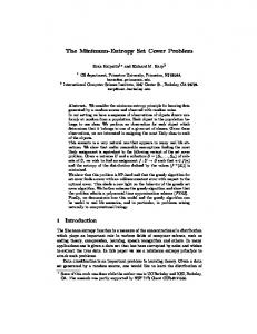
graphic classes [2]. Recently, Epstein et al [7] studied the weighted version of the problem, and developed polynomial time exact algorithms for finding a minimum weighted RS, when the underlying graph G is a cograph, a k-edge-augmented tree (a tree with additional k edges) for constant k ≥ 0, or a (un)complete wheel. Compared with nearly four decade research and vast literatures on resolving sets (metric dimension), the study on DRS has a relatively short history and its results have been very limited. The concept of DRS was introduced in 2007 by C´ aceres et al. [2], who proved that the minimum RS of the Cartesian product of graphs is tied in a strong sense to minimum DRS of the graphs: the metric dimension of the Cartesian product of graphs G1 and G2 is upper bounded by md(G1 ) + dr(G2 ). When restricted to the same graph, it is easy to see that a DRS must be a RS, but the reverse is not necessarily true. Thus md(G) ≤ dr(G). The ratio dr(G)/md(G) can be arbitrarily large. This can be seen from the tree graph G depicted in Fig. 1. On the one hand, it is easily checked that {r1 , r2 } is a RS of G, giving dr(G) ≤ 2. On the other hand, md(G) = n/2 since {s1 , s2 , . . . , sh } is the unique minimum DRS of G, as proved later in Lemma 4.1 of this paper. In view of the large gap, algorithmic study on DRS deserves good efforts, and it is interesting to explore the algorithmic relation between the minimum (weighted) DRS problem and its resolving set counterpart.

Figure 1: The graph tree G with dr(G) = n/2 and md(G) = 2. Previous research on DRS considered only the unweighted case. As far as general graphs are concerned, the MDRS problem has been proved to be N P -hard [14], and solved experimentally by metaheuristic approaches that use binary encoding and standard genetic operators [14] and that use variable neighborhood search [15]. To date, no efficient general-purpose algorithms with theoretically provable performance guarantees have been developed for the MDRS problem, let alone the MWDRS problem. Despite the NP-hardness, the approximability status of either problem has been unknown in literature. For special graphs, it is known ˇ that every RS of Hamming graph is also a DRS [12]. Recently, Cangalovi´ c et al. showed that dr(G) ∈ {3, 4} when G is a prism graph [3] or belongs to one of two classes of convex polytopes [13]. Our contributions. As far as we know, our opening example of cost-effective source location is the first real-world application of DRS explicitly addressed. Motivated by the application, we study and provide a thorough treatment of the MWDRS problem in terms of algorithmic approximability. Broadly speaking, we show that the MDRS and MWDRS problems have similar approximability to their resolving set counterparts. Based on the construction of Hauptmann et al. [9], we prove that there is an approximation preserving reduction from the minimum dominating set problem to the MDRS problem, showing that the MDRS problem does not admit (1 − ε) ln n-approximation algorithm for any ε > 0 unless N P ⊂ DT IM E(nlog log n ). The strong inapproximability improves the N P -completeness established in [14]. Besides, we develop a (ln n + ln log2 n + 1)-approximation algorithm for solving the MWDRS problem in O(n4 ) time, based on a modified version of the approximation algorithms used in [1, 9]. To the best of our knowledge, this paper is the first work providing explicit approximation lower and upper bounds for the MDRS and MWDRS problems, which are nearly tight (for large n). A byproduct of our algorithm gives the first logarithmic approximation for the weighted metric dimension problem on general graphs. Despite many significant technical differences between handling DRS and RS, we establish the polynomial time solvability of the MWDRS problem for all these graph classes, with one exception of cographs, where the weighted metric dimension problem is known to admit efficient exact algorithms [7]. Our results are first known strong polynomial time algorithms for the MDRS problem on k-edge-augmented trees and general wheels, including paths, trees and cycles. Using the fact that every minimum weighted DRS is minimal (with respect to the inclusion relation), our algorithms make use of the graphic properties to cleverly “enumerate” minimal doubly resolving sets that are potentially minimum weighted, and select the best one among them. 3

The paper is organized as follows: The inapproximability is proved in Section 2, The approximation algorithm for general graphs and exact algorithms for special graphs are presented in Sections 3 and 4, respectively. Future research directions are discussed in Section 5. The omitted details are given in Appendix.

2

Approximation lower bound

In this section, we establish a logarithmic lower bound for approximation the MDRS problem under the assumption that N P 6⊂ DT IM E(nlog log n ). Hauptmann et al. [9] constructed a reduction from the minimum dominating set (MDS) problem to the metric dimension problem. Although their proof does not work for DRS, we show that their construction actually provides an approximation preserving reduction from the MDS problem to the MDRS problem. A vertex subset S of graph G is a dominating set of G if every vertex outside S has a neighbor in S. The MDS problem is to find a dominating set of G that has the minimum cardinality ds(G). Unless N P ⊂ DT IM E(nlog log n ), the MDS problem cannot be approximated within (1 − ε) ln n for any ε > 0 [5]. Lemma 2.1. There exists a polynomial time transformation that transfers graph G = (V, E) to graph G′ = (V ′ , E ′ ) such that dr(G′ ) ≤ ds(G) + ⌈log2 n⌉ + 3. Let graphs G and G′ be as in Lemma 2.1. It has been shown that, given any RS (in particular DRS) S of G′ , a dominating set of G with cardinality at most |S| can be found in polynomial time [9]. This, in combination with Lemma 2.1 and the logarithmic inapproximability of the MDS problem [5], gives the following lower bound for approximating minimum DRS. Theorem 2.2. Unless N P ⊂ DT IM E(nlog(log n) ), the MDRS problem cannot be approximated in polynomial time within a factor of (1 − ǫ) ln n, for any ǫ > 0.

3

Approximation algorithm

In this section, we present an O(n4 ) time approximation algorithm for the MWDRS problem in general graphs that achieves approximation ratio (1 + o(1)) ln n, nearly matching the lower bound ln n established in Theorem 2.2. Our algorithm uses similar idea to that of Hauptmann et al. [9] for approximating minimum resolving sets in the metric dimension (MD) problem. The MD problem is a direct “projection” of the unweighted test set problem studied by Berman et al. [1] in the sense that a vertex in the MD problem can be seen as a “test” in the test set problem, which allows Hauptmann et al. to apply Berman-DasGupta-Kao algorithm [1] directly. However, in the DRS problem, one cannot simply view two vertices as a “test”, because such a “test” would fail the algorithm in some situation. Besides, the algorithm deals with only unweighted cases. Thus we need conduct certain transformation that transforms the DRS problem to a series of weighted test set problems. Furthermore, we need modify Berman-DasGupta-Kao algorithm to solve these weighted problems within logarithmic approximation ratios. Transformation. For any x ∈ V , let Ux = {{x, v} : v ∈ V \ {x}}. As seen later, each element of Ux can be viewed as a test or a certain combination of tests in the test set problem studied in [1]. From this point of view, we call each element of Ux a super test, and consider the minimum weighted super test set (MWSTS) problem on (V, Ux ) as follows: For each super test T = {x, v} ∈ Ux , let its weight be w(T ) = w(v), The problem is to find a set of super tests T ⊆ Ux such that each pair of vertices in G is doubly resolved by some P super test in T and the weight w(T ) = T ∈T w(T ) of T is minimized. The following lemma establishes the relation between the MWDRS problem and the MWSTS problem. Lemma 3.1. Let S be a DRS of G and s ∈ S. Then every pair of vertices in G is doubly resolved by at least one element of {{s, v} : v ∈ S \ {s}}.

4

Proof. Let u, v be any two distinct vertices of G. There exist s1 , s2 ∈ S such that dG (u, s1 ) − dG (v, s1 ) 6= dG (u, s2 ) − dG (v, s2 ). It follows that either dG (u, s1 ) − dG (v, s1 ) 6= dG (u, s) − dG (v, s) or dG (u, s) − dG (v, s) 6= dG (u, s2 ) − dG (v, s2 ), saying that u and v are doubly resolved by either {s, s1 } or {s, s2 }. Since V is a DRS of G, Lemma 3.1 implies that Ux doubly resolves V . More importantly, Lemma 3.1 provides the following immediate corollary that is crucial to our algorithm design. Corollary 3.2. Let S ∗ be a minimum weighted DRS of G and α ∈ S ∗ . Then the minimum weight of a solution to the MWSTS problem on (V, Uα ) is at most w(S ∗ ) − w(α). Approximation. In order to solve the MWSTS problem, we adapt Berman-DasGupta-Kao algorithm [1] to augment a set T (⊆ Ux ) of super tests to be a feasible solution step by step. We define equivalence relation ≡T on V by: two vertices u, v ∈ V are equivalent under ≡T if and only if {u, v} is not doubly resolved by any test of T . Clearly, the number of equivalence classes is non-decreasing with the size of T . Let E1 , . . . , Ek Q be the equivalence classes of ≡T . The value HT := log2 ( ki=1 |Ei |!) is called the entropy of T . Note that HT = 0

⇔ every equivalent class of ≡T is a singleton ⇔ ∪T ∈T T is a DRS of G.

(3.1)

Hence our task is reduced to finding a set T of super tests with zero entropy HT and weight w(T ) as small as possible. For any super test T ∈ Ux , an equivalence class of ≡T is either an equivalence class of ≡T ∪T or it is partitioned into several (possibly more than two) equivalence classes of ≡T ∪T . (If T partitions each equivalent class into at most two equivalent classes, then T works as a test in the test set problem.) Therefore HT ≥ HT ∪T , and IC(T, T ) := HT − HT ∪T ≥ 0 equals the decreasing amount of the entropy when adding T to T . It is clear that IC(T, ∅) ≤ log2 n! − log2 1 < n log2 n.

(3.2)

We now give a (1+o(1)) ln n-approximation algorithm for the MWSTS problem on (V, Ux ). The algorithm adopts the greedy heuristic to decrease the entropy of the current set of super tests at a minimum cost (weight). Algorithm 1. Finding minimum weighted set T of super sets. 1.

T ←∅

2.

while HT 6= 0 do

3.

Select a super test T ∈ Ux − T that maximizes

4.

T ←T ∪T

5.

IC(T,T ) w(T )

end-while

The major difference between Algorithm 1 and the algorithms in [1, 9] is the criterion used in Step 3 for selecting T . It generalizes the previous unweighted setting. The following lemma extends the result on test set [1] to super test set. Lemma 3.3. IC(T, T0 ) ≥ IC(T, T1 ) for any sets T0 and T1 of super tests with T0 ⊆ T1 . Using (3.2) and Lemma 3.3, the proof of performance ratio goes almost verbatim as the argument of Berman et al. [1]. We include a proof in Appendix C for completeness. Theorem 3.4. ÅAlgorithm 1 isãan O(n3 ) time algorithm for the MWSTS problem on (V, Ux ) with approximation ratio ln max IC(T, ∅) +1 ≤ ln n+ln log2 n+1.✷ T ∈Ux

Suppose that given the MWSTS problem on (V, Ux ), Algorithm 1 outputs a super test set Tx . By (3.1), Running Algorithm 1 for n times, we obtain n doubly resolving sets Sx , x ∈ V of G, from which we select the one, say Sv , that has the minimum weight, i.e. w(Sv ) = min{w(Sx ) : x ∈ V }. 5

Theorem 3.5. The MWDRS problem can be approximated in O(n4 ) time within a ratio Å ã ln max IC({u, v}, ∅) + 1 ≤ ln n + ln log2 n + 1 = (1 + o(1)) ln n. u,v∈V

Proof. Let S ∗ be an optimal solution to the MWDRS problem. It suffices to show w(Sv )/w(S ∗ ) ≤ (1 + o(1)) ln n. Take α ∈ S ∗ , and let Tα∗ be an optimal solution to the MWSTS problem on (V, Uα ). It follows from the choice of Sv , Theorem 3.4 and Corollary 3.2 that w(Sv ) ≤ w(Sα ) = w(α) + w(Tα ) ≤ w(α) + (ln n + ln log2 n + 1)w(Tα∗ ) < (ln n + ln log2 n + 1)w(S ∗ ). Our algorithm and analysis show that the algorithm of [1] can be extended to solve the weighted test set problem, where each test has a nonnegative weight, by changing the selection criterion to be maximizing IC(T, T ) divided by the weight of T . A similar extension applied to the algorithm of Hauptmann et al. [9] gives a (1 + o(1)) ln n-approximate solution to the weighted metric dimension problem.

4

Exact algorithms

Let k ≥ 0 be a constant. A connected graph is called a k-edge-augmented tree if the removal of at most k edges from the graph leaves a spanning tree. Trees and cycles are 0-edge- and 1-edge-augmented trees, respectively. We design efficient algorithms for solving the MWDRS problem exactly on k-edge-augmented trees. Our algorithms run in linear time for k = 0, 1, and in O(n12k ) time for k ≥ 2. A graph is called a general wheel if it is formed from a cycle by adding a vertex and joining it to some (not necessarily all) vertices on the cycle. We solve the MWDRS problem on general wheels in cubic time by dynamic programming.

4.1

k-edge-augmented trees

Let G = (V, E) be a k-edge-augmented tree, and let L be the set of leaves (degree 1 vertices) in G. For simplicity, we often use d(u, v) instead of dG (u, v) to denote the distance between vertices u, v ∈ V in the underlying graph G of the MWDRS problem. 4.1.1

Trees: the case of k = 0.

When k = 0, graph G = (V, E) is a tree. There is a fundamental difference between DRS and RS of G in terms of minimal sets. In general, G may have multiple minimal RSs and even multiple minimum weighted RSs. Nevertheless, in any case G has only one minimal DRS, which consists of all its leaves. In particular, we have dr(G) = |L|. Lemma 4.1. L is the unique minimal DRS of G. Proof. For any two vertices u, v ∈ V , there exist leaves l1 , l2 ∈ L such that the path between l1 and l2 goes through u and v. It is easy to see that d(u, l1 ) − d(u, l2 ) 6= d(v, l1 ) − d(v, l2 ). So L is a DRS. On the other hand, consider any leaf l ∈ L and its neighbor p ∈ V . Since d(l, v) − d(p, v) = 1 for any v ∈ V − {l}, we see that each DRS of G contains l, and thus L. The conclusion follows. 4.1.2

Cycles: a special case of k = 1.

Let G = v1 v2 · · · vn v1 be a cycle, where V = {v1 , v2 , . . . , vn }. Suppose without loss of generality that w(vp ) = minni=1 w(vi ), where p := ⌈n/2⌉. It was known that any pair of vertices whose distance is not exactly n/2 is a minimal RS of G, and vice versa [7]. As the next lemma shows, the characterization of DRS turns out to be more complex. Each nonempty subset S of V cuts G into a set PS of edge-disjoint paths such that they are internally disjoint from S and their union is G. Lemma 4.2. Given a cycle G = (V, E), let S be a nonempty subset of V . Then S is a DRS of G if and only if no path in PS has length longer than ⌈n/2⌉ and at least one path in PS has length shorter than n/2. 6

An instant corollary reads: The size of a minimal DRS of cycle G is 2 or 3 when n is odd, and is 3 when n is even; In particular, dr(G) = 2 when n is odd, and dr(G) = 3 when n is even. These properties together with the next one lead to our algorithm for solving the MWDRS problem on cycles. Corollary 4.3. If some minimum weighted DRS has cardinality 3, then there exists a minimum weighted DRS of G that contains vertex vp . Algorithm 2. Finding minimum weighted DRS S in cycle G. 1. ω ← w(v1 ), i[1] ← 1, j ← 1, W ← w(V ) 2. for h = 1 to p do 3.

if w(vh ) < ω then j ← j + 1, i[j] ← h, ω ← w(vh )

4. end-for 5. if j > 1 then k ← j else k ← 2, i[k] ← p 6. if n is odd then S ← arg minn i=1 w({vi , vi+p−1 }), W ← w(S) 7. for j = 1 to k − 1 do i[j+1]+p

8.

let uj be a vertex in {vh : i[j] + p ≤ h ≤ i[j + 1] + p} with w(uj ) = minh=i[j]+p w(vh )

9.

if w(vp ) + w(vi[j] ) + w(uj ) < W then S ← {vp , vi[j] , uj }, W ← w(S)

10. end-for

Note that Vj := {vh : i[j] + p ≤ h ≤ i[j + 1] + p}, j = 1, . . . , k − 1 induce k − 1 internally disjoint paths in G. It is thus clear that Algorithm 2 runs in O(n) time. The vertices indices 1 = i[1] < i[2] < · · · < i[k] = p i[j+1]−1 i[j+1]−1 w(vh ) for every j = 1, . . . , k − 1 found by the algorithm satisfy w(vi[j] ) = minh=i[j] w(vh ) = minh=1 p and w(vi[k] ) = w(vp ) = minh=1 w(vh ). Moreover, either w(v1 ) = w(vp ) and k = 2, or w(vi[j] ) > w(vi[j+1] ) for every j = 1, . . . , k − 1. These facts together with the properties mentioned above verify the correctness of the algorithm. Theorem 4.4. Algorithm 2 finds in O(n) time a minimum weighted DRS of cycle G. 4.1.3

The case of general k.

Our approach resembles at a high level the one used by Epstein et al. [7]. However, double resolvablity imposes more strict restrictions, and requires extra care to overcome technical difficulties. Let Gb = (Vb , Eb ) be the graph obtained from G = (V, E) by repeatedly deleting leaves. We call Gb the base graph of G. We reduce the MWDRS problem on G to the MWDRS problem on Gb (see Lemma 4.5). The latter problem can be solved in polynomial time by exhaustive enumeration, since, as proved in the sequel, every minimal DRS of Gb has cardinality at most 12(k − 1) for k ≥ 2 Clearly, Gb is connected and has minimum degree at least 2. A vertex in Vb is called a root if in G it is adjacent to some vertex in V \ Vb . Let R denote the set of roots. Clearly, R ∩ L = ∅. In Gb , we change the weights of all roots to zero, while the weights of other vertices remain the same as in G. Lemma 4.5. Suppose that Sb is a minimum weighted DRS of Gb . Then (Sb \ R) ∪ L is a minimum weighted DRS of G. Therefore, for solving the MWDRS problem on a weighted k-edge-augmented tree G, we only need to find a minimum weighted DRS of base graph Gb with the weights of all roots modified to be 0. For 1-edge-augmented tree G, its base graph Gb is a cycle, whose minimum weighted DRS can be found in O(n) time (recall Algorithm 2). Combining this with Lemmas 4.1 and 4.5, we have the following linear time solvability. Theorem 4.6. There is an O(n) time exact algorithm for solving the MWDRS problem on k-edge-augmented trees, for k = 0, 1, including trees and cycles. 7

In the remaining discussion for k-edge-augmented tree, we assume k ≥ 2. A vertex is called a branching vertex of a graph if it has degree at least 3 in the graph. Recall that every vertex of the base graph Gb = (Vb , Eb ) has degree at least 2. It can be shown that (see Lemmas E.1 and E.2 in Appendix E) • In O(|Eb |) = O(n2 ) time, Gb can be decomposed into at most 3k − 3 edge-disjoint paths whose ends are branching vertices of Gb and internal vertices have degree 2 in Gb . • For any minimal DRS set S of Gb , and any path P in the above path decomposition of Gb , at most four vertices of S are contained in P . It follows that every minimal DRS of Gb contains at most 12(k − 1) vertices. Our algorithm for finding the minimum weighted DRS of Gb examines all possible subsets of Vb with cardinality at most 12(k − 1) by taking at most four vertices from each path in the path decomposition of Gb ; among these sets, the algorithm selects a DRS of Gb with minimum weight. Have a table that stores the distances between each pair of vertices in Gb , it takes O(n2 ) time to test the double resolvability of a set. Recalling Lemma 4.5, we obtain the following strong polynomial time solvability for the general k-edge-augmented trees. Theorem 4.7. The MWDRS problem on k-edge-augmented trees can be solved in O(n12k ) time.

4.2

Wheels

A general wheel G = (V, E) on n (≥ 6) vertices v1 , v2 , . . . , vn is formed by the hub vertex vn and a cycle C = (Vc , Ec ) over the vertices v1 , v2 , . . . , vn−1 , called rim vertices, where the hub is adjacent to some (not necessarily all) rim vertices. We develop dynamic programming algorithm to solve the MWDRS problem on general wheels in O(n3 ) time. We start with complete wheels whose DRS has a very nice characterization that is related to the consecutive one property. A general wheel is complete if its hub is adjacent to every rim vertex. The distance in G between any two vertices in G is either 1 or 2.

(4.1)

Lemma 4.8. Given a complete wheel G = (V, E), let S be a proper nonempty subset of V . Then S is a doubly resolving set if and only if S ∩ V (C) is a dominating set of C and any pair of rim vertices outside S has at least two neighbors in S ∩ V (C). Proof. If S ∩ V (C) is not a dominating set of C, then there exists a vertex vi ∈ V (C) − S such that vi is not adjacent to any vertex of S ∩ V (C). In this case, S cannot doubly resolve {vn , vi } because for any s1 , s2 ∈ S, d(s1 , vn ) − d(s1 , vi ) = −1 = d(s2 , vn ) − d(s2 , vi ). If S ∩V (C) is a dominating set of C but there exist two cycle vertices vi , vj ∈ V (C)−S such that vi , vj are uniquely dominated by the same cycle vertex v ∈ S, then for any two vertices s1 , s2 ∈ S, d(s1 , vi )−d(s1 , vj ) = 0 = d(s2 , vi ) − d(s2 , vj ), saying that S is not a doubly resolving set. Suppose that S satisfies the condition stated in the lemma. We prove that S can resolve every pair of vertices x, y in G. When one of x and y, say x, is a rim vertex in S, since n ≥ 6, there exists another rim vertex z ∈ S − {x} that is not adjacent to x. It follows from (4.1) that {x, y} is resolved by {x, z} as d(x, x) − d(x, z) = −2 < −1 ≤ d(y, x) − d(y, z). When both x and y are rim vertices outside S, there are two rim vertices x′ and y ′ in S dominating x and y, respectively. It follows that {x, y} is resolved by {x′ , y ′ }. When one of x and y, say x is the hub, we only need consider the case of y is a rim vertex outside S. Take rim vertices z, z ′ from S such that z dominates y and z ′ does not dominate y. It follows that {x, y} is resolved by {z, z ′} as d(x, z) − d(x, z ′ ) = 0 < −1 = d(y, z) − d(y, z ′ ). The characterization in Lemma 4.8 can be rephrased as follows: A subset S ⊆ V is a DRS of G if and only if every set of three consecutive vertices on C contains at least one vertex of S, and every set of five consecutive vertices on C contains at least two vertices of S. This enables us to formulate the MWDRS problem on a complete wheel as an integer programming with consecutive 1’s and circular 1’s constraints, which can be solved in O(n3 log2 n) time by Hochbaum and Levin’s algorithm [10]. (To the best of our knowledge, 8

there is no such a concise way to formulate the metric dimension problem on complete wheels as an integer programming with consecutive one matrix.) Moreover, it is not hard to see from the characterization that linear time efficiency can be achieved by dynamic programming approach. Furthermore, we elaborate on the idea to solve the MWDRS problem on more complex general wheels. Theorem 4.9. The MWDRS problem on complete wheels can be solved in O(n) time. The MWDRS problem on general wheels can be solved in O(n3 ) time.

5

Conclusion

In this paper, we have established Θ(ln n) approximability of the MDRS and MWDRS problems on general graphs. There is still a gap of 1 + ln log2 n hidden in the big theta (see Theorems 2.2 and 3.4). It deserves good research efforts to obtain even tighter upper bounds for the approximability. The k-edge-augmented trees, general wheels and cographs are known graph classes on which the weighted metric dimension problem is polynomial time solvable. In this paper, we have extended the polynomial time solvability to the MWDRS problem for the first two graph classes. It would be interesting to see whether the problem on cographs and other graphs also admits efficient algorithms.

References [1] Piotr Berman, Bhaskar DasGupta, and Ming-Yang Kao. Tight approximability results for test set problems in bioinformatics. J. Comput. Syst. Sci., 71(2):145–162, 2005. [2] Jos´e C´aceres, Carmen Hernando, Merc´e Mora, Ignacio M. Pelayo, Mar´ıa L. Puertas, Carlos Seara, and David R. Wood. On the metric dimension of cartesian products of graphs. SIAM J. Discrete Math., 21(2):423–441, 2007. ˇ [3] Mirjana Cangalovi´ c, Jozef Kratica, Vera Kovaˇcevi´c-Vujˇci´c, and Milica Stojanovi´c. Minimal doubly resolving sets of prism graphs. Optimization, (ahead-of-print):1–7, 2013. [4] Gary Chartrand and Ping Zhang. The theory and applications of resolvability in graphs: A survey. Congressus Numerantium, 160:47–68, 2003. [5] M. Chleb´ık and J. Chleb´ıkov´a. Approximation hardness of dominating set problems in bounded degree graphs. Inf. Comput., 206(11):1264–1275, 2008. [6] Josep D´ıaz, Olli Pottonen, Maria Serna, and Erik Jan van Leeuwen. On the complexity of metric dimension. In Algorithms–ESA 2012, pages 419–430. Springer, 2012. [7] Leah Epstein, Asaf Levin, and Gerhard J. Woeginger. The (weighted) metric dimension of graphs: hard and easy cases. In Proc. of the 38th international conference on Graph-Theoretic Concepts in Computer Science, WG’12, pages 114–125, 2012. [8] Manuel Gomez Rodriguez, Jure Leskovec, and Andreas Krause. Inferring networks of diffusion and influence. In Proc. of the 16th ACM SIGKDD international conference on Knowledge Discovery and Data mining, KDD ’10, pages 1019–1028, 2010. [9] Mathias Hauptmann, Richard Schmied, and Claus Viehmann. Approximation complexity of metric dimension problem. J. Discrete Algorithms, 14:214–222, 2012. [10] Dorit S Hochbaum and Asaf Levin. Optimizing over consecutive 1’s and circular 1’s constraints. SIAM J. Optimization, 17(2):311–330, 2006. [11] Nikhil Karamchandani and Massimo Franceschetti. Rumor source detection under probabilistic sampling. In Proc. of 2013 IEEE International Symposium on Information Theory, pages 2184–2188, 2013. 9

ˇ [12] Jozef Kratica, Vera Kovaˇcevi´c-Vujˇci´c, Mirjana Cangalovi´ c, and Milica Stojanovi´c. Minimal doubly resolving sets and the strong metric dimension of hamming graphs. Appl. Anal. Discret. Math., 6(1):63– 71, 2012. ˇ [13] Jozef Kratica, Vera Kovaˇcevi´c-Vujˇci´c, Mirjana Cangalovi´ c, and Milica Stojanovi´c. Minimal doubly resolving sets and the strong metric dimension of some convex polytopes. Appl. Math. Comput., 218(19):9790 – 9801, 2012. ˇ [14] Jozef Kratica, Mirjana Cangalovi´ c, and Vera Kovaˇcevi´c-Vujˇci´c. Computing minimal doubly resolving sets of graphs. Comput. Oper. Res., 36(7):2149–2159, 2009. ˇ [15] Nenad Mladenovi´c, Jozef Kratica, Vera Kovaˇcevi´c-Vujˇci´c, and Mirjana Cangalovi´ c. Variable neighborhood search for metric dimension and minimal doubly resolving set problems. Eur. J. Oper. Res., 220(2):328–337, 2012. [16] Pedro C. Pinto, Patrick Thiran, and Martin Vetterli. Locating the source of diffusion in large-scale networks. Phys. Rev. Lett., 109:068702, 2012. [17] Devavrat Shah and Tauhid Zaman. Rumors in a network: Who’s the culprit? IEEE Trans. Information Theory, 57(8):5163–5181, 2011.

Appendix A

Equivalence

We prove the equivalence between location sets and the doubly resolving sets in any graph G = (V, E). Observation 1. Let S ⊆ V . Then S fails to locate the diffusion source in G in some instance if and only if there exist distinct vertices u, v ∈ V such that S cannot distinguish between the case of u being the source and that of v being the source, i.e., dG (u, x) − dG (u, y) = dG (v, x) − dG (v, y) for any x, y ∈ S; equivalently, S is not a DRS of G. Proof. Consider distinct u, v ∈ V such that u or v is the information source. Let tx denote the time when x ∈ S receives the information. Suppose that dG (u, x) − dG (u, y) = dG (v, x) − dG (v, y) for any x, y ∈ S. Hence we have constant c such that dG (u, x) − dG (v, x) = c for any x ∈ S. It follows that the value of tx when u initiates the information at time 0 and that when v intimates the information at time c are the same, saying that S fails to be a location set. Suppose S is a DRS of G. So there exist x′ , y ′ ∈ S such that dG (u, x′ ) − dG (u, y ′ ) 6= dG (v, x′ ) − dG (v, y ′ ). If u is the source, then tx′ − ty′ = dG (u, x′ ) − dG (u, y ′ ); otherwise v is the source, and tx′ − ty′ = dG (v, x′ ) − dG (v, y ′ ). By checking the value tx′ − ty′ we can determine whether u or v is the source.

B

Inapproximability

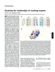
Lemma 2.1 states that there exists a polynomial time transformation that transfers graph G = (V, E) to graph G′ = (V ′ , E ′ ) such that dr(G′ ) ≤ ds(G) + ⌈log2 n⌉ + 3. Proof. Suppose V = {v1 , . . . , vn }, and let d = ⌈log2 n⌉. Construct graph G′ = (V ′ , E ′ ), as Hauptmann et al. [9] do, in the following way (refer to Fig. 2): For every i = 1, . . . , n, V ′ contains a pair of vertices {vi0 , vi1 } and 2(d + 3) vertices uk1 , · · · , ukd+1 , uka , ukb (k = 1, 2). Moreover, V ′ contains an additional vertex c which is connected to all other vertices. The edge set E ′ is defined as follows: vi1 vj1 ∈ E ′ if and only if vi vj ∈ E for i, j = 1, . . . , n; u1k u0k ∈ E ′ for all k = 1, 2, . . . , d + 1, b; vertices u1a and u0a are both adjacent to all 2n vertices vi0 , vi1 , i = 1, . . . , n; vertices vj1 and vj0 are adjacent to u1k and u0k (resp. neither u1k nor u0k ) if the binary representation of j has a 1 (resp. 0) on the k-th position. Suppose without loss 10

of generality that {v1 , . . . , vds(G) } is a minimum dominating set of G. In the following, we show that 1 S := {u11 , · · · , u1d+1 , u1a , u1b } ∪ {v11 , . . . , vds(G) }, the RS given by Hauptmann et al. [9], is actually a DRS of ′ G , which proves the lemma.

Figure 2: The construction of graph G′ Take arbitrary distinct u, v ∈ V ′ . It suffices to show that {u, v} is doubly resolved by S. In view of presence of vertex c, the distance between any pair of vertices in G is at most 2. If at least one of u and v, say u, belongs to S, then {u, v} is doubly resolved by {u, u1b } or {u, u1a } whichever has size 2. Assuming by symmetry |{u, u1b }| = 2, we have dG′ (u, u1b ) − dG′ (u, u) = 2 and dG′ (v, u1b ) − dG′ (v, u) ≤ 1. So we may assume u 6∈ S and v 6∈ S. In case of c ∈ {u, v}, the pair {u, v} is doubly resolved by S as shown by the following: • The pairs {c, vij }, i ∈ {1, . . . , n}, j ∈ {0, 1} are doubly resolved by {u1a , u1b } as dG′ (c, u1b )−dG′ (c, u1a ) = 0 and dG′ (vij , u1b ) − dG′ (vij , u1a ) = 1. • The pairs {c, u0k }, k ∈ {1, . . . , d + 1} are doubly resolved by {u1b , u1k } since dG′ (c, u1b ) − dG′ (c, u1k ) = 0 and dG′ (u0k , u1b ) − dG′ (u0k , u1k ) = 1. • The pair {c, u0b } is doubly resolved by {u1a , u1b } since dG′ (c, u1a ) − dG′ (c, u1b ) = 0 and dG′ (u0b , u1a ) − dG′ (u0b , u1b ) = 1. • The pair {c, u0a } is doubly resolved by {u1b , v11 } since dG′ (c, u1b ) − dG′ (c, v11 ) = 0 and dG′ (u0a , u1b ) − dG′ (u0a , v11 ) = 1. Now we may assume c 6∈ {u, v}. In case of u0k ∈ {u, v} for some k ∈ {1, . . . , d + 1, a, b}, the pair {u, v} is doubly resolved by S as shown by the following: • The pairs {u0k , vij }, i ∈ {1, . . . , n}, j ∈ {0, 1} are doubly resolved by {u1a , u1b } as dG′ (u0k , u1a )−dG′ (u0k , u1b ) = 2 − dG′ (u0k , u1b ) ≥ 0, dG′ (vij , u1a ) − dG′ (vij , u1b ) = −1. • The pair {u0k , u0ℓ } with ℓ ∈ {1, . . . , d+1, a, b}−{k} is doubly resolved by {u1a , u1p }, where p ∈ {k, ℓ}−{a}, since dG′ (u0p , u1p ) − dG′ (u0p , u1a ) = −1 and dG′ (u0q , u1p ) − dG′ (u0q , u1a ) = 2 − dG′ (u0q , u1a ) ≥ 0, where {p, q} = {k, ℓ}. ′

We are left with the case where {u, v} = {vij , vij′ } for some i, i′ ∈ {1, . . . , n} and j, j ′ ∈ {0, 1}. When i 6= i′ , there exists k ∈ {1, 2, . . . , d + 1} such that the binary representations of i and i′ differ at the k-th ′ position (and possibly other positions). The definition of G′ implies {dG′ (vij , u1k ), dG′ (vij′ , u1k )} = {1, 2}. ′ ′ It follows from dG′ (vij , u1a ) = 1 = dG′ (vij′ , u1a ) that {vij , vij′ } is doubly resolved by {u1k , u1a } ⊆ S. When i = i′ , since {v1 , . . . , vds(G) } is a dominating set of G, there exists h ∈ {1, . . . , ds(G)} such that dG (vh , vi ) ≤ 1. Therefore {u, v} = {vi0 , vi1 } is doubly resolved by {vh1 , u1a } because dG′ (vi0 , vh1 ) − dG′ (vi1 , vh1 ) = 1 and dG′ (vi0 , u1a ) − dG′ (vi1 , u1a ) = 0.

C

Approximability

Lemma 3.3 states that IC(T, T0 ) ≥ IC(T, T1 ) for any sets T0 and T1 of super tests with T0 ⊆ T1 .

11

Proof. It has been proved in [1] that IC(T, T0 ) ≥ IC(T, T1 ) if T partitions each equivalence class of ≡T into at most two equivalence classes. Suppose that the equivalence classes of ≡T are E1 , . . . , Em , T partitions each Ei into ki equivalence classes, and k := maxm i=1 ki −1 ≥ 2. We may consider T as k successive tests T1 , . . . , Tk , each of which partitions an equivalence class into at most two equivalence classes. For example, assume that Ei is partitioned into Ei1 , . . . , Eiki by T . We consider Tj (1 ≤ j ≤ ki − 1) partitioning ∪kh=j Eih into Eij i and ∪kh=j+1 Eih , and Tj (ki ≤ j ≤ k − 1) leaving Ei1 , . . . , Eiki unchanged. Using the result in [1] we have IC(T, T0 ) = HT0 −HT0 ∪T = (HT0 −HT0 ∪T1 )+(HT0 ∪T1 −HT0 ∪T1 ∪T2 )+· · ·+(HT0 ∪T1 ∪···∪Tk−1 −HT0 ∪T1 ∪···∪Tk ) ≥ (HT1 − HT1 ∪T1 ) + (HT1 ∪T1 − HT1 ∪T1 ∪T2 ) + · · · + (HT1 ∪T1 ∪···∪Tk−1 − HT1 ∪T1 ∪···∪Tk ) = HT1 − HT1 ∪T1 ∪···∪Tk = HT1 − HT1 ∪T = IC(T, T1 ), as desired. To prove the approximation ratio of Algorithm 1 in Section 3 for finding minimum weighted set of super sets, we need the following lemma from [1]. Lemma C.1 ([1]). If IC(T, T ) > 0 then IC(T, T ) ≥ 1. Theorem 3.4 states that Algorithm 1 is an O(n3 ) time algorithm for the MWSTS problem on (V, Ux ) with approximation ratio Å ã ln max IC(T, ∅) +1 ≤ ln n+ln log2 n+1. T ∈Ux

Proof. Suppose that an optimum solution of the MWSTS problem on (V, Ux ) is T ∗ = {T1∗, . . . , Tk∗ }. The P weight of the solution is ki=1 w(Ti∗ ). During the execution of Algorithm 1, for a current partial P test set ∗ T , let Ti := T + T1 + · · · + Ti∗ (accordingly, T0 = T ) and hi := IC(Ti∗ , Ti−1 ). Notice that ki=1 hi = Pk ∗ i=1 (HTi−1 − HT i−1+Ti∗ ) = HT − HT +T ∗ = HT , since 0 ≤ HT +T ∗ ≤ HT ∗ = 0. Let hi < n log2 n denote the initial value of hi , i.e. the value of hi with T = ∅. During the j-th iteration of the while loop, Algorithm 1 selects a test T (with, say, IC(T, T ) = ∆j ) and P changes T to T +T . As a result, entropy HT drops by ∆j and hi drops by some δi,j such that ki=1 δi,j = ∆j . This iteration adds w(T ) to the solution weight. We distribute w(T ) among the elements of T ∗ by charging each Ti∗ with w(T ) · δi,j /∆j . Recall from Lemma 3.3 that hi = IC(Ti∗ , Ti−1 ) ≤ IC(Ti∗ , T ). By the choice of IC(Ti∗ ,T ) ∆ ) T , we have w(Tj ) = IC(T,T w(T ) ≥ w(Ti∗ ) . Therefore reducing the current hi by δi,j is associated with a charge ∗ that is at most w(Ti ) · δi,j /IC(Ti∗ , T ) ≤ w(Ti∗ ) · δi,j /hi . Let w(h) be the supremum of possible sums of charges that some Ti∗ may receive starting from the time when hi = h > 0. By induction on the number of such positive charges we show w(h) ≤ (1 + ln h) · w(Ti∗ ). If this number is 1, then h > 0 and hence ln h ≥ 0 (by Lemma C.1), while the charge is at most w(Ti∗ ). In the inductive step, we consider the situation, starting with hi = h, where Ti∗ receives a single charge at most w(Ti∗ ) · δ/h, hi is reduced to h − δ > 0 and afterwards. Because of h − δ > 0, Lemma C.1 gives h − δ ≥ 1. By induction assumption, Ti∗ receives at most w(h − δ) charges, and w(h) ≤ w(h − δ) + hδ w(Ti∗ ) ≤ R h−δ dx R h dx (1+ln(h−δ)+ hδ )w(Ti∗ ). Now w(h) ≤ (1+ln h)·w(Ti∗ ) follows from 1+ln(h−δ)+ hδ < (1+ 1 x + h−δ x ) = R h dx 1 + 1 x = 1 + ln h. Recalling h∗i < n log2 n, we have w(h∗i ) < (1 + ln n + ln log2 n) · w(Ti∗ ). This proves our result on the approximation ratio. To implement Algorithm 1, we first compute a table storing the distances between each pair of vertices in G, which takes O(n3 ) time. Having this table, for any given T ∈ Ux − T , it is easy to compute in O(n) time the equivalence classes of ≡T ∪T based the equivalence classes of ≡T . Besides, notice that |Ux | = n − 1 and the while loop is executed at most n times. So the algorithm runs in O(n3 ) time.

D

Cycles

Let G = v1 v2 · · · vn v1 be a cycle, with w(vp ) = minni=1 w(vi ), where p := ⌈n/2⌉. Lemma 4.2 states that Let S be a nonempty subset of V . Then S is a DRS of G if and only if no path in PS has length longer than ⌈n/2⌉ and at least one path in PS has length shorter than n/2. 12

Proof. If there exists one path in PS is longer than ⌈n/2⌉, suppose without loss of generality that this path is v1 v2 · · · v⌈n/2⌉+1 . So from the definition of PS we know, except the two end vertices, there is no other vertex of S on the path. Then we say v1 and v2 can not be doubly resolved by set S, because for any vertex s ∈ S, d(s, v2 ) − d(s, v1 ) = 1. If there is no path in PS has length longer than ⌈n/2⌉ and no path in PS has length shorter than n/2, then it means n is an even number and |S| = 2. Suppose without loss of generality, S = {v1 , v1+n/2 }. Then S can not doubly resolve the pair of vertices {vi , vn−i+2 } for i 6= 1, 1 + n/2. So S is not a DRS. If no path in PS has length longer than ⌈n/2⌉ and at least one path in PS has length shorter than n/2, we show that for any two vertices, they can be doubly resolved by S. For any two vertices u, v ∈ V , if there is no vertex of S on the shortest path from u to v, then it must be the case that u, v are both on one path of PS . Since no path in PS has length longer than ⌈n/2⌉, u, v can be doubly resolved by the two end vertices of that path. If there are two or more vertices of S on the shortest path from u to v, say vi , vj , then (d(u, vi ) − d(u, vj )) · (d(v, vi ) − d(v, vj )) < 0, which implies that u, v are doubly resolved by {vi , vj }. If there is only one vertex vi ∈ S on the shortest path from u to v, then there is another vertex vj ∈ S such that u is on one path of PS , whose two end vertices are vi , vj . If {vi , vj } can doubly resolve u, v, then we are done; Otherwise, d(u, vi ) − d(u, vj ) = d(v, vi ) − d(v, vj ), then it must be the case n = d(u, vi ) + d(u, vj ) + d(v, vi ) + d(v, vj ), so n is an even number and there exists a third vertex vj ′ ∈ S(j 6= j ′ ), s.t. d(u, vi ) − d(v, vi ) 6= d(u, vj ′ ) − d(v, vj ′ ). So S can still doubly resolve {u, v}. Corollary 4.3 states that If some minimum weighted DRS has cardinality 3, then there exists a minimum weighted DRS of G that contains vertex vp . Proof. Suppose without loss of generality {vi , vj , vk } is a minimum weighted DRS, where i < j < p < k. Then from Lemma 4.2, either {vi , vp , vk } or {vi , vj , vp } is a DRS. Since the weight w(vp ) of vp is minimum among all vertices, {vi , vp , vk } or {vi , vj , vp } is also a minimum weighted DRS. Theorem 4.4 states that Algorithm 2 finds in O(n) time a minimum weighted DRS of cycle G. Proof. It suffices to show that at least one of {vi , vi+p−1 }, i = 1, 2, . . . , p, and {vi[j] , vp , uj }, j = 1, 2, . . . , k − 1 is a minimum weighted DRS of G. Notice from Lemma 4.2 that the doubly resolving sets of G that have size two are exactly {vi , vi+p−1 }, i = 1, 2, . . . , p, and all of {vi[j] , vp , uj }, j = 1, 2, . . . , k − 1 are doubly resolving sets of G. It remains to consider the case of three vertices. Suppose that G has no minimum weighted DRS of size two, and by Corollary 4.3 that S = {vℓ , vp , vr } is a minimum weighted DRS. By Lemma 4.2 we may assume 1 ≤ ℓ < p < 1 + p ≤ r ≤ n. If ℓ = i[j] for some 1 ≤ j < k, then Lemma 4.2 implies that r ≥ i[j] + p − 1 and every {vℓ , vp , vh } with vh ∈ Vj is a DRS of G. We may assume that n ≥ r ≥ i[j + 1] + p + 1 as otherwise either {vℓ , vi[j]+p−1 } (when r = i[j] + p − 1) or {vℓ , vp , uj } (when r ∈ Vj ) would be a minimum weighted DRS of G. It follows that {vi[j+1] , vp , vr } is a DRS (by Lemma 4.2), and thus a DRS of weight smaller than w(S) as w(vi[j+1] ) < w(vi[j] ), a contradiction. If i[j] < ℓ < i[j + 1] for some 1 ≤ j ≤ k − 1, then w(vℓ ) ≥ w(vi[j] ) ≥ w(vi[j+1] ). Similar to the above, we have r ≥ ℓ + p. If r ≥ i[j + 1] + p, then {vi[j+1] , vp , vr } is a DRS of G. The minimality of S enforces that w(vi[j+1] ) = w(vℓ ) and {vi[j+1] , vp , vr } is a minimum weighted DRS. As argued in the preceding paragraph, this set must be {vi[j+1] , vp , uj+1 }. Now we are left with the case ℓ + p ≤ r ≤ i[j + 1] + p − 1. Recall that uj is a vertex on the path vi[j]+p vi[j]+p+1 · · · vi[j+1]+p that has minimum weight, saying w(uj ) ≤ w(vr ). It follows that {vi[j] , vp , uj } is a DRS with weight at most that of S. Thus {vi[j] , vp , uj } is also a minimum weighted DRS of G.

E

General k-edge-augmented trees

Observe that G[R ∪ (V \ Vb )] is a forest, where every component is a tree rooted at some unique root in R. Let Tr denote the tree (component) rooted at r ∈ R. In Gb , we change the weights of all roots to zero, while the weights of other vertices remain the same as in G. Next we present the proof of Lemma 4.5.

13

Lemma 4.5 states that Suppose that Sb is a minimum weighted DRS of Gb . Then S = (Sb \ R) ∪ L is a minimum weighted DRS of G. Proof. Using the argument in the proof of Lemma 4.1, we can easily prove L is contained in every DRS of G. Next we prove that S is a DRS of G. Consider any two vertices u, v ∈ R ∪ (V \ Vb ). If |L| ≥ 2, then u, v must be on some shortest path between two leaves of G, which implies that u, v are doubly resolved by these two leaves in L. If |L| = 1, then u, v are on the path from the only leaf, denoted as l, to the only root, denoted as r. Take s ∈ Sb \ {r}. Since d(l, u) − d(l, v) 6= d(r, u) − d(r, v) = d(s, u) − d(s, r) − (d(s, v) − d(s, r)) = d(s, u) − d(s, v), it follows that u, v are doubly resolved by {l, s} (⊆ S = (Sb \ R) ∪ L). Consider any u, v ∈ Vb . Since Sb is a DRS of Gb and dG (u, v) = dGb (u, v), we see that u, v are doubly resolved by Sb in G. If R ∩ Sb = ∅, then u, v are doubly resolved by S. Otherwise, we take r ∈ R ∩ Sb and lr ∈ L ∩ V (Tr ). Since d(lr , u) − d(lr , v) = d(r, u) − d(r, v), it follows that u, v are also doubly resolved by S. Consider any u ∈ Vb \ R and v ∈ V \ Vb . Suppose that v is a vertex of tree Tr , where r ∈ R. There exists a leaf l ∈ L ∩ V (Tr ) such that d(r, l) = d(r, v) + d(v, l). Since r, u ∈ Vb , we have shown in the above that r and u are doubly resolved by S. It follows that there exists s′ ∈ S such that d(u, s′ ) < d(u, r) + d(r, s′ ), as otherwise d(u, s′ ) − d(r, s′ ) = d(u, r) for any s′ ∈ S implies a contraction. From the inequality, we deduce that s′ is not a vertex of tree Tr , saying d(v, s′ ) = d(v, r) + d(r, s′ ). It follows that d(u, s′ ) − d(v, s′ ) < d(u, r) + d(r, s′ ) − (d(v, r) + d(r, s′ )) = d(u, r) − d(v, r). On the other hand, d(u, l) − d(v, l) = =

d(u, r) + d(r, l) − d(v, l) d(u, r) + d(r, v) + d(v, l) − d(v, l) = d(u, r) + d(v, r).

Hence d(u, s′ ) − d(v, s′ ) < d(u, l) − d(v, l), saying that u, v are doubly resolved by {s′ , l} ⊆ S. We have shown that any pair of vertices {u, v} in G can be doubly resolved by S. Thus S is indeed a DRS of G. Now we prove the optimality of S. Suppose on the contrary that S ′ = K ∪ Sb′ is a DRS of G and its weight is smaller than that of S, where K ⊆ V − Vb and Sb′ ⊆ Vb . As mentioned at the beginning of the proof, L ⊆ K, which implies that the weight of Sb′ is smaller than that of Sb . For any w ∈ K and any two vertices u, v ∈ Vb , assume w ∈ Tr for some r ∈ R. We have d(u, w) − d(v, w) = d(u, r) − d(v, r). It follows that R ∪ Sb′ is a DRS of Gb . Note that the weights of vertices in R are 0 in Gb , so the weight of R ∪ Sb′ is smaller than that of Sb . It is a contradiction to the minimality of Sb in Gb . Recall that every vertex of Gb = (Vb , Eb ) has degree at least 2. The following structural property of the base graph has been stated in [7] with a partial proof. We give a full proof for completeness. Lemma E.1. The base graph Gb is decomposed into q ≤ 3k − 3 edge disjoint paths, each of which is a minimal path in Gb with both ends being branching vertices of Gb . P Proof. Observe that Gb is also a k-edge-augmented tree G. Therefore |Eb | = |Vb | − 1 + k, v∈Vb dGb (v) = P P 2|Vb | + 2k − 2 and v∈Vb (dGb (v) − 2) = 2k − 2. It follows that v∈Vb ,dG (v)≥3 dGb (v) ≤ 3(2k − 2). Note that b the degree sum of branching vertices is exactly 2q. Thus 2q ≤ 3(2k − 2) proves the result. In the metric dimension problem, for any minimal RS S ′ , and any path P in the above path decomposition of Gb , it was shown in [7] that the number of vertices in S ′ that are “associated” with P is at most six. Next, we prove an analogue for minimal doubly resolving sets. Lemma E.2. Let S be a minimal DRS of Gb , and let P be a path in the path decomposition of Gb stated in Lemma E.1. Then P contains at most four vertices from S. Proof. Assume on the contrary that there are more than four vertices of S on path P . Note that for any two vertices in Gb , the distance dGb (u, v) between them is d(u, v) the same as that in G. We suppose the two outmost vertices of S on P are s, t and the subpath of P from s to t is v0 v1 · · · vl with v0 = s and vl = t. So dP (vi , vj ) = |j − i| for any i, j ∈ {0.1, . . . , l}. Define 14

i0 := max{i : vi ∈ S and 0 ≤ i ≤ l/2}, j0 := min{i : vi ∈ S and l/2 ≤ i ≤ l}. Obviously, i0 ≤ l/2 ≤ j0 , and by assumption T := (S − V (P )) ∪ {s, vi0 , vj0 , t} is a proper set of S. The minimality of S says that T can not doubly resolve some pair R of vertices of Gb . Write U := {vi : 0 < i < l}. We distinguish among three cases depending on the value of |R ∩ U |, which is 0 or 1 or 2. Case 1. |R ∩ U | = 0. Suppose that R = {u, v}, and {s1 , s2 } doubly resolves R with s1 , s2 ∈ S and s1 6∈ T . If there exists sh ∈ {s1 , s2 }−T such that by switching u and v if necessary we have d(u, sh ) = d(u, s)+dP (s, sh ), d(v, sh ) < d(v, s) + dP (s, sh ) and d(v, sh ) = d(v, t) + dP (t, sh ), d(u, sh ) < d(u, t) + dP (t, sh ), then these four (in)equalities imply d(u, s) − d(v, s) < d(u, sh ) − d(v, sh ) < d(u, t) − d(v, t), saying R is doubly resolved by {s, t}. The contradiction shows that for any sh ∈ {s1 , s2 } − T , there exists rh ∈ {s, t} such that d(u, sh ) = d(u, rh ) + dP (rh , sh ) and d(v, sh ) = d(v, rh ) + dP (rh , sh ), giving d(u, sh ) − d(v, sh ) = d(u, rh ) − d(v, rh ) for every sh ∈ {s1 , s2 } − T. Since R is doubly resolved by {s1 , s2 }, it is easy to see from the above equation that R is doubly resolved by {r1 , r2 } if s2 6∈ T and by {r1 , s2 } otherwise, a contradiction. Case 2. |R ∩ U | = 1. Suppose R = {u, vj } with u ∈ V − U and vj ∈ U . Note that 1 ≤ j ≤ l − 1. In case of j < i0 , note from i ≤ l/2 that dP (vj , vi0 ) = i0 − j < l/2. If d(u, vi0 ) = d(u, s) + dP (s, vi0 ) = d(u, s) + i0 , then R is doubly resolved by {s, vi0 } since d(u, vi0 ) − d(u, s) = i0 > dP (vj , vi0 ) ≥ d(vj , vi0 ) − d(vj , s); otherwise d(u, vi0 ) = d(u, t) + dP (t, vi0 ) = d(u, t) + l − i0 , and R is doubly resolved by {vi0 , t} since d(u, vi0 ) − d(u, t) = l − i0 ≥ l/2 > dP (vj , vi0 ) ≥ d(vj , vi0 ) − d(vj , t). Similarly, in case of j0 < j, we obtain the contradiction that R is doubly resolved by either {t, vj0 } or {vj0 , s}. In case of 0 < i0 ≤ j ≤ j0 < l, let x ∈ {s, t} and y ∈ {vi0 , vj0 } satisfy d(u, x) = min{d(u, s), d(u, t)} and d(vj , y) = min{d(vj , vi0 ), d(vj , vj0 )}. Observe that min{d(u, s), d(u, t)} < min{d(u, vi0 ), d(u, vj0 )} and min{d(vj , vi0 ), d(vj , vj0 )} < min{d(vj , s), d(vj , t)}. It follows that d(u, x) − d(u, y) < 0 < d(vj x) − d(vj , y), contradicting the fact that {x, y} ⊆ {s, t, vi0 , vj0 } ⊆ T does not doubly resolve R. Notice from |S ∩V (P )| > 4 that {i0 , j0 } 6= {0, l}. It remains to consider the case of 0 = i0 < j ≤ j0 < l and that of 0 < i0 ≤ j < j0 = l. By symmetry, it suffices to consider 0 = i0 < j ≤ j0 < l. If d(vj , vj0 ) = d(vj , t)+dP (t, vj0 ), then from the definitions of i0 , j0 it is easy to see that d(vj , v)−d(s, v) = j for every v ∈ S, saying that S does not doubly resolve {vj , s}. The contradiction enforces d(vj , t) + dP (t, vj0 ) > d(vj , vj0 ). If d(u, vj0 ) = d(u, s) + dP (s, vj0 ), then d(u, vj0 ) − d(u, s) = dP (s, vj0 ) > dP (vj , vj0 ) ≥ d(vj , vj0 ) − d(vj , s) shows that R is doubly resolved by {vj0 , s}, a contradiction. Therefore we have d(u, vj0 ) = d(u, t)+dP (t, vj0 ). Since {vj0 , t} does not doubly resolve R = {u, vj }, we have dP (t, vj0 ) = d(vj , vj0 ) − d(vj , t), a contraction to d(vj , t) + dP (t, vj0 ) > d(vj , vj0 ). Case 3. |R ∩ U | = 2. Suppose R = {vi , vj } with 0 < i < j < l. If j ≤ i0 , then R is doubly resolved by {s, vi0 } since i0 ≤ l/2 implies d(s, vi ) − d(s, vj ) = dP (s, vi ) − dP (s, vj ) = i − j and d(vi0 , vi ) − d(vi0 , vj ) = dP (vi0 , vi ) − dP (vi0 , vj ) = j − i. Similarly, if i ≥ j0 , then R would be doubly resolved by {t, vj0 }. Therefore j > i0 and i < j0 . If i < i0 < j ≤ j0 , then the shortest path between vj and s in Gb contains either vi0 or t. In the former case, R is doubly resolved by {s, vi0 } as d(vi , s) − d(vi , vi0 ) = dP (vi , s) − dP (vi , vi0 ) = i − (i0 − i) < i0 and d(vj , s) − d(vj , vi0 ) = dP (vj , s) − dP (vj , vi0 ) = i0 ; in the latter case, R is doubly resolved by {s, t} because d(vi , s) − d(vi , t) < 0 while d(vj , s) − d(vj , t) > 0. Similarly, if i0 ≤ i ≤ j0 < j, then R would be doubly resolved by {t, vj0 } or {t, s}. Hence it must be the case that either i0 ≤ i < j ≤ j0 or i < i0 ≤ j0 < j. If i < i0 ≤ j0 < j, then R is doubly resolved by {s, t} because d(vi , s) = dP (vi , s) ≤ l/2 and d(vj , t) = dP (vj , t) ≤ l/2 imply d(vi , s) − d(vi , t) < 0 < d(vj , s) − d(vj , t). Now we are left with the case of i0 ≤ i < j ≤ j0 . 15

Since {vi0 , vj0 } does not doubly resolve R, there exist x ∈ R = {vi , vj } and y ∈ {vi0 , vj0 } such that some shortest path, denoted as Q, between x and y goes through s and t. If x = vi and y = vi0 , then path Q goes through vi vi+1 · · · vj · · · vj0 vj0 +1 · · · vl−1 vl ; it follows from the definitions of i0 and j0 that all shortest paths between vi and vertices in S go through vj , implying d(vi , v)−d(vj , v) = j −i for every v ∈ S, a contradiction to resolvability of S. Therefore {x, y} 6= {vi , vi0 }, and similarly {x, y} 6= {vj , vj0 }. This particularly says that Gb has only one shortest path between vi and vi0 (resp. vj and vj0 ), which is the one contained in P . Thus d(vi , s) + d(s, vi0 ) > d(vi , vi0 ) and d(vj , t) + d(t, vj0 ) > d(vj , vj0 ). In view that {x, y} is either {vi , vj0 } or {vj , vi0 }, we assume by symmetry that x = vi and y = vj0 . From the shortest path Q = vi vi−1 · · · v0 · · · vl vl−1 . . . vj0 we deduce that d(vi , vj0 ) − d(vi , t) = d(t, vj0 ). Since {vj0 , t} does not doubly resolve R = {vi , vj }, we have d(t, vj0 ) = d(vj , vj0 ) − d(vj , t). However this shows a contradiction to d(vj , t) + d(t, vj0 ) > d(t, vj0 ). The contradictions derived in the above cases prove the lemma. A corollary of Lemmas 4.5, E.1 and Lemma E.2 gives |L| ≤ dr(G) ≤ |L| + 12(k − 1) for k-edge-augmented tree G. On the other hand, it was shown in [7] that md(Gb ) ≤ 18(k − 1). Let graph G′ be obtained from Gb by attaching a pendant edge to each vertex. Then G′ has exactly |Vb | leaves, and dr(G′ ) ≥ |Vb |. Using Lemma 3 of [7], one has md(G′ ) ≤ 18(k − 1), and dr(G′ )/md(G′ ) = Ω(|Vb |) can be arbitrarily large.

F

Wheels

A wheel G = (V, E) on n vertices 1, 2, . . . , n is formed by the hub vertex n and a cycle C = (Vc , Ec ) over the vertices 1, 2, . . . , n − 1, called rim vertices, where the hub is adjacent to some (not necessarily all) rim vertices. The neighbors of hub n are called connectors. The dynamic programming approach has been proved successful in finding minimum weighted resolving sets on wheels [7]. In this section, we show that the approach also works for DRS: a minimum weighted DRS on a wheel can be found in cubic time; the computing time improves to be linear when the wheel is complete. For simplicity, in this section we consider G = (V, E) a (complete or uncomplete) wheel with at least 13 connectors, and design exact algorithms for solving the MWDRS problem on G in cubic time. Observe that wheels with at most 12 connectors are k-edge-augmented trees with k ≤ 12 in which the MWDRS problem is solvable in strongly polynomial time (see Theorem 4.7). The clockwise order of rim vertices along C is 1, 2, . . . , n − 1, 1. Given any rim vertices u and v (possibly u = v), we use C[u, v] to denote the clockwise path of C from u to v. In case of u = v, path C[u, v] consists of a single vertex u. Define C(u, v) := C[u, v] − {u, v}. Let u and v (possibly u = v) be rim vertices. We say that u and v are close to each other if d(u, v) < d(u, n) + d(n, v). We say that rim vertex u is close to vertex subset S if there is s ∈ S such that u is close to s. Suppose that rim vertices u and v are close to each other. We say that u is close to v from the left, equivalently v is close to u from the right, if C[u, v] has length d(u, v). Clearly, a rim vertex is close to itself from both the left and the right. Observe that any two vertices on C[u, v] are closed to each other. This fact and the following observation are frequently used in our discussion implicitly or explicitly. Observation 1. Let s ∈ Vc . The set of vertices which are close to s induces a path Ps of C containing s. Moreover, suppose Ps = C[u, v] is the clockwise path from u to v. Then C[u, s] (resp. C[s, v]) contains at most two connectors. Consider S ⊂ V . If some rim vertex is not close to S, then d(u, s) = d(u, n) + d(n, s) for any s ∈ S, which implies that S can not doubly resolve {u, n}. Consider rim vertices u, v, s. If s is close to neither u nor v, then d(u, s) − d(v, s) = d(u, n) − d(v, n). Apparently we have the following observation. Observation 2. Let S be a DRS of G. The following hold: (i) Every rim vertex is close to S.

16

(ii) For every s ∈ S, if there exist rim vertices u, v close to s such that d(s, u) − d(s, v) = d(n, u) − d(n, v), then there is s′ ∈ S − {s, n} which is close to at least one of u and v such that d(s, u) − d(s, v) 6= d(s′ , u) − d(s′ , v). In our discussion, the additions and subtractions over the vertex indices 1, 2, . . . , n − 1 and ∞ are taken module n − 1. The results of the additions and subtractions are numbers in {1, 2, . . . , n − 1} or ∞ or −∞, where module operation on ∞ (resp. −∞) always produces ∞ (resp. −∞). Lemma F.1. Suppose S ⊆ V is a set to which every rim vertex is close. Then for any rim vertices u, v (possibly u = v) that close to a common vertex s ∈ S, there exists s′ ∈ S − {s} which is close to neither u nor v. Proof. By Observation 1, there are at most 4 connectors contained in C[u, v]. So there are at least 9 connectors on C(v, u), and we can take connector t from C(v, u) such that each of C(v, t] and C[t, u) contains at least 5 connectors. It follows from Observation 1 that Pt = C[x, y] is a proper subpath of D(v, u), each of C(v, x) and C(y, u) contains at least 3 connectors, and Pu ∪ Pv is vertex-disjoint from Pt . Suppose that t is close to s′ ∈ S. Then s′ is contained in Pt , and thus is outside Pu ∪ Pv , saying that s is close to neither u nor v. Lemma F.2. Suppose two rim vertices u, v are both close to rim vertex s and d(u, s) − d(v, s) = d(u, n) − d(v, n). If u is close to rim vertex s′ (6= s), then u, v can be doubly resolved by {s, s′ }. Proof. If v is close to s′ , then Ps and Ps′ both contain u, v, and it is easy to see that u, v are doubly resolved by {s, s′ }. If v is not close to s′ , then d(v, s′ ) = d(v, n) + d(n, s′ ). Using d(u, s′ ) < d(u, n) + d(n, s′ ), we derive d(u, s′ ) − d(v, s′ ) < d(u, n) − d(v, n) = d(u, s) − d(v, s), showing that u, v are doubly resolved by {s, s′ }. Let S (⊆ V ) be a set of observers. Given two distinct rim observers s, s′ ∈ S, we say that s and s′ are consecutive if C(s′ , s) or C(s, s′ ) contains no observer. In the former case, we say that s′ is on the left of s and write s′ = s− ; in the latter case, we say that s′ is on the right of s and write s′ = s+ . Thus the observers contained in C[s− , s+ ] are exactly s− , s and s+ . Given a rim observer s, we call a pair of rim vertices x, y a bad pair of s, if x, y are both close to s, one from the left and one from the right, d(x, s) = d(y, s), and d(x, n) = d(y, n). A bad pair x, y of s is called minimal if d(x, s) = d(y, s) is minimum among all bad pairs of s. We say a minimal bad pair x, y of s is covered by s− from the left if s− is closed to at least one of x and y, and covered by s+ from the right if s+ is closed to at least one of x and y. We say the minimal bad pair of s is covered by S if it is covered by s− or s+ . Let S (⊆ V ) be an observer set and s ∈ S be a rim vertex. We say that S is left-continuous at s if for any rim vertex x ∈ C[s− , s) that is close to s from the left and satisfies 1 = d(x, s) − d(x + 1, s) = d(x, n)−d(x+1, n), we have x close to s− from the right. We say that S is right-continuous at s if for any rim vertex x ∈ C(s, s+ ] that is close to s from the right and satisfies 1 = d(x, s)−d(x−1, s) = d(x, n)−d(x−1, n), we have x close to s+ from the left. Theorem F.3. An observer set S ⊆ V is a DRS of G if and only if the following three conditions are satisfied. (i) Every rim vertex is close to S. (ii) The minimal bad pair of any vertex in S − {n} (if any) is covered by S. (iii) S is left-continuous and right-continuous at every vertex of S − {n}. Proof. To see the “only if” part, suppose that S is a DRS of G. Observations 2(i) gives (i) immediately. If {u, v} is the minimal bad pair of some s ∈ S − {n}, then the condition of Observation 2(ii) is satisfied with d(s, u) − d(s, v) = d(n, u) − d(n, v) = 0, and we have one of u and v close to some s′ ∈ S − {s, n}. Using Observation 1, it is easy to see that one of u and v is close to s− or s+ , establishing (ii). To show the left-continuous of S − {n}, suppose on the contrary that there exists s ∈ S − {n} such that some 17

x ∈ C[s− , s) is close to s from the left, 1 = d(x, s) − d(x + 1, s) = d(x, n) − d(x + 1, n) and x is not close to s− . Then for any s′ ∈ S, either x is not close to s′ or C[x, s′ ] ⊇ C[x, s], giving d(x, s′ ) = d(x, n) + d(n, s′ ) or d(x, s′ ) = d(x, s) + d(s, s′ ). Since d(x, n) = 1 + d(x + 1, n), in either case, some shortest path from x to s′ starts with x(x + 1), giving d(x, s′ ) = 1 + d(x + 1, s′ ), a contradiction to the fact that S doubly resolves {x, x + 1}. Hence S is left-continuous at every s ∈ S − {n}. The right-continuity is proved by a symmetric argument. So (iii) holds. To prove the “if ” part, suppose S ⊆ V satisfies conditions (i) – (iii). Consider an arbitrary pair of vertices {u, v}. We prove that it can be doubly resolved by S. If v = n, then u is a rim vertex, and there must exist s1 , s2 ∈ S such that u is close to s1 (by (i)) but not close to s2 (by Lemma F.1); it is easily checked that u, v are doubly resolved by {s1 , s2 }. If u, v are rim vertices and are not close to any common vertex in S, then by (i) there exist distinct rim vertices s1 , s2 ∈ S such that u is close to s1 but not to s2 and v is close to s2 but not to s1 , which implies d(u, s1 ) − d(v, s1 ) < d(u, n) − d(v, n) < d(u, s2 ) − d(v, s2 ), and thus {u, v} is doubly resolved by s1 , s2 . It remains to consider u, v being both close to some s ∈ S − {n}. Switching u and v if necessary, we may assume C[u, v] ⊆ Ps . If d(u, s) − d(v, s) 6= d(u, n) − d(v, n), then by Lemma F.1, there exists s′ ∈ S − {n} such that neither u nor v is close to s′ , which means d(u, s′ ) − d(v, s′ ) = d(u, n) − d(v, n), and thus {u, v} is doubly resolved by {s, s′ }. So we assume d(u, s) − d(v, s) = d(u, n) − d(v, n),

(F.1)

and distinguish among the following four cases. Case 1. v ∈ C[u, s], i.e., u and v are close to s from the left. Notice from (F.1) that C[u, v − 1] contains no connector. If C(u, s) contains some s′ ∈ S, then u, v are close to s′ , and can be doubly resolved by {s, s′ }. Otherwise, u, v ∈ C(s− , s]. Note that vertex v − 1 on C[u, v) ⊆ Ps is also close to s, and 1 = d(v − 1, s) − d(v, s) = d(v − 1, n) − d(v, n). Since S is left-continuous at s by (iii), vertex v − 1 is close to s− from the right, which implies that u is close to s− . It follows from Lemma F.2 that {u, v} is doubly resolved by {s, s− }. Case 2. u ∈ C[s, v], i.e., u and v are close to s from the left. The proof is similar to that in Case 1, using the right-continuity of S − {n}. Case 3. s ∈ C[u, v] and d(u, s) = d(s, v). Note that u and v form a bad pair of s. From condition (ii), there exists s′ ∈ S − {n} which covers the minimal bad pair of s. It is easy to see that s′ is close to u or v. In turn Lemma F.2 says that {u, v} is doubly resolved by {s, s′ }. Case 4. s ∈ C[u, v] and d(u, s) 6= d(s, v). Suppose without loss of generality that u < s < v and 1 ≤ d(u, s) − d(v, s) = 2s − u − v. It is instant from (F.1) that d(u, n) ≥ 2 and un 6∈ E. Recall that every vertex in C[u, s] is close to u and every vertex in C[s, v] is close to v. In view of (F.1) and Lemma F.2, we only need to consider the case of C[u, v] ∩ S = {s}, i.e., s− , s+ ∈ C(v, u). If there exists a vertex x on C[u, s) ⊆ Ps such that d(x, n) − d(x + 1, n) = 1, then x is closed to s from the left, and 1 = d(x, s) − d(x + 1, s) = d(x, n) − d(x + 1, n). Since S is left-continuous at s, vertex x is close to s− from the right. It follows that u is close to s− . Thus lemma F.2 says that {u, v} is doubly resolved by {s, s− }. In the remaining proof, we assume that there does not exist such an x on C[u, s), implying d(x, n) ≤ d(x + 1, n) for every x ∈ C[u, s). Particularly, d(s − 1, n) ≤ d(s, n). Then either all vertices on C[u, v) are connectors or none of them is a connector. Since un 6∈ E, we see that C[u, s) contains no connector, and d(s − 1, n) = d(s − 2, n) + 1 = · · · = d(u, n) + s − 1 − u. So d(u, n) + s − 1 − u ≤ d(s, n) ≤ d(s, v) + d(v, n) = v − s+ d(v, n), yielding d(u, n)− d(v, n)+ 2s− u − v ≤ 1. It follows from (F.1) and d(u, s)− d(v, s) = 2s− u − v that 2(d(u, s) − d(v, s)) ≤ 1, a contradiction to d(u, s) − d(v, s) ≥ 1. From Theorem F.3, we have the following corollary.

18

Corollary F.4. If S ⊆ V is a minimal DRS, then n 6∈ S. There are two major different features between the characterizations of minimal doubly resolving sets and minimal resolving sets on wheels. First, some consecutive rim vertices are allowed to be not close to the RS. So when designing the dynamic programming algorithm for finding minimum weighted RS, Epstein et al. [7] could choose a feasible pair of start and end vertices, without considering the stop condition. Second, to find a feasible RS, it suffices to consider the bad pair case of an observer vertex, while to find a feasible DRS, we additionally need to make sure that the set under consideration is left-continuous and right-continuous at every observer vertex. Both differences make the algorithm design for the MWDRS problem more complex and difficult. Next we design a strongly polynomial time dynamic programming algorithm to find a minimum weighted DRS of G. Let a be a rim vertex such that Pa is shortest among all rim vertices. Note that every minimum weighted DRS must contain some vertex from Pa . By examining all vertices in Pa , without loss of generality we assume that vertex 1 ∈ V (Pa ) is an observer in a minimum weighted DRS. Our aim is to construct an observer set S of minimum weight on the condition that 1 ∈ S and S satisfies conditions (i)–(iv) in Theorem F.3. Such an S must be a minimum weighted DRS of G as guaranteed by Theorem F.3. Henceforth we assume 1 ∈ S. Before describing our algorithm, we introduce some notations. Let l1 and r1 to be the rim vertices such that C[l1 , r1 ] = P1 is the path induced by all vertices close to vertex 1. For any rim vertex u with 1 < u ≤ n − 1, suppose we put u into S. To assure validity of conditions (ii)-(iv) of Theorem F.3, basically we need check every vertex in Pu . But by virtue of 1 ∈ S, we can narrow the range Pu by cutting off its intersection with P1 . Let lu ≥ 1 be the minimum index and ru ≤ n − 1 be the maximum index such that C[lu , ru ] is a subpath of Pu (so all vertices on C[lu , ru ] are close to u). Let 1 ≤ v ≤ n − 1. • If there exists 1 ≤ j < n − 2 such that v − j ∈ C[lv , v) (so v − j is close to v from the left) and d(v − j, v) − d(v − j + 1, v) = 1 = d(v − j, n) − d(v − j + 1, n), then let ∆l (v) denote such a minimum j; otherwise, set ∆l (v) := ∞. • If there exists 1 ≤ j < n − 2 such that vertex v + j ∈ C(v, rv ] (so v + j is close to v from the right) and d(v + j, v) − d(v + j − 1, v) = 1 = d(v + j, n) − d(v + j − 1, n), then let ∆r (v) denote such a minimum j; otherwise, set ∆r (v) := ∞. • If there exists 1 ≤ j < n − 2 such that v − j, v + j form a bad pair contained in C[lv , rv ], then let ∆(v) denote such a minimum j; otherwise, set ∆(v) := ∞. Observation 3. Let S (⊆ V − {n}) be a set of rim observers, and let s ∈ S. (i) If rs− ≥ ls − 1, then every vertex of C[s− , s] is close to {s− , s}. (ii) If rs− ≥ s − ∆l (s), then S is left-continuous at s. (iii) If ls+ ≤ s + ∆r (s), then S is right-continuous at s. (iv) If rs− ≥ s − ∆(s), then s− covers the minimal bad pair of s (if any) from the left. (v) If ls+ ≤ s + ∆(s), then s+ covers the minimal bad pair of s (if any) from the right. We define two functions F and F ′ from {1, 2, . . . , n − 1} × {left, right} to R+ as follows: The functions map (s, ·) to the minimum weight of a vertex set S ⊆ {1, . . . , s} satisfying (a) 1, s ∈ S; (b) every vertex i with 1 ≤ v ≤ s is close to S; (c) S is left-continuous at every vertex of S − {1}, and right-continuous at every vertex of S − {s}. (d) for F (s, left) (resp. F ′ (s, left)), the minimal bad pair of any vertex in S (resp. S − {1}) is covered by S, and the minimal bad pair of s (if any) is covered by s− from the left, (e) for F (s, right) (resp. F ′ (s, right)), the minimal bad pair of any vertex in S − {s} (resp. S − {1, s}) is covered by S, and the minimal bad pair of s (if any) will be covered from the right later. 19

Correspondingly, for F (s, ·) (resp. F ′ (s, ·)), let S(s, ·) (resp. S ′ (s, ·)) denote the minimum weighted S described above. Algorithm 3. Finding minimum weighted DRS of general wheels Using dynamic program, we compute the values of F (s, ·) and F ′ (s, ·) recursively for s = 1, 2, . . . , n − 1. The initial settings are 1. Initial Step: F (1, left) := ∞ and F (1, right) = F ′ (1, left) = F ′ (1, right) := c(1). For s > 1, we need select s′ from {1, 2, . . . , s − 1} and S ′ ∈ {S(s′ , left), S ′ (s′ , left), S(s′ , right), S ′ (s′ , right)} such that S = S ′ ∪ {s} is the minimum weighted set satisfying (a) – (d). In view of Observation 3, we define α(s) := {s′ ∈ {1, 2, . . . , s − 1} : rs′ ≥ ls − 1, rs′ ≥ s − ∆l (s), s′ + ∆r (s′ ) ≥ ls }, β(s) := {s′ ∈ α(s) : rs′ ≥ s − ∆(s)} ⊆ α(s), γ(s) := {s′ ∈ α(s) : ls ≤ s′ + ∆(s′ )} ⊆ α(s). From Observation 3(i)-(iii), it is easy to see that (a), (b) and (c) are satisfied as long as we take s′ from α(s). Note that S(s, left) − {s} is either S(s′ , left) or S(s′ , right) for some s′ ≤ s − 1, In the former case, we only need to guarantee that the minimal bad pair of s (if any) is covered by s′ . Observation 3(iv) says that s′ ∈ β(s) suffices. In the latter case, we are done if we additionally make sure that the minimal bad pair of s′ (if any) is covered by s. This, by Observation 3(v), is equivalent to requiring s′ ∈ γ(s). Hence we obtain 2. Recursive Step:  F (s, left) = min mins′ ∈β(s) F (s′ , left), mins′ ∈β(s)∩γ(s) F (s′ , right) + c(s)

Similarly, we have other recursive formulas for computing F and F ′ as follows 3. Recursive Step: F (s, right) = min

ß

™ ′ ′ min F (s , left), min F (s , right) + c(s) ′ ′

s ∈α(s)

4. Recursive Step: ß F ′ (s, left) = min ′min F ′ (s′ , left), s ∈β(s)

s ∈γ(s)

min

s′ ∈β(s)∩γ(s)

™ F ′ (s′ , right) + c(s)

5. Recursive Step: + c(s),  c(1) ß ™ F ′ (s, right) = ′ ′ ′ ′ min min F (s , left), min F (s , right) + c(s),  ′ ′ s ∈α(s)

s ∈γ(s)

1 ∈ α(s) 1 6∈ α(s)

When the recursive formulas stop at s = n − 1, we are ready to give the weight of minimum weighted DRS assuming vertex 1 is an observer. For vertex 1, note that 1 − ∆l (1) ≡ n − ∆l (1) (mod n − 1) and 1 − ∆(1) ≡ n − ∆(1) (mod n − 1). We define the sets of possible consecutive observers on the left of vertex 1 as α(1) = {s ∈ {2, 3, . . . , n − 1} : rs ≥ l1 − 1, rs ≥ n − ∆l (1), s + ∆r (s) ≥ l1 }, β(1) = {s ∈ α(1) : rs ≥ n − ∆(1)}, γ(1) = {s ∈ α(1) : l1 ≤ s + ∆(s)}. In particular, picking s = 1− from α(1) guarantees that S is left-continuous at 1. Furthermore, combining (a)–(e) and Observation 3, we deduce from Theorem F.3 that the minimum weighted DRS of G must be one of S(s, left) with s ∈ α(1), S ′ (s, left) with s ∈ β(1), S(s, right) with s ∈ γ(1), and S ′ (s, right) with s ∈ β(1) ∩ γ(1). These sets satisfy all the conditions in Theorem F.3. Hence the weight of the optimal DRS is given by 20

6. Finalß Step: min min F (s, left), min F ′ (s, left), min F (s, right), s∈α(1)

s∈β(1)

s∈γ(1)

min

™ F ′ (s, right) .

s∈β(1)∩γ(1)

By backtracking we can get the optimal set. To summarize, Steps 1-6 present our dynamic programming algorithm for finding minimum weighted DRS in wheels. Its correctness follows from the description and corresponding analysis. Theorem F.5. The MWDRS problem on general wheels can be solved in O(n3 ) time.

21