Approximate operations in Convolutional Neural Networks with RNS

ESANN 2017 proceedings, European Symposium on Artificial Neural Networks, Computational Intelligence and Machine Learning. Bruges (Belgium), 26-28 April 2017, i6doc.com publ., ISBN 978-287587039-1. Available from http://www.i6doc.com/en/.

Approximate operations in Convolutional Neural Networks with RNS data representation Valentina Arrigoni1 , Beatrice Rossi2 , Pasqualina Fragneto2 Giuseppe Desoli2 1- Universit` a degli Studi di Milano - Dipartimento di Matematica via Saldini 50, Milan - Italy 2- STMicroelectronics - AST via Olivetti 2, Agrate Brianza - Italy Abstract. In this work we modify the inference stage of a generic CNN by approximating computations using a data representation based on a Residue Number System at low-precision and introducing rescaling stages for weights and activations. In particular, we exploit an innovative procedure to tune up the system parameters that handles the reduced resolution while minimizing rounding and overflow errors. Our method decreases the hardware complexity of dot product operators and enables a parallelized implementation operating on values represented with few bits, with minimal loss in the overall accuracy of the network.

1

Introduction

Convolutional Neural Networks (CNNs) are neural networks that combine a deep multi-layer neuron model with convolutional layers. Nowadays CNNs are widely exploited in mobile and embedded systems (e.g. low-power wearable or IoT devices), for a number of applications that require real-time processing. In these systems, the learning stage is performed offline and pre-trained CNNs are exploited when executing the runtime mode. The inference stage of CNNs is dominated in complexity by convolutions (convolutional layers contain more than 90% of the total required computations). In convolutional layers, and also in fully connected ones, the key arithmetic operation is the dot product followed by the addition of the bias z = wT a+b, where a ∈ Rn are the input activations, w ∈ Rn the corresponding weights and b is the bias. Dot products can be computed through n multiply-accumulate operations, each of which computes the product of two operands and adds the result to an accumulator at a specific resolution (e.g. 32 bits for 16 bits operands). The hardware (HW) unit that performs this operation is known as a multiplier-accumulator (MAC or MAC unit). In CNNs the number of total dot products is relatively high, for example, for a 224x224 image, a single category labeling classification with 1000 classes requires close to 1 Giga operations using AlexNet [1]. Due to computational complexity and speed requirements, many proposals for HW acceleration of CNNs are surfacing. In particular, in order for large CNNs to run in real-time on resource-constrained systems, it is of crucial importance to simplify/approximate MAC units since they are usually responsible for significant area, power and latency costs. This work is grounded on the well-established principle that algorithmic-level noise resiliency of CNNs can promote low-precision arithmetic and simplifica-

583

ESANN 2017 proceedings, European Symposium on Artificial Neural Networks, Computational Intelligence and Machine Learning. Bruges (Belgium), 26-28 April 2017, i6doc.com publ., ISBN 978-287587039-1. Available from http://www.i6doc.com/en/.

tions in HW complexity [2, 3, 4]. In particular, we propose to modify the inference stage of a generic CNN by approximating computations using a nonconventional data representation based on a Residue Number System (RNS) [5] at low-precision and introducing stages for rescaling weights and activations. We present a novel procedure for tuning the RNS parameters that copes with the reduced resolution of data and accumulators and minimizes rounding and overflow errors. Our approach decreases dot product HW implementation costs enabling a parallelized design operating on narrowly defined values represented with few bits, without a significant decrease of the overall accuracy of the network. 1.1

Related Works

In the last years, several approaches have been proposed to accelerate the inference stage of CNNs. A first class of methods makes use of low-precision arithmetic and quantization techniques [2, 6, 3, 4]. Another strategy is to exploit the redundancy within the convolutional filters to derive compressed models that speed up computations [7, 8]. A third class of techniques proposes HW-specific optimizations [9, 2, 10, 11]. The works [4] and [11] are the more closely related to our solution. In [4] a non-conventional data representation based on a base2 logarithmic system is proposed. Weights and activations are represented at low precision in the log-domain obviating the need for digital multipliers (multiplications become additions in the log-domain) and obtaining higher accuracy than fixed-point at the same resolution. However, this solution merely takes advantage of recasting dot products in the log-domain, while it still requires accumulators at full precision (e.g. 32 bits). As for the log-domain representation, albeit showing a good complexity reduction potential, a fully documented analisys in terms of the costs associated to the HW implementation of a complete chain of processing in a convolutional stage is not available. In [11] a non-conventional data representation based on a Nested Residue Number System (NRNS) (a variant of RNS) is proposed. A 48-bit fixed-point representation is used for weights and activations, and dot products of convolutional layers are computed in parallel using an NRNS at high precision in order to cover a maximum dynamic range of 2103 . By applying NRNS, standard MAC units are decomposed into parallel 4-bit MACs. Our RNS representation approach differs in exploiting the CNN error propagation resiliency by setting an RNS at lowprecision and properly tuning rescaling stages in order to handle the reduced resolution of data and accumulators and to maximize accuracy.

2 2.1

Proposed Solution Mathematical Background

A Residue Number System is defined by a set of integers (mN , . . . , m1 ) called base, where every integer mi is called modulus. It is an integer system in which the size of the dynamic range is given by the least common multiple of the moduli, and it is denoted by M . A number x ∈ Z is represented in the RNS by

584

ESANN 2017 proceedings, European Symposium on Artificial Neural Networks, Computational Intelligence and Machine Learning. Bruges (Belgium), 26-28 April 2017, i6doc.com publ., ISBN 978-287587039-1. Available from http://www.i6doc.com/en/.

the set of residues (xN , . . . , x1 ) where xi := |x|mi = x mod mi ∈ {0, 1, . . . , mi − 1}. In order to have a unique corresponding value for each RNS number, a RNS can be accompanied with a range denoted by IRN S = [r, r + M − 1] ⊆ Z. In this way, a given RNS number (xN , . . . , x1 ) is converted to x = v if v ∈ IRN S , or x = v − M otherwise, where v is obtained by applying the Chinese Remainder Theorem [5], under the assumption that moduli are pairwise coprime. Some arithmetic operations in the RNS are simplified, in particular additions, subtractions and multiplications. Indeed, these operations can be computed digit-wise, i.e. by considering the residues of the operands separately for each modulus. In our proposal, the operation performed in residual domain is the dot product followed by the addition of the bias. Let w = [w1 , . . . , wn ]T and a = [a1 , . . . , an ]T be two vectors with integral components, and let b an integer. The components of the RNS representation of z = wT a + b can be computed as     i = 1, . . . , N. (1) zi =  N j=1 |wj |mi · |aj |mi + |b|mi  mi

Note that, according to Eq. (1), the operation z = wT a + b can be decomposed into N operations of small sizes, one for each modulus, enabling a parallelized implementation. As for the choice of the moduli, a set of comprime moduli of the form {21 , 22 − 1, . . . , 2N − 1} allows for an efficient storage and further simplifies arithmetic operations. For more details on RNS see [5]. 2.2

Outline of the Method

In our proposal, we start from a CNN with pre-trained weights and we properly select some operations of the forward propagation to be computed in residual domain, meaning that only numbers in RNS representations are involved. The parts in which we perform computations in RNS are called residual blocks, and consist of convolutions or matrix products followed by the addition of the bias. As a consequence, operations in residual blocks are all of the form z = wT a + b. In the other parts computations are performed as usual, in standard domain. We set a fixed low-precision resolution for data and accumulators (e.g. 16 bits), and for each residual block we select the same RNS base with coprime N moduli of the form {21 , 22 − 1, . . . , 2N − 1} such that i=1 i equals the resolution. Observe that, within each residual block, the possible errors derive from the rounding of weights and activations (necessary in order to convert them in RNS) and from overflows. The k-th residual block is associated to a couple of pa(k) (k) rameters, (λw , λa ), defined as expansion factors for which we multiply weights, activations and biases before rounding and converting them in RNS. The k-th   (k) residual block is also associated to a specific range, IRN S = r(k) , r(k) + M − 1 parametrized by r(k) . All these parameters need to be properly tuned in order to contain both overflow and rounding errors, aiming at maximizing the accuracy. The scheme of the k-th residual block can be summarized as follows. Acti(k) vations from the previous layer are multiplied by λa , rounded and converted (k) (k) (k) in RNS. Conversely, weights and biases are multiplied by λw and λw λa re-

585

ESANN 2017 proceedings, European Symposium on Artificial Neural Networks, Computational Intelligence and Machine Learning. Bruges (Belgium), 26-28 April 2017, i6doc.com publ., ISBN 978-287587039-1. Available from http://www.i6doc.com/en/.

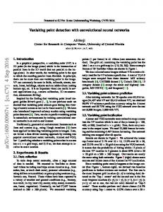
(k)

Fig. 1: On the left, selection of λ0.8 : the histogram of v (k) is expanded by the (k) factor λ0.8 = 4 in order to have |I˜(k) |  0.8M , where M = 400. On the right, (k) (k) selection of the RNS range IRN S corresponding to λ0.8 = 4: the range I˜(k) of v˜(k) is [−36, 280] and the mean is 48.2155, thus the value r(k) = −97 is computed. spectively, rounded, converted in RNS offline and then stored. The results are (k) (k) computed in RNS, converted in standard domain and then divided by λw λa . 2.3

Parameter Tuning

Considering the layer k, the basic idea behind the tuning of the parameters (k) (k) (λw , λa ) and r(k) consists in containing rounding errors and at the same time (k) reducing overflow occurrences. We first compute the minimum values λwmin (k) and λamin for which the rounding errors do not impact significantly on the CNN (k) (k) accuracy. This is done by testing sample values for λw and λa separately (setting to a large value the other factor) and evaluating the performance of an auxiliary CNN in which only the k-th block performs the product by the expansion factors and the rounding, and all operations are at high precision. Then we select a random subset of the validation set and we perform the inference on the standard CNN in order to estimate the distribution of values corresponding to the output of the k-th residual block. The partial values are (k) stored in a vector v (k) . We compute the value λ0.8 for which |I˜(k) | = 0.8M , (k) (k) where I˜(k) = [min(v (k) )λ0.8 , max(v (k) )λ0.8 ] is the estimated output range of (k) (k) (k) (k) (k) the block. If M is large enough to have λ0.8 ≥ λwmin λamin , we set (λw , λa ) (k) (k) (k) (k) (k) (k) (k) such that they satisfy equations λw λa = λ0.8 and λw λamin = λa λwmin . Oth(k) (k) (k) (k) (k) erwise, if λ0.8 < λwmin λamin , we test increasing sample values for λw and λa starting from the minima and we chose those that maximize the accuracy. We tune the parameter r(k) in the following way. If |I˜(k) | < M , we force (k) (k) IRN S to contain I˜(k) and we distribute the |IRN S \ I˜(k) | remaining values to the left or the right of I˜(k) so to minimize the probability of overflows. In particular, (k) (k) we first compute v˜(k) = v k · (λw λa ), the estimated output distribution of the k-th residual block or equivalently the distribution of values computed by the

586

ESANN 2017 proceedings, European Symposium on Artificial Neural Networks, Computational Intelligence and Machine Learning. Bruges (Belgium), 26-28 April 2017, i6doc.com publ., ISBN 978-287587039-1. Available from http://www.i6doc.com/en/.

accumulators. Then we set r(k) = m(k) − (1 − d(k) /|I˜(k) |) · (M − |I˜(k) |) − 1, v (k) )|. If |I˜(k) | > M , we set where m(k) = min(I˜(k) ) and d(k) = |m(k) − mean(˜ (k) (k) r in order to maximize the percentage of values of v˜(k) included in IRN S . An (k) example of parameter tuning for the case |I˜ | < M is in Fig. 1.

3 3.1

Results Hardware Implementation

We have made a preliminary implementation of the multiply-accumulate operators (RNS MAC units) in residual domain. Our operators have three 16 bits inputs for weights, activations and accumulator input and one accumulator output. The RNS MAC unit is composed by separated data-paths, one for each modulus bit range representation out of a 16 bits vector. The dot product associated to the modulus 2i is implemented with a standard MAC while the other moduli need a special treatment to accommodate the modular arithmetic involving end-around-carry handling (our approach is relatively conventional with respect to the state of the art modulo 2i − 1 fused multiply add units such as in [12]). While not yet taking full advantage of the benefit of delayed carry representation followed by an end-around-carry CSA tree and modulo adder, the scaling advantages of such an approach would be limited for narrow units such as the one proposed. Comparison were made against an optimized MAC unit with 16 bits operands and 32 bits accumulator input/output in a 28nm technology library setting design constraints for timing at 500 MHz for purely combinatorial units and at 2 GHz for pipelined version. Results show for RNS MAC units benefits in terms of area reduction from 2-4x (2.53 for the base (23 , 26 − 1, 27 − 1)) for both combinatorial and pipelined. Timing for RNS MAC units is 1.5-2.4x faster while total estimated power consumption savings range from 3x to 9x. 3.2

Accuracy Evaluation

As for accuracy, we evaluated our method on the CNN AlexNet, proposed in [1] for classifying images from the ImageNet LSVRC-2010 contest into 1000 classes. In particular, we replicated in MATLAB the inference stage of AlexNet, using the version provided by the Caffe Model Zoo [13], for which trained weights are available. We set the resolution to 16 bits, and the RNS base to (23 , 26 − 1, 27 − 1), (k) which provides M = 64008. Moreover, we also verified that setting λa = 1 for k = 1, . . . , 8 does not affect significantly the network accuracy. We then implemented the procedure for tuning of the remaining parameters, starting from (k) λw for k = 1, . . . , 8, for which the network is particularly sensitive, and then selecting the RNS range for each residual block accordingly. We also replicated the above procedure considering the expansion factors as powers of two. This choice allows to further simplify the division by the product of the factors at the end of the residual block in view of an optimized hardware implementation. The performances of AlexNet on the validation set, following our proposed method and this last variation, are reported in Table 1.

587

ESANN 2017 proceedings, European Symposium on Artificial Neural Networks, Computational Intelligence and Machine Learning. Bruges (Belgium), 26-28 April 2017, i6doc.com publ., ISBN 978-287587039-1. Available from http://www.i6doc.com/en/.

top5(%) top1(%)

RNS AlexNet 75.09 51.33

RNS AlexNet (variation) 76.24 52.60

original AlexNet 79.12 55.78

Table 1: Accuracy of AlexNet. In the third column, the variation refers to the case where expansion factors are powers of two.

4

Conclusions

In this paper we described an RNS based representation for weights and activations in CNNs, along with a modified inference stage associated with an algorithmic procedure to tune up RNS parameters for best accuracy. Synthesis results, for area, power and timing, from a preliminary HW implementation of the resulting MAC units in the residual domain are encouraging, as well as the ensuing overall accuracy of the network (we obtained a drop of at worst 4% in top5 and top1 accuracy).

References [1] Alex Krizhevsky, Ilya Sutskever, and Geoffrey E Hinton. Imagenet classification with deep convolutional neural networks. In Adv Neural Inform Process Syst, 2012. [2] Vincent Vanhoucke, Andrew Senior, and Mark Z Mao. Improving the speed of neural networks on cpus. In Proc. of Deep Learning and Unsupervised Feature Learning Workshop, NIPS, 2011. [3] Martın Abadi et al. Tensorflow: Large-scale machine learning on heterogeneous distributed systems. arXiv preprint arXiv:1603.04467, 2016. [4] Daisuke Miyashita, Edward H Lee, and Boris Murmann. Convolutional neural networks using logarithmic data representation. arXiv preprint arXiv:1603.01025, 2016. [5] Nicholas S Szabo and Richard I Tanaka. Residue arithmetic and its applications to computer technology. McGraw-Hill, 1967. [6] Song Han, Jeff Pool, John Tran, and William Dally. Learning both weights and connections for efficient neural network. In Adv Neural Inform Process Syst, 2015. [7] Emily L Denton, Wojciech Zaremba, Joan Bruna, Yann LeCun, and Rob Fergus. Exploiting linear structure within convolutional networks for efficient evaluation. In Adv Neural Inform Process Syst, 2014. [8] Max Jaderberg, Andrea Vedaldi, and Andrew Zisserman. Speeding up convolutional neural networks with low rank expansions. arXiv preprint arXiv:1405.3866, 2014. [9] Cl´ ement Farabet, Berin Martini, Polina Akselrod, Sel¸cuk Talay, Yann LeCun, and Eugenio Culurciello. Hardware accelerated convolutional neural networks for synthetic vision systems. In Proc. of 2010 IEEE International Symposium on Circuits and Systems, 2010. [10] Michael Mathieu, Mikael Henaff, and Yann LeCun. Fast training of convolutional networks through ffts. arXiv preprint arXiv:1312.5851, 2013. [11] Hiroki Nakahara and Tsutomu Sasao. A deep convolutional neural network based on nested residue number system. In International Conference on Field Programmable Logic and Applications, 2015. [12] Constantinos Efstathiou, Kostas Tsoumanis, Kiamal Pekmestzi, and Ioannis Voyiatzis. Modulo 2n±1 fused add-multiply units. In 2015 IEEE Computer Society Annual Symposium on VLSI, pages 91–96. IEEE, 2015. [13] http://caffe.berkeleyvision.org/model_zoo.html.

588