Payame Noor University
Journal of Control and Optimization in Applied Mathematics (JCOAM) Vol. 1, No. 1, Spring-Summer 2015(1-19), ©2015 Payame Noor University, Iran
Approximate Pareto Optimal Solutions of Multi-objective Optimal Control Problems by Evolutionary Algorithms A. H. Borzabadi1∗ , M. Hasanabadi2 and N. Sadjadi3 1,2 School
of Mathematics and Computer Science, Damghan University, Damghan, Iran 3 C Real de Burgos, University of Valladolid, Valladolid, Spain Received: March 3, 2014; Accepted: July 15, 2014.
Abstract. In this paper an approach based on evolutionary algorithms to find Pareto optimal pair of state and control for multiobjective optimal control problems (MOOCP)’s is introduced. In this approach, first a discretized form of the time-control space is considered and then, a piecewise linear control and a piecewise linear trajectory are obtained from the discretized time-control space using a numerical method. To do that, a modified version of two famous evolutionary genetic algorithm (GA) and particle swarm optimization (PSO) to obtain Pareto optimal solutions of the problem is employed. Numerical examples are presented to show the efficiency of the given approach.
Keywords. Multi-objective optimal control problem, Pareto solution, Evolutionary algorithm, Discretization, Approximation. MSC. 49M30; 92-08.
∗ Corresponding author
[email protected],
[email protected],
[email protected] http://mathco.journals.pnu.ac.ir
2
Approximate Pareto Optimal Solutions .../ JCOAM, 1(1), Spring-Summer 2015
1 Introduction
In many practical or real life problems, we normally need to optimize several objectives simultaneously, which can even be in conflict to each other. In engineering and economics, we encounter the same situation that many optimization problems involve Multi-objectives cost functions. For example, one might want to adjust a rocket’s fuel usage and orientation so that it arrives at a specified place and at a specified time; or one might want to conduct open market operations so that both the inflation rate and the unemployment rate are as close as possible to their desired values ( see for various applications [3, 13, 23, 27]). In these problems, however, instead of a single optimum there are rather a set of alternative trade-offs, generally known as Pareto optimal solutions, which are considered to be equally important, since all of them constitute global optimum solutions and hence a variety of methods have been developed for the solution of multi-objective optimization problems. In the area of control engineering, multi-objective optimization discussion has been used by the control engineers (see e.g. [6, 10, 20]). Targeted to manage many objectives, which often involves conflict situations of many criteria, such as control energy, tracking performance, robustness, etc. A suitable introduction on the concepts of MOOCP may be found in ([11]). Also, one may find an overview on multi-objective optimization applications in control engineering in ([20]). Over the years, some indirect and direct approaches with different views including Q-parametrization ([14]), Chebyshev spectral procedure ([9]), nonessential functional ([1]), extending the state space ([18]) and scalarizing objectives ([4]) have been presented to extract analytical and approximate Pareto solutions of MOOCP’s. But, these approaches are facing some difficulties the same of the methods which have been proposed for single-objective optimal control problems. For instance, in algorithm based on parameterization and scalarization, the region of Pareto solutions can be surrounded related to the scheme of scalarizing or another instance of difficulty is that in some of these methods, convexity of the objectives is a basic requirement which limits the scope of applications of such methods. There from that the study of multi-objective optimization has flourished to a level where uncertainty is considered when comparing and evaluating solutions for any given problem, this development has been generalized to the area of MOOCP’s (see e.g., [22, 29]).
A. H. Borzabadi, M. Hasanabadi, N. Sadjadi/ JCOAM, 1(1), Spring-Summer 2015
3
Although the above mentioned methods suffer from some difficulties, recently several evolutionary methodologies could show good performance detect approximate solutions of multi-objective problems, such as Non-dominated Sorting Genetic Algorithm NSGA ([26]), NSGA-II ( [7]), Strength Pareto Evolutionary Algorithm SPEA ([32]), SPEA2 ( [31]), Pareto Archive Evolution Strategy PAES ([17]), Multi-Objective Particle Swarm Optimization (MOPSO) ([5]) and MultiObjective Invasive Weed Optimization (MOIWO) ([19]). Analytical discussion on a class of these problems can be found in ([2]). Also there are some approaches based on bacterial chemotaxis ([12]), networks theory ([16]), weighted optimization ([24]) and scalarization ([28]) which are presented to extract approximate solution of these problems based on different concepts. Due to outstanding abilities of evolutionary algorithms in finding Pareto solutions of multi-objective optimization problems, in this paper we propose an approach based on evolutionary algorithms to find a Pareto optimal pair of state and control for multi-objective optimal control problems. The considered multi-objective optimal control problem formulation requires the simultaneous minimization of m objective in contrast to the general optimal control problem formulation, in which only one objective has to be minimized. In mathematics, it is
min x(·),u(·),T
s.t :
{φ1 (x(.), u(.), T ), . . . , φj (x(·), u(·), T ), . . . , φm (x(·), u(·), T )}
(1)
F (t, x(t), x(t), ˙ u(t)) = 0,
(2)
h(t, x(t), u(t)) ≥ 0,
(3)
r(x(0), x(T )) = 0.
(4)
Here, function F represents the model equation with x as model states, u as control inputs, and T as the final time. Also, φj denotes the j-th individual objective functional as ∫ φj (x(.), u(.), T ) =
T
fj (t, x(t), u(t))dt, 0
with continuous function fj , while h and r are the path constraints and boundary constraints of the optimal control problem.
4
Approximate Pareto Optimal Solutions .../ JCOAM, 1(1), Spring-Summer 2015
2 Discretization of the Control Space To determine the optimal solution we must examine the performance index in the set of all possibilities of control-state pairs. The set of admissible pairs consisting of pairs like (x, u) satisfying (1)-(4) is denoted by P . In this section we present a control discretization method based on an equidistant partition of [0, T ] as t −t ∆t = {0 = t0 , t1 , . . . , tn−1 , tn = T } with discretization parameter h = n n 0 . The time interval is divided into n subinterval [t0 = 0, t1 ], [t1 , t2 ], . . . , [tn−1 , tn = T ]. On the other hand, corresponding to i-th component of control vector function the set of control values is divided into constants ui0 , ui1 , . . ., uim . In this way, the time-control space is discretized and all components of the control vector function are assumed to be linear at each time subinterval. In fact, using the characteristic function { 1 t ∈ [tk−1 , tk ), χ[tk−1 ,tk ) (t) = 0 otherwise,
the i-th component of control vector function may be presented as υi (t) =
n ∑
νik (t)χ[tk−1 ,tk ] (t),
k=1
where νik (t)is a part of a piecewise linear function υi (t) on an interval [tk−1 , tk ] obtained by connecting the nodes (tk−1 , uik−1 ) and (tk , uik ). A typical discretization is given in Figure 1 with n = 7 and m = 6 where the bold pattern shows a control function. In fact, we consider the main problem as a quasi-assignment problem, where a performance index can be assigned corresponding to each chosen pattern and choosing the best performance index can give rise to the near optimal control of the problem. Now a trivial way to determine the near optimal solution is to calculate all the possible patterns and compare the corresponding trade-offs. This trivial method of total enumeration needs (m + 1)(n+1) evaluation. To avoid so many computations, we may use an evolutionary algorithm, for evaluating special patterns guiding to the optimal solution. For each pattern of control we need its corresponding trajectory to evaluate the performance index. Trivially, the corresponding trajectory must be in discretized form. For this propose, a stable finite difference implicit scheme (e.g. Euler method) is used to approximate trajectory solution corresponding to each piecewise linear control function.
A. H. Borzabadi, M. Hasanabadi, N. Sadjadi/ JCOAM, 1(1), Spring-Summer 2015
5
Figure 1: A typical piecewise linear control function in time-control space
3 Algorithm Design First we consider the required concepts. Definition 1 (Dominates). Given the vector of objective functions (φ1 (x, u), . . ., φm (x, u)) we say that candidate (x1 , u1 ) Dominates (x2 , u2 ), ( and denote it as (x1 , u1 ) ≺ (x2 , u2 ) ), if for each i ∈ {1, . . . , m}, φi (x1 , u1 ) ≤ φi (x2 , u2 ) and for some i ∈ {1, . . . , m}, φi (x1 , u1 ) < φi (x2 , u2 ). Definition 2 (Pareto Optimal). The pair (¯ x, u ¯) ∈ P is said to be a Pareto Optimal solution or Non-dominated solution if and only if there is not any admissible pair which dominates it.
3.1 Genetic Algorithm for MOOCP
In this section, we introduce a matched non-dominated sorting genetic algorithm (NSGA) for obtaining Pareto optimal solutions of MOOCP’s. Deb et al. suggested NSGA-II to show predecessor of a solution to another(see [7]). It has benefits to other available methods in three aspects, it improves the Pareto ranking procedure so it has less time complexity, it adds the elitism mechanism, and the new crowding distance method. To implement it, at the primitive step, an initialization population is generated where each individual of the population is a vector in R2n+2 as the discretized pair control and state (xi , ui ) = (xi0 , xi1 , . . ., xin , ui0 , ui1 , . . ., uin ) such that random control vector ui = (ui0 , ui1 , . . ., uin ) is chosen from the discretized time-control space and the corresponding discretized state vector xi = (xi0 , xi1 , . . . , xin ) is
6
Approximate Pareto Optimal Solutions .../ JCOAM, 1(1), Spring-Summer 2015
constructed by considering initial state condition (4) and using a simple numerical method of solving ODE’s (2). Objective values φi (x, u), i = 1, . . . , m is evaluated by a numerical integration rule (e. g. as Simpson rule) for a discretized pair. Also, a rank (level) is assigned based on non-dominated sorting for evaluation of the quality of the given solutions. Moreover, the algorithm uses crowding distance concept for variety of solutions. To compute the crowding distance in order to compare the crowdedness according to the Pareto rank (upon the fitness value), we give ascending order to the sequence for individuals in the rank in according to the fitness of objective [j] k. For this purpose, let φk represent the fitness value of the individual j in the sequence. Then, crowdedness of the individual j in dimension k in that rank can be expressed as follows [j+1] [j−1] φ − φk [j] ck = kmax (5) φk − φmin k where φmax and φmin represent the maximum and minimum values in objective k, k k respectively. Let say individual i in a Pareto rank has m values for m objectives according to (5). So, one can simply summarize the distances to represent the overall crowdedness, crowding distance, of this individual as [i]
c
=
m ∑
[i]
ck
(6)
k=1 [i]
where ck is calculated by (5) and c[i] is the crowding distance of individual i.
Figure 2: Crowding distance diagram
For i =1 to the maximumiteration we generate child populations via crossover and mutation and then assign rank (level) with lower rank and more crowding distance, by (5) and (6), to be able to delete extra population from npop (The number of population) or generate Pareto set if required.
A. H. Borzabadi, M. Hasanabadi, N. Sadjadi/ JCOAM, 1(1), Spring-Summer 2015
7
We repeat this procedure if state vectors which is obtained from Pareto set satisfy the terminal condition and let the iterations go on, but if it is otherwise, the Pareto solution must be deleted from Pareto set and the new set be generated. An algorithm based on the previous discussions is summarized in the next section. which is designed in two steps, the initialization step and the main step.
Algorithm of the approach Initialization step: t −t Choose an equidistant partition of the time interval [0, T] as ∆, with h = n n 0 and equidistant nodes on the set of control values corresponding to ith component of the control vector function as {ui0 , ui1 , . . . , uin }. Main loop: 1. Choose a population of random individuals, i.e., random (2n + 2)− tuples from the time-control space and numerical solution of ODE (2) as (ui0 , . . . , uin , xi0 , . . . , xin ), . 2. Evaluate objective functions values for each individual. 3. Assign rank based on Pareto dominance. 4. Calculate the crowding distance for each individual. 5. Sort population in a descending manner. 6. Apply the rules of generating new population (such as crossover ). 7. Obtain Pareto set. 8. Generate new set via separating solution from Pareto set satisfying the terminal condition. 9. Repeat the main step for a predetermined number of iterations.
3.2 Particle swarm optimization
In this section we describe the Particle Swarm Optimization scheme we have used in the approach.
8
Approximate Pareto Optimal Solutions .../ JCOAM, 1(1), Spring-Summer 2015
The early precursors of PSO were simulators of social behavior for visualizing bird flocks. In fact, it was through the research in the behaviors of similar biological communities that they found there exist a social information sharing mechanism in biological communities. This mechanism provides an advantage for the evolution of the biological communities and provides the basis for the formation of PSO. Nearest-neighbour velocity matching and acceleration by distance were the main rules employed to produce swarming behavior by simple agents in their search for food, in simulation experiments conducted by [15]. In contrary to traditional evolutionary algorithms which only keep track of position, PSO maintains information regarding position and velocity (see for more details [25]). The equations for calculating the next particle velocity and position in m-dimensional space are: υi (t + 1) = ωυi (t) + c1 r1 [pbesti (t) − xi (t)] + c2 r2 [gbest − xi (t)],
(7)
xi (t + 1) = xi (t) + υi (t + 1).
(8)
The i-th particle is commonly represented as xi = (xi1 , . . ., xim ). pbesti is the best previous position for that particle, and gbest is the position of the best particle in the whole swarm up to that iteration. For particle i velocity is vi = (vi1 , . . . , vim ). It is also suggested in [8] to restrict the velocity to a specified range [vmin , vmax ]. c1 and c2 are two positive constants that called learning factors (c1 is the cognitive learning factor and c2 is the social learning factor). r1 , r2 ∈ [0, 1] are random values, ω is an inertia weight which is employed to control the impact of the previous history of velocities on the current velocity of a given particle.
3.3
Particle swarm optimization for MOOCP
To apply the PSO strategy for solving MOOCP’s, the original algorithm has to be modified. The main goals while solving a multi-objective problem are achieve maximization of the number of elements of the Pareto optimal set found, minimization of the distance of the Pareto front produced by algorithm along maximization of the spread of solutions found ([30]). When solving single-objective optimization problems, the leader that each particle uses to update its position is completely determined once a neighbourhood topology is established. However, in the case of Multi-objective optimization problems, the historical record of the best solutions found by a particle (i.e.,
A. H. Borzabadi, M. Hasanabadi, N. Sadjadi/ JCOAM, 1(1), Spring-Summer 2015
9
an individual) should be used to store nondominated solutions generated in the past in a decreasing manner. In other language, for solving a single objective optimization problem, we assign a rank to each individual such that help in (1) repeating the last behavior of the individual (2) repeating the search algorithm in the best space it has been so far and (3) the space where all the population have been so far. However, in multiobjective optimization problems, since the multiobjective space is not an ordering type of space, it is impossible to sort the solution in a descending order and find the best solution in this way. Hence, in MOOP´s we partition the searching space such that the nondominant solutions put in a small square. Then, we calculate the possibility of selecting one small square in Boltzano or Inverse method. The scheme is that the solution with lesser number of members will be selected for the next iteration which results in more qualified set of Pareto solution. Also, the benefit of using the partitioning scheme is that we will reach enough variety in the solution set. Finally, we put all the solution in a storage, which has an arbitrary size. Hence, to summarize the algorithm it is to say,
Figure 3: Great grid search space
10
Approximate Pareto Optimal Solutions .../ JCOAM, 1(1), Spring-Summer 2015
Algorithm of the approach Initialization step: Choose an equidistant partition of the time interval [0, T] as ∆, with t −t h = n n 0 , and equidistant nodes on the set of control values corresponds to ith component of the control vector function as {ui0 , ui1 , . . . , uin }. Main step: 1. Choose a population of random individuals, from the time-control space and numerical solving equation (2) i.e., random (2n + 2)− tuples as (ui0 , . . . , uin , xi0 , . . . , xin ), 2. Evaluate objective function values for each individuals. 3. Assign rank based on Pareto dominance. 4. Great grid search space. 5. Any particle selects a leader and update its position. 6. Update the best previous position for any particle. 7. Add non-dominated population to repository. 8. Delete dominated solutions from archive. 9. Delete extra particles from archive and re-create grid search space. 10. If the ending conditions are not confirmed go to step 4 otherwise go to the end.
4 Numerical Results In this section the proposed algorithm is examined via two numerical examples. Example 1. Consider a bi-objective optimal control problem ( [4]), min x(.),u(.),T
where
{φ1 (x(.), u(.), T ), φ2 (x(.), u(.), T )}
A. H. Borzabadi, M. Hasanabadi, N. Sadjadi/ JCOAM, 1(1), Spring-Summer 2015
11
∫ 1 1 x2 (t)dt, φ1 (x(.), u(.), T ) = 2 0 ∫ 1 1 φ2 (x(.), u(.), T ) = u2 (t)dt. 2 0 In Figure 4 the control and state functions u, x with accurately values are shown. An equidistant partition of the interval [0,1] with 100 nodes was considered. The results of applying the GA with 100 iterations and population size 100, are shown in Figures 5 and 6, while, in Figure 5 the functions u, x and the approximation of these functions are shown. Also, in Figure 6 approximately and accurately values of functions u, x are shown.
Figure 4: Analytical control and state functions u, x
Figure 5: Piecewise linear control and state functions u, x
12
Approximate Pareto Optimal Solutions .../ JCOAM, 1(1), Spring-Summer 2015
Figure 6: Comparison of approximate and exact control and state
We repeat the procedure for MOPSO with the same example. An equidistant partition of the interval [0,1] with 100 nodes was considered. The results of applying the proposed algorithm with 100 iterations and population size 50, are shown in Figures 7 and 8, while, in Figure 7 the functions u, x and the approximation of these functions are shown. Also, in Figure 8 approximately and accurately values of functions u, x are shown.
Figure 7: Piecewise linear control and state functions u, x
Example 2 ( An application to cancer modelling). Consider the following multiobjective optimal control problem ([29]),
A. H. Borzabadi, M. Hasanabadi, N. Sadjadi/ JCOAM, 1(1), Spring-Summer 2015
13
Figure 8: Comparison of approximate and exact control and state
max {φ1 (x(.), u(.), T ), φ2 (x(.), u(.), T ), φ3 (x(.), u(.), T ), φ4 (x(.), u(.), T )}
x(.),u(.),T
s.t :
∫
1
x(t)dt,
φ1 (x(.), u(.), T ) = 0
∫
φ2 (x(.), u(.), T ) = −
1
υ(t)dt, 0
∫ φ3 (x(.), u(.), T ) = −
1
um p (t)dt, 0
∫ φ4 (x(.), u(.), T ) = −
1
um R (t)dt. 0
0 ≤ up ≤ 0.7,0 ≤ uR ≤ 9 × 10⁻¹⁰ .
Here x is the number of healthy CD4+ T-cells, υ is the free virus particles and up , uR are denoted protease inhibitors (PI) and reverse transcriptase inhibitors (RTI), respectively. Dynamic behavior of the state variables x, υ versus time in the presence of continues controls (the dashed line), piecewise constant controls (the solid line), STI controls (the dotted line), with no treatment (U p ≡ U R ≡ 0) (the × shape) and with fully efficacious treatment (U p ≡ 0.7, U R ≡ 9 × 10⁻¹⁰ ) (the dashed dotted line) in Figures 9 and 10. An equidistant partitions of the interval [0, 45] with 100 nodes was considered (m = 2).
14
Approximate Pareto Optimal Solutions .../ JCOAM, 1(1), Spring-Summer 2015
Figure 9: Dynamic behavior of the state variables x versus time
Figure 10: Dynamic behavior of the state variables υ versus time
The results of applying the GA with 100 iterations and population size 50, are shown in Figures 11 and 12 and the corresponding control functions are presented in Figures 13 and 14. We repeat the method for MOPSO with the same example. An equidistant partitions of the interval [0, 45] with 100 nodes was considered. The results of applying the proposed algorithm with 100 iterations and population size 50, are shown in Figures 15 and 16.
5 Conclusions In this paper, a combined computational approach for obtaining approximate MOOCP is proposed. Although, applying a discretization method to obtain the trajectory corresponding to each control in each iteration of considered evolutionary algorithm may require a lot of computation, but arising the chance of choosing
A. H. Borzabadi, M. Hasanabadi, N. Sadjadi/ JCOAM, 1(1), Spring-Summer 2015
Figure 11: Piecewise linear state function x
Figure 12: Piecewise linear state function υ
Figure 13: Piecewise linear control function U p
15
16
Approximate Pareto Optimal Solutions .../ JCOAM, 1(1), Spring-Summer 2015
Figure 14: Piecewise linear control function U R
Figure 15: Piecewise linear state function x
various solutions in implemented evolutionary algorithm could solve the problem of being trapped in local minimum points. Further, in this method the nonlinearity of functional and equations does not harden the procedure of the algorithm. PSO algorithm is not discrete algorithm in general and we need to pay attention for discrete problems, but for continuous problems one can find an appropriate solution.
A. H. Borzabadi, M. Hasanabadi, N. Sadjadi/ JCOAM, 1(1), Spring-Summer 2015
17
Figure 16: Piecewise linear state function υ References [1] Agnieszka B. M., Delfim F. M. T. (2007) ” Nonessential functionals in multi-objective optimal control problems ”, Proceedings of the Estonian Academy of Sciences, series Physics and Mathematics and Chemistry, 56, 336-346. [2] Ahmad I., Sharma S. (2010) ” Sufficiency and duality for multi-objective variational control problems with generalized (F, α, ρ, θ)-V-convexity ”, Nonlinear Analysis, 72, 2564-2579. [3] Andersson J. (2000) ” A survey of multi-objective optimization in engineering design ”, Technical report LiTH-IKP-R-1097, Department of Mechanical Engineering, Link�ping University, Link�ping, Sweden. [4] Bonnel H., YalçnKaya C. (2010) ” Optimization over the efficient set of multiobjective convex optimal control problems”, Journal of Optimization: Theory and Applications, 147, 93-112. [5] Coello C. A., Lechuga M.S. (2002) ” MOPSO: A proposal for multiple objective particle swarm optimization ”, In Proceeding Congress on Evolutionary Computation (CEC’2002), Honolulu, HI., 1, 1051-1056. [6] Dahleh M. A., Diaz-Bobillo I. J. (1995) ” Control of uncertain systems: A linear programming approach ”, Englewood Cliffs, NJ.: Prentice-Hall. [7] Deb K., Pratap A., Agarwal S., Meyarivan T. (2002) ” A fast and elitist multiobjective genetic algorithm: NSGA-II ”, Transactions on Evolutionary Computation, 6. [8] Eberhart R.C., Simpson P., Dobbins R. (1996) ” Computational intelligence PC tools ”, Academic Press Professional, San Diego, CA., 212-226.
18
Approximate Pareto Optimal Solutions .../ JCOAM, 1(1), Spring-Summer 2015
[9] El-Kady M. M., Salim M. S., El-Sagheer A. M. (2003) ” Numerical treatment of multi-objective optimal control problems ”, Automatica, 39, 47–55. [10] Gambier A., Bareddin E. (2007) ” Multi-objective optimal control: An overview ”, IEEE Conference on Control Applications, CCA., Singapore, 170-175. [11] Gambier A., Jipp M. (2011) ” Multi-objective optimal control: An introduction ”, Proceedings of the 8th Asian Control Conference (ASCC’11), Kaohsiung, Taiwan, 15-18. [12] Guzma’n M. A., Delgado A., Carvalho J. D. (2010) ”A novel multi-objective optimization algorithm based On bacterial chemotaxis ”, Engineering Applications of Artificial Intelligence, 23, 292-301. [13] Hiroyasu T., Miki M., Kamiura J., Watanabe S., Hiroyasu H. (2002) ” Multi-objective optimization of Diesel engine emissions and fuel economy using genetic algorithms and phenomenological model ”, Society of Automotive Engineer Inc., 1-12. [14] Hu, Z., Salcudean S. E., Loewen D. (1998) ”A Numerical solution of multi-objective control problems ”, Journal of Optimal Control Applications and Methods, 19, 411422. [15] Kennedy J., Eberhart R. C. (1995) ” Particle swarm optimization ”, Proceedings of 4th IEEE International Conference on Neural Networks. Journal of IEEE, Piscataway, NJ., 1942-1948. [16] Knowles J. D., Corne D.W. (2000) ” Approximating the non-dominated front using the Pareto archived evolution strategy ”, Journal of Evolutionary Computation, 8, 149-172. [17] Kumar A., Vladimirsky A. (2010) ” An efficient method for multi-objective optimal control and optimal control subject to integral constraints ”, Journal of Computational Mathematics, 28, 517-551. [18] Kundu D., Suresh K., Ghosh S., Das S., Panigrahi B. K. (2011) ” Multi-objective optimization with artificial weed colonies ”, Journal of Information Science, 181, 2441-2454. [19] Lin J. G. (1976) ” Multi-objective problems: Pareto-optimal solutions by method of proper equality constraints ”, IEEE Transactions on Automatic Control, 21, 641-650. [20] Liu G. P., Yang J. B., Whidborne J. F. (2003) ” Multi-objective optimization and control ”, Research Studies Press Ltd., Exeter. [21] Lozovanu D., Pickl S. (2007) ” Algorithms for solving multi-objective discrete control problems and dynamic c-games on networks ”, Journal of Discrete Applied Mathematics, 155, 1846-1857. [22] Maity k., Maiti M. (2005) ” Numerical approach of multi-objective optimal control problem in imprecise environment ”, Fuzzy Optimization and Decision Making, 4, 313-330.
A. H. Borzabadi, M. Hasanabadi, N. Sadjadi/ JCOAM, 1(1), Spring-Summer 2015
19
[23] Milano F., Ca�izares C. A., Invernizzi M. (2003) ” Multi-objective optimization for pricing system security in electricity markets ”, IEEE Transactions on Power Systems,18, 596-604. [24] Rangan S., Poolla K. (1997) ” Weighted optimization for multi-objective full information control problems ”, Journal of Systems and Control Letters, 31, 207-213. [25] Shi Y., Eberhart R. C. (1998) ” A modified particle swarm optimizer ”, in Proceedings of IEEE International Conference on Evolutionary Computation, Piscataway, NJ., 69-73. [26] Srinivas N., Deb K. (1995) ” Multi objective function optimization using nondominated sorting genetic algorithms ”, Journal of Evolutionary Computation, 2, 221-248. [27] Wajge R. M., Gupta S. K. (1994) ” Multi-objective dynamic optimization of a nonvaporizing nylon 6 batch reactor ”, Polymer Engineering and Science, 34, 1161-1174. [28] Wang N. F., Tai K. (2010) ” Target matching problems and an adaptive constraint strategy for multi-objective design optimization using genetic algorithms ”, Journal of Computers Structures, 88, 1064- 1076. [29] Zarei H., Kamyad A. V., Effati S. (2010) ” Multi-objective optimal control of HIV dynamics ”, Journal of Mathematical Problems in Engineering, 1-15. [30] Zitzler E., Deb K., Thiele L. (2000) ” Comparison of multi-objective evolutionary algorithms: Empirical results ”, Journal of Evolutionary Computation, 8, 173-195. [31] Zitzler E., Laumanns M., Thiele L. (2001) ” SPEA2: Improving the strength Pareto evolutionary algorithm ”, Zurich, Switzerland: Swiss Federal Institute Technology. [32] Zitzler E., Thiele L. (1999) ” Multi-objective evolutionary algorithms: A comparative case study and the strength Pareto approach ”, IEEE Transactions on Evolutionary Computation, 3, 257-271.
ﻣﺠﻠﻪ ﮐﻨﺘﺮل و ﺑﻬﯿﻨﻪ ﺳﺎزی در رﯾﺎﺿﯿﺎت ﮐﺎرﺑﺮدی ،ﺷﻤﺎره ،١ﺟﻠﺪ) ١ﺑﻬﺎر-ﺗﺎﺑﺴﺘﺎن (٢٠١۵ﺻﺺ ١ .ﺗﺎ ٢٠
٨٠
ﺟﻮابﻫﺎی ﺑﻬﯿﻨﻪی ﭘﺎرﺗﻮی ﻣﺴﺎﺋﻞ ﮐﻨﺘﺮل ﺑﻬﯿﻨﻪ ﭼﻨﺪﻫﺪﻓﻪ ﺑﻪ ﮐﻤﮏ ﺑﺮﺧﯽ اﻟﮕﻮرﯾﺘﻢﻫﺎی ﺗﮑﺎﻣﻠﯽ ﻫﺎﺷﻤﯽ ﺑﺮزآﺑﺎدی ع. داﻧﺸﯿﺎر رﯾﺎﺿﯽ ﮐﺎرﺑﺮدی -ﻧﻮﯾﺴﻨﺪه ﻣﺴﺌﻮل اﯾﺮان ،داﻣﻐﺎن ،داﻧﺸﮕﺎه داﻣﻐﺎن ،داﻧﺸﮑﺪه ﻋﻠﻮم رﯾﺎﺿﯽ و ﮐﺎﻣﭙﯿﻮﺗﺮ.
[email protected] ﺣﺴﻦ آﺑﺎدی م. داﻧﺸﺠﻮی دﮐﺘﺮی رﯾﺎﺿﯽ ﮐﺎرﺑﺮدی اﯾﺮان ،داﻣﻐﺎن ،داﻧﺸﮕﺎه داﻣﻐﺎن ،داﻧﺸﮑﺪه ﻋﻠﻮم رﯾﺎﺿﯽ و ﮐﺎﻣﭙﯿﻮﺗﺮ.
[email protected] ﺳﺠﺎدی ن. اﺳﺘﺎدﯾﺎر ﻣﻬﻨﺪﺳﯽ ﺷﯿﻤﯽ اﺳﭙﺎﻧﯿﺎ ،داﻧﺸﮕﺎه واﻻدوﻟﯿﺪ ،ﺳﯽ رﺋﺎل دی ﺑﺮﮔﻮس.
[email protected]
ﭼﮑﯿﺪه در اﯾﻦ ﻣﻘﺎﻟﻪ روﺷﯽ ﺑﺮای ﯾﺎﻓﺘﻦ زوج ﺑﻬﯿﻨﻪ ﮐﻨﺘﺮل و وﺿﻌﯿﺖ ،ﺟﻬﺖ ﻣﺴﺎﺋﻞ ﮐﻨﺘﺮل ﺑﻬﯿﻨﻪ ﭼﻨﺪﻫﺪﻓﻪ ،روﺷﯽ ﺑﺮ ﭘﺎﯾﻪ اﻟﮕﻮرﯾﺘﻢﻫﺎی ﺗﮑﺎﻣﻠﯽ ﻣﻌﺮﻓﯽ ﺷﺪه اﺳﺖ .در اﯾﻦ روش اﺑﺘﺪا ﺷﮑﻞ ﮔﺴﺴﺘﻪای از ﻓﻀﺎی زﻣﺎن-ﮐﻨﺘﺮل اراﺋﻪ ﺷﺪه، ﺳﭙﺲ از ﻓﻀﺎی زﻣﺎن-ﮐﻨﺘﺮل ﮔﺴﺴﺘﻪ ﺷﺪه ،ﺗﻮاﺑﻊ ﮐﻨﺘﺮل و وﺿﻌﯿﺖ ﺗﮑﻪای ﺧﻄﯽ ﺑﺎ اﺳﺘﻔﺎده از ﻣﻌﺎدﻻت ﺳﯿﺴﺘﻢ ﺳﺎﺧﺘﻪ ﻣﯽﺷﻮﻧﺪ .دو روش ﺗﮑﺎﻣﻠﯽ ژﻧﺘﯿﮏ و ازدﺣﺎم ذرات ﺑﺮای ﯾﺎﻓﺘﻦ ﺟﻮابﻫﺎی ﺑﻬﯿﻨﻪ ﭘﺎرﺗﻮ ﻣﺴﺌﻠﻪ ﺑﻪ ﮐﺎر ﻣﯽرود. ﺟﻮابﻫﺎی ﻋﺪدی ﺑﺮای ﻧﺸﺎن دادن ﮐﺎراﯾﯽ روش اراﺋﻪ ﺷﺪهاﻧﺪ. ﮐﻠﻤﺎت ﮐﻠﯿﺪی ﻣﺴﺌﻠﻪ ﮐﻨﺘﺮل ﺑﻬﯿﻨﻪ ﭼﻨﺪﻫﺪﻓﻪ ،ﺟﻮاب ﭘﺎرﺗﻮ ،اﻟﮕﻮرﯾﺘﻢ ﺗﮑﺎﻣﻠﯽ ،ﮔﺴﺴﺘﻪﺳﺎزی ،ﺗﻘﺮﯾﺐ.