Nov 29, 1998 - Among the most common milling problems is simple ...... degenerate to a triangle if s1 and s2 share a common endpoint). Observe that.
Approximation Algorithms for Multiple-Tool Milling� Sunil Aryay
Siu-Wing Chengz David M. Mountx November 29, 1998 Abstract
Milling is the mechanical process of removing material from a piece of stock through the use of a rapidly spinning circular milling tool in order to form some desired geometric shape. An important problem in computer-aided design and manufacturing is the automated generation of e�cient milling plans for computerized numerically controlled (CNC) milling machines. Among the most common milling problems is simple 2-dimensional pocket milling: cut a given 2-dimensional region down to some constant depth using a given set of milling tools. Most of the research in this area has focused on generating such milling plans assuming that the machine has a tool of a single size. Since modern CNC milling machines typically have access to a number of milling tools of various sizes and the ability to change tools automatically, this raises the important optimization problem of generating e�cient milling plans that take advantage of this capability to reduce the total milling time. We consider the following multiple-tool milling problem: Given a region in the plane and a set of tools of di�erent sizes, determine how to mill the desired region with minimum cost. The problem is known to be NPhard even when restricted to the case of a single tool. In this paper, we present an e�cient approximation algorithm for the multiple-tool milling problem. The running time and approximation ratio of our algorithm depend on the simple cover complexity of the milling region.
1 Introduction Milling is one of the most important methods used in the manufacturing of mechanical parts in computer-aided manufacturing (CAM). It is applied to a workpiece of (typically metal) stock sometimes called the part or billet, which is � A preliminary version of this paper appeared in the Proc. of the 14th Annual ACM Symposium on Computational Geometry, 1998, pp. 297{306. y Department of Computer Science, The Hong Kong University of Science and Technology, Clear Water Bay, Kowloon, Hong Kong. Research supported in part by RGC CERG HKUST 736/96E. z Department of Computer Science, The Hong Kong University of Science and Technology, Clear Water Bay, Kowloon, Hong Kong. Research supported in part by RGC CERG HKUST160/95E. x Department of Computer Science and Institute for Advanced Computer Studies, University of Maryland, College Park, Maryland. Research supported in part by the National Science Foundation under grant CCR{9712379.
1
clamped to a moving platform that is then translated under a rapidly spinning circular-shaped milling tool. It is somewhat more natural to think of the stock as remaining stationary and the tool translating above it. In this way material is removed, or milled, from the part. The overall problem is how to construct millingplans in order to achieve a given nal geometric shape within the shortest amount of time. There are several kinds of milling depending on the numbers of degrees of freedom possessed by the tool relative to the workpiece. In this paper we focus on the simplest case, but one that is common in practice, where continuous tool movement is possible in one plane and the direction normal to it is used only for retracting the tool. This situation is commonly referred to as 2D milling or pocket machining. (Pocket refers to the region being milled). There has been a lot of research on the subject of automatic generation of tool paths for computerized numerically controlled (CNC) pocket machining. However, much of this study, both theoretical and practical, has focused on machining pockets using a single tool; the question of how to machine pockets e�ciently using more than one tool has been largely ignored, and seems to be considerably deeper and richer than the single-tool problem. Modern milling machines have the capability of automatically loading di�erent milling tools of a wide range of radii. Using a larger tool when possible o�ers a signi cant advantage in terms of milling time. In this paper we propose a cost model for describing multiple-tool milling problem, and present an approximation algorithm.
Previous results. Within the computer-aided design and manufacturing community there has been a considerable amount of study of various heuristics for the automatic generation of tool paths for pocket machining. The most common general strategies are contour-parallel (also known as window-pane milling) [Bru82, HA92, Per78, Pre89, PK83, PK85, SL90], in which the tool spirals inwards from (or outwards to) the boundary of the region, and axis-parallel milling (also known as zig-zag or staircase milling) [Bru82, DBW93, Kra92, PGW90, W+ 87], in which the milling tool moves back and forth cutting parallel strips. Multiple tool milling has been considered, see for example [BC91], but there is no theoretical analysis of the performance of the heuristics proposed. Held [Hel89, Hel91a, Hel91b] made a comprehensive study of milling heuristics from a computational geometry perspective. For the single tool case, he presented e�cient algorithms to nd a feasible tool path, given the shape of the pocket to be milled and the size of the tool. On the theoretical side, Arkin, et al. [AFM93, AFM95] and Iwano, et al. [IRT94] have given constant-factor approximation algorithms for nding shortest paths for the single-tool milling problem and for the closely related problem of lawnmowing. Arkin, et al. [AHS96] have also given approximation algorithms for minimizing the number of retractions for the zig-zag milling problem, subject to the constraint that one is not allowed to mill the same region again. The problem is known to be NP-hard even when restricted to the case of a single tool [AFM93]. We know of no theoretical work considering the use of multiple tools in milling. Domain and tools. We model the pocket machining problem as follows. Tools are changed at a designated location called the tool-change center. Thus 2
the path for each tool is assumed to start and end at this center. The input to our problem provides a planar domain P to be milled, a set of tools of di�erent sizes, and the location of the tool-change center. We make the realistic assumptions that the ratio between consecutive tool sizes is bounded above by a constant (for simplicity, we assume this ratio to be bounded by 2), and that the smallest tool can mill P without the need to be lifted. (We leave the removal of these assumptions as future research problems.) The tools are disks with di�erent radii and the domain P is a connected region (possibly with holes) bounded by straight line segments and circular arcs. We call these segments and arcs domain edges. We assume that each domain edge has two distinct endpoints. The tools can be moved arbitrarily. Let n denote the number of vertices in P and let k denote the number of tools.
Cost model. A milling plan is a sequence of tours, each for a particular tool size. A tour begins and ends at the tool-change center. It consists of a sequence of paths alternating between being engaged with the material (milling path) or being retracted (transport path in air). Due to stress on the tool, the speed with which the tool can be moved, called the feed rate is typically much smaller for milling than for transport. Consider a milling plan . De ne mill ( ) = total milling path length for ; transport ( ) = total transport path length for ; ntools ( ) = the number of tools used by : The total milling cost in this model is cost ( ) = � � mill ( ) + � transport ( ) + � ntools ( ); where �, , and are arbitrary nonnegative values supplied by the user as part of the input. Each milling path with tool of size t includes a cost of 2t in addition to the length of the path. This additional component is included to account for the time to place the cutting tool within the material. This might be done either by milling in from the side or by drilling a hole and milling down into the material. This assumption is added to prevent ridiculous solutions based on using the tool like a cookie-cutter to stamp out disks without paying any milling cost at all. From a practical standpoint, plunging the tool into material induces considerable stresses on the milling tool, and is not used in practice, or only after the time has been spent to drill a hole where the center of the milling tool is to be placed. The factor re ects the amount of time needed to load a tool. We include this cost when loading the rst tool. Note that under our cost model, there is no advantage gained by loading a tool, unloading it, and then reloading it later. Thus it is reasonable to assume that each tool is loaded at most once, and hence the number of times a tool is loaded is equal to ntools . Output representation. As observed in [AFM95], the milling path of a tool
may require a combinatorially very large description even if the size of the region milled is combinatorially very small, e.g. a small tool milling a large circle. Following the approach in [AFM95], we use a succinct representation of milling paths instead. In our output, we represent the points milled by each 3
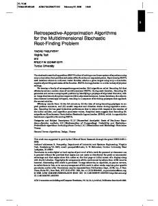
Figure 1: Counterexample for the simplest milling strategy. tool as a collection of simple regions of regular structure. If desired, the actual milling paths can be extracted by contour-parallel milling or zig-zagging within each output regions. We also output the cost of our approximate milling plan.
Outline of paper. Section 2 gives an overview of our approximation algorithms and states the main result. In Section 3 and 4, we show how to discretize the problem. Section 5 shows that our discretization method indeed approximates the milling problem to within a constant factor. Section 6 shows how to reduce the milling problem to a weighted set cover problem and describes the approximation algorithm.
2 Overview and summary of results Before discussing our approximation algorithm, we begin with some discussion to motivate the various elements of our solution. Since large tools can mill more material per unit of motion than small tools, the simplest strategy that comes to mind is to mill everything that can be reached by the largest tool, and then repeatedly load successively smaller tools and mill everything that is reachable for each tool. However, it is easy to see that this simple strategy may be suboptimal by a factor that is as large as the number of di�erent tools. For example, for the domain shown in Fig. 1, after the large tool has acted, all that remains are the small protrusions. The next smaller tool may only be able to shave away a small amount of additional material. The best option is to load a much smaller tool that can completely t within each of the small protrusions. The tradeo� that must be faced is whether to use a larger tool and mill potentially less material with greater e�ciency, or to use a smaller tool and mill more material with lesser e�ciency. At a very abstract level, milling the domain is equivalent to covering the points in the domain with copies of the tools available. Each copy of a tool used will incur some cost. This cost includes the time to load the tool, the time to mill the various regions, and the time to transport the tool from one unmilled region to the next. This suggests that milling is related to the discrete optimization problem of weighted set-cover (cover a domain by sets, each having an associated cost, so that the sum of costs is minimized). A well-known heuristic for weighted set-cover is the greedy algorithm [Chv79], which at each stage selects the subset that maximizes the number of items covered per unit cost. This algorithm is known to produce a logarithmic approximation ratio. We will transform the multiple-tool milling problem into a weighted set-cover problem and then solve the weighted set-cover problem by a greedy heuristic. 4
To construct the transformation, we need to de ne the elements in the base set and the weighted subsets. The transformation is not straightforward for two reasons. First, it is infeasible to use points as set elements directly as there is an in nite number of them. We overcome this by discretizing the domain into simple regions and use these simple regions as set elements instead. We will show how to construct this discretization such that we may assume that each simple region is milled with only one tool, while increasing the approximation ratio only by a constant. This is given in Sections 4 and 5. Each subset in our transformation will correspond to a milling action, which consists of loading a tool and then milling some subset of the remaining unmilled regions with this tool. The second problem is that it is not e�cient to enumerate the exponential number of possible subsets of unmilled regions in order to select the next subset. We overcome this by using an approximate greedy strategy that does not require the weighted subsets to be explicitly provided. This strategy will incur another constant factor in the approximation ratio, and it is based on the Euclidean k-TSP problem [Aro97]. (Here k is not the same as the number of tools.) It will be described in Section 6. Our discretization of milling actions is based on a subdivision of the milling domain P. We rst subdivide the boundary of P through the introduction of new vertices into O(n) segments, in order to satisfy certain monotonicity conditions, which will be described later. Let P � denote the modi ed domain. The size of our discretization is equal to the simple cover complexity of P �. The simple cover complexity, or scc(P � ), is an intrinsic measure of the geometric complexity of P � [MMS94]. It is de ned as follows. A disk is simple if it intersects at most 2 edges of P �. Given any � > 0, we say that a ball of radius r is �-strongly simple if the ball with the same center and radius (1+�)r is simple. Given �, a strongly simple cover of a region P � is a collection of �-strongly simple balls whose union contains P � . Given any xed � (for example � = 1=2), the simple cover complexity of P � is de ned to be the cardinality of the smallest strongly simple cover of P �. Our main result is:
Theorem 2.1 Given a domain P of n vertices, and k circular tools, let N = scc(P � ) denote the simple cover complexity of P �. Let �, , and , be nonnegative cost parameters (where � �). Then an O(log(kN))-factor approximation to the optimum cost milling plan for P can be computed in time that is polynomial in n, N and k. (Constant factors hidden by the \big-Oh" do not depend on any of the input parameters.)
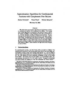
3 Subdividing the domain Let @P denote the boundary of the domain. Consider the Voronoi diagram of @P. We de ne a distance function v(p) which maps every point p on the Voronoi diagram to its closest point on @P. Consider the set of points p on the Voronoi diagram such that v(p) is locally minimal, in the sense that in every su�ciently small neighborhood of p there is a point on the Voronoi diagram with strictly higher distance value, and no point in the neighborhood has a strictly smaller distance value. For each such point p on the Voronoi diagram, the two nearest points on @P to p are called bottleneck points, and the line segment joining these boundary points is a bottleneck segment. (See Fig. 2 for example.) We introduce 5
Figure 2: The dotted curve shows the Voronoi diagram of the domain. White points are the bottleneck points and dashed segments are the bottleneck segments. all the bottleneck points as new vertices on the boundary of P. Each bottleneck point splits a domain edge into two smaller domain edges. We denote by P � the resulting domain. We will perform a quadtree decomposition of P �. This decomposition will subdivide the plane into a collection of square regions called boxes. For any box x, we denote its side length by width (x). For any positive real c, we denote by cx a box with the same center as x whose side length is c � width (x). The goal of the decomposition is to cover P � with a set X of boxes such that the portion of the domain lying within and near each box is extremely simple. X is generated as follows. We rst enclose P � in a bounding box. Then we apply the following splitting rule. For any box x, we call 3x the bu�er zone of x and denote it by buf (x). Take any box x, if buf (x) intersects more than two domain edges, then split x through its center into four identical boxes each of half the size. When the splitting process stops (which will occur eventually since each vertex is adjacent to at most two domain edges), we obtain a set of boxes covering P � . A cell is a connected component of P � \ x for some box x 2 X. Given a cell C, we denote by box (C) the box x 2 X that contains C. We de ne the size of C, size (C), to be width (box (C)). We de ne buf (C) to be buf (box (C)). The size of our subdivision of P � is bounded by the simple cover complexity [MMS94]. Such a quantity has been reported to be close to linear for practical scenes [dBKvdSV97], though hypothetical examples exist for which the simple cover complexity becomes unbounded. Lemma 3.1 There are O(scc(P � )) boxes covering P � . Proof To prove that jX j is O(scc(P �)) we consider an expansion factor of � = 1=2. As shown in [MMS94], the choice of � only a�ects the constant factor involved. Consider a strongly simple disk of radius r. This means that its expansion by a factor of 1 + � = 3=2 does not intersect more than two edges of P � . We claim p that any box in X that overlaps the (unexpanded) disk has width that there is a box x which overlaps � r=(12 2). Suppose to the contrary p the diskp and has width < r=(12 2). Then the parent p box p of x has width < r=(6 2). Thus, buf (p) has width at most r=(2 2) and hence a diameter of at most r=2. Thus buf (p) lies entirely within the expanded disk and so intersects at most two edges of P � . Consequently p cannot be split further. 6
t
Figure 3: The accessibility arcs for tool t. This is a contradiction. It follows thatpany strongly simple disk cannot contain a box of X of width less than r=(12 2). By a simple packing argument, it follows that the number of boxes in X that overlap any strongly simple disk is a constant. Since the simple disks cover P � , it follows that jX j is bounded by a constant factor times the number of simple disks, and hence is O(scc(P � )). ut
4 Basic milling actions As mentioned above, our approximation algorithm is based on discretizing the space of possible milling actions into what we call basic milling actions, or BMAs for short. Each basic milling action is responsible for milling a certain portion of the domain by a single tool. In general, many tools may be able to access a given region, and the de nition of BMA makes no attempt to limit which tool is responsible for some region. It will be the responsibility of the greedy algorithm, described in Section 6, to determine which BMAs to apply to employ for the nal plan. We begin by introducing some notation. Let d(p; r) denote a disk of radius r centered at a point p. Given a tool t, we also use t to denote its radius. Whenever we put the center of t at a point p, we call d(p; t) a placement of t. A placement of t is free if it lies within P �. The free space of t is the locus of centers of all free placements of t. We denote it by F (t). Formally, F (t) = P � t, where is the Minkowski di�erence operator. Thus, F (t) � t is the set of points in P � that can be covered by a free placement of t, where � is the Minkowski sum operator. At each vertex p of F (t), d(p; t) touches @P � at several points. If the arc � between two consecutive contact points on the boundary of d(p; t) is less than a semicircle, then we call it an accessibility arc. The collection of accessibility arcs for a tool t is denoted by A(t). See Fig. 3. A subset K of F (t) and a subset M � K � t de ne a milling action. Speci cally, t moves with center in K to remove all points in M. If K is not connected, then we have to pick t up transport it to another component and place it. This will incur a charge of 2t per connected component in K plus the transport cost to visit all components in K. We say that a point in M is milled by this action. Note that, physically speaking, a larger set than M may be removed by t's movement. However, we only consider points in M as milled, and we will have 7
to deploy other milling actions to mill points not in M. Imagine that an arbitrary sequence of milling actions (possibly of di�erent tools) has been applied to the collection of cells de ned in the previous section. Given a cell C, we call the set of points in C not milled the unmilled region, and we call a connected component of the unmilled region an unmilled component. Given a tool t, we restrict ourselves to two kinds of milling actions of t on a cell C, depending on the relative sizes of t and C. We say that t is large for a cell C if t � size (C)=16 and small if t � size (C)=4. Conversely, we say that a cell C is small for t if t � size (C)=16 and large if t � size (C)=4. Note that this implies that in the range size (C)=16 � t � size(C)=4, t is both small and large for cell C. In the next two subsections we describe the basic milling actions for large tools and small tools.
4.1 Large-tool basic milling action
Recall that the goal of de ning basic milling actions is to provide a discretization within which to approximate any milling action. Since we do not know the optimum milling path for any tool, our approach will be to de ne each largetool basic milling action to mill a local region whose size is proportional to the size of the milling tool. Then we will be able to approximate the milling action of any milling plan by concatenating a sequence of such local milling operations. Since basic milling actions are de ned independently of one another, we cannot generally predict whether a given milling action will simply be a continuation of a neighboring milling operation, or whether it will require placing the tool of size t into the material. Recall that each such placement incurs a cost of 2t by our model. To absorb this potential placement cost, we de ne each basic milling operation (except for the smallest tool) so that there is a free placement of a tool of twice this size. This insures that there will be su�cient millable area, so that placement costs will not dominate milling costs. One of the tricky issues in de ning basic milling actions for large tools is that a single large tool may mill portions of many small cells at the same time. Thus, if we were to account for the milling cost on a cell-by-cell basis and sum these costs, then we may considerably overestimate the actual milling cost. In order to accurately account for the total cost of using a large tool to mill many smaller cells, it is important to de ne the milling actions for large tools in a way that is global to the small cells that it a�ects. We do this by overlaying a grid on the domain whose side length is proportional to the tool size, and then associating each basic milling action with each grid cell. A second issue is predicting the possible shapes of the unmilled regions that result after each basic milling action. To minimize the number of possibilities, our milling actions are de ned so that if a cell cannot be milled entirely, then we mill up to an accessibility arc for this tool. Overlay a square grid Gt of side length t on P �. De ne Bt to be the set of grid squares b such that b � 4t overlaps some quadtree box of width less than 16t. Any grid square b 2 Bt induces a (possibly empty) set of milling actions as follows. If t is the smallest tool, let K be a connected component of (b � 28t) \ F (t); otherwise, let K be a connected component of (b � 28t) \ F (t) that contains some component of b \F (2t). De ne Cb to be the collection of cells S C such that t is large for C and C overlaps b � 4t. De ne M to be K � t \ C 2Cb C. Then K and M de ne a large-tool basic milling action denoted by large tool (t; K; M), 8
t
16t
0 on s. If C 0 does not encounter any other domain boundary point not on s for some �, then after the sliding, we can expand C 0 slightly while maintaining emptiness. This shows that xy is a bottleneck segment. Suppose that for all � > 0, C 0 will encounter some domain boundary point not on s. The rst possibility is that C touches another domain boundary point z on the semi-circle to the left of xy, but this means that xz or yz is shorter than xy, contradiction. The second and last possibility is that during the sliding, C 0 always touches or contains some point on the domain edge containing y. But this contradicts either the shortestness or the leftmostness of xy. Hence, we conlude that xy is a bottleneck segment intersecting pq. Now, suppose to the contrary that three disks of D0 centered at some points p, q, and r have pairwise nonempty intersection. We will show that for all su�ciently small values of c, this will imply that F (t) is not connected, leading to a contradiction. (See Fig. 6(b).) From the observations of the previous paragraph, it follows that there are bottleneck segments that intersect each 12
r p
q
p
q
(a)
(b)
Figure 6: Bounding the number of connected components. The solid circles have radius t, dashed circles have radius t0 , and dotted lines are bottleneck segments. edge of the triangle pqr. Hence, there is a point, say p, that lies between the bottleneck segments s1 and s2 that intersect pq and qr. Also, s1 and s2 intersect a disk of radius 2t0 centered at p. Consider the quadrilateral de ned by the endpoints of s1 and s2 (which may degenerate to a triangle if s1 and s2 share a common endpoint). Observe that as the parameter c decreases, s1 and s2 intersect a shrinking disk centered at p with p lying between them. Since the lengths of s1 and s2 are less than 2t, and it passes arbitrarily close to the center of p its length approaches 2t as c approaches zero. Since s1 and s2 do not intersect, the other two sides of the quadrilateral will fall below any given threshold for su�ciently small c. At the same time, p will lie inside the quadrilateral. Thus there exists a constant value of c so that all four sides of the quadrilateral are of length less than 2t. Since p lies inside the quadrilateral whose vertices are points of P's boundary and whose sides are shorter than 2t, the placement of t at p is e�ectively trapped at this location. In particular, the connected component of F (t) containing p has a diameter less than t, and hence lies entirely within b � 2t. However, because q and r are in di�erent connected components of b � 2t \F (t), they are in di�erent connected components of F (t). This contradicts the hypothesis that F (t) is connected. ut
Lemma 4.6 There are O(1) large-tool BMAs for t induced by any grid square
b 2 Bt .
Proof If t is the smallest tool, let K be the set of connected components of b � 28t \ F (t) that overlap b � 4t. Otherwise let K be the set of connected components of b � 28t \ F (t) that contain some component of b \ F (2t). Since one large-tool BMA for tool t is de ned for each component in K, it su�ces to show that the number of components in K is O(1). Consider the case when t is not the smallest tool. Let K be any component in K. Since K contains a component of b \F (2t), there is a free placement d(p; 2t) where p 2 K \ b. Clearly d(p; t) � F (t) since a disk of radius t with center in d(p; t) lies completely within d(p; 2t). Further, since p 2 b, d(p; t) � b � 28t. It follows that d(p; t) � K. By a packing argument, the number of components in K is O(1). 13
If t is the smallest tool, then by our assumption F (t) is one connected component. Since b is of side length t, we can cover b � 4t with a constant number of boxes of side length t. Let b0 be any such box. Since (b0 � 2t) � (b � 28t), the number of connected components of b � 28t \ F (t) that overlap b0 is not greater than the number of connected components of b0 � 2t \ F (t) that overlap b0 (since expanding the region can only improve connectivity). Thus, by applying Lemma 4.5 to b0, it follows that this number of connected components is O(1). This implies that the number of components in K that overlap b � 4t is O(1). ut
Corollary 4.1 There are O(kN) large-tool BMAs for all tools. Proof For each tool t, we de ne large-tool BMAs for each b 2 Bt . Since a quadtree box of width less than 16t can overlap b � 4t for at most a constant number of grid squares b in Gt, the number of squares in Bt is O(N). By Lemma 4.6, the number of large-tool BMAs induced by each b 2 Bt is O(1). It follows that there are O(N) large-tool BMAs de ned for a given tool t. Summing over all tools, we have the desired result. ut
4.2 Small-tool basic milling action
Unlike the large-tool BMAs, small-tool BMAs only act on a single cell of the subdivision. At some stage when a small tool rst acts on a cell, other tools may have already milled portions of this cell, leaving one or more unmilled regions. We do not know what these tools are, but (as we have already seen with the large-tool BMAs) we design each BMA so that it either mills the entire region or it mills up to an accessibility arc. Henceforth, the term unmilled component will refer to an unmilled component that could have resulted by any sequence of BMAs. (Later we will show that no matter what combination of tools have acted on this cell, the number of possible unmilled components that could result is polynomially bounded.) Intuitively, the task of each small-tool BMA is to mill as much material as it can access within an unmilled component such that the tool is always in contact with the unmilled component. Let U be an unmilled component of C such that t is small for C. Let K be a connected component of U � t \ F (t). De ne M to be K � t \ U. K and M de ne a small-tool BMA by t, denoted small tool (t; K; M). This action will move t on the surface with center in K to mill points in M. As in the large-tool case, we will prove that the unmilled components remaining after a small-tool BMA will be bounded by the boundary of the cell and portions of accessibility arcs. In fact, we will show that for small-tool BMAs, each unmilled component is bounded by at most one accessibility arc. From this we will show that each unmilled component has constant combinatorial complexity.
Lemma 4.7 After small tool (t; K; M) acts on an unmilled component U in a cell C , any resulting unmilled component is bounded by a portion of at least one accessibility arc of radius t. 14
t F (t )
K U
Figure 7: Small-tool BMA. U is bounded by the domain boundary and solid lines. F (t) is shown with dashed lines, and K is shown with dotted lines. All of U is milled except the portion below the accessibility arc at the bottom.
Proof Let W be a resulting unmilled component. Take a point q in @W n @U.
Such a point q must exist, otherwise U was not a�ected by small tool (t; K; M). By our choice, q is milled by small tool (t; K; M) and there is a free placement d(p; t) that touches q, where p 2 K. We claim that p must lie on the boundary of F (t) and so q 2 A(t) or q 2 @P � . The latter is impossible as q 2 @C otherwise. Assume to the contrary that p lies in int (F (t)). If p lies on the boundary of U � t, then q 2 @U which is impossible. The other possibility is that p lies in the interior of a connected component of U � t \ F (t) which is a subset of K. This implies that p 2 int (K) and we can perturb p to another p0 2 K such that d(p0; t) contains a small neighborhood of q. Thus a small neighborhood of q should have been milled which contradicts that q 2 @W n @U. ut Next, we strengthen our result and show that each resulting unmilled component is bounded by exactly one accessibility arc of A(t). To this end, we need two technical results Lemma 4.8 and Corollary 4.2. They are illustrated in Fig. 8. Let us think of each edge of P � as being an open curve (line segment or circular arc). Observe that when an accessibility arc of some tool t is incident to an edge of P �, the point of incidence subdivides this edge into two portions. Locally about the point of incidence, one portion contains points that are accessible to t and the other contains points that are not. Points that are not accessible to t are said to lie outside the accessibility arc. Observe that unmilled regions are always locally outside of any accessibility arcs on their boundaries. Two accessibility arcs that are incident to the same edge are said to face each other if the points between these accessibility arcs lie outside of both arcs. We show that, because of the introduction of bottleneck points, it is not possible for two facing accessibility arcs to be incident to the same edge of P �. Lemma 4.8 If the interior of an edge of P � is incident to an accessibility arc for tool t, then no point on the outside portion of the edge is accessible to t. Proof Assume to the contrary that a domain edge e is incident at a point q1 to an accessibility arc of radius t and that there a free placement of t that intersects a point of e that is outside this arc. (See Fig. 8(a).) Consider the point of contact q2 of such a placement that is closest to q1 . Clearly the placement must 15
t
t
e
q1
q2
?
t
t
e
q1
(a)
?
q2
(b)
Figure 8: Facing accessibility arcs. be tangential to e at this point. Since the placement cannot be moved closer to q1, there must be a second accessibility arc incident to e at q2 such that both accessibility arcs face each other. Because these accessibility arcs are blocked by some other boundary points, it follows that their centers lie on the Voronoi diagram of P �. The Voronoi distance function v(p) is equal to these t at each center and is smaller in between (for otherwise there would be a free placement of t that is closer to q1 along e). Therefore, there must be a bottleneck point somewhere within the segment q1q2, contradicting the hypothesis that they both lie on the same edge of P � . ut
Corollary 4.2 An edge of P � cannot be incident to two accessibility arcs (of possibly di�erent sized tools) that face one another.
Proof If two such arcs exist, then the arc with a larger radius can accommodate a disk that has the same radius as the other arc and touches the domain edge. (See Fig. 8(b).) This contradicts Lemma 4.8. ut Lemma 4.9 Each unmilled component W resulting after the action small tool (t; K; M) is bounded by points belonging either to @C or to exactly one accessibility arc of A(t). Proof
By Lemma 4.7, @W contains a portion of some accessibility arcs of radius t. Since t is small for C, the contact points between � and P � are within buf (C). Recall that there can be at most two edges of P � within buf (C). First we observe that both endpoints of � cannot lie on the same domain edge. This is a simple consequence of the facts that � is a circular arc subtending an angle less than �, the domain edges are either straight line segments or circular arcs, and that buf (C) intersects at most two edges of P � . Let e1 and e2 denote the two domain edges to which � is incident. We assert that each edge is tangentially incident to �. If not, then one endpoint of � must coincide with a vertex of P � , and the other with one of the edges e1 or e2 . However, either this vertex is incident to a third edge (contradicting the fact that buf (C) can intersect at most two edges) or else both endpoints of � are incident to a single edge (contradicting the previous observation). Consider the subregion R of box (C) bounded by � and e1 and e2 (See Fig. 9(a)). W lies within R. Suppose that W was bounded by some other accessibility arc . Since unmilled regions lie outside of their accessibility boundaries, 16
dβ R
β
e2
e1
e2
e1 α
α
dα
dα
(a)
(b)
Figure 9: Bounding the combinatorial complexity of unmilled regions for smalltool BMAs. � and face one another. If has radius no greater than �'s, then was also produced by a small milling action. By applying the above analysis it follows that is incident to e1 and e2 . However, the existence of an edge incident to two accessibility arcs that face one another contradicts Corollary 4.2. Otherwise, if 's radius is greater than �'s, then there is a free placement of a disk d of radius t that intersects R and lies on the inside of . (See Fig. 9(b).) If we move d towards the disk d� the fact that � is an accessibility arcs implies that d must contact the domain boundary at some point. This contact must be with either e1 or e2 , by the same analysis used above for �. However, this free placement along such an edge contradicts Lemma 4.8. Hence, we conclude that W is bounded by only one accessibility arc of radius t.
ut
4.3 Complexity of unmilled region
In this section, we establish that after any sequence of BMAs the combinatorial complexity of the unmilled region inside a cell is always bounded by a constant. In the sequence, tools can change and large-tool and small-tool BMAs can interleave. The consequence is that within each cell, the number of unmilled components is always bounded by a constant and each unmilled component has constant complexity.
Lemma 4.10 After any sequence of BMAs on a cell C , the unmilled region in C has constant combinatorial complexity.
Proof
The proof involves two cases, depending on whether the unmilled component resulted from a small-tool or large-tool basic milling action.
Small-tool Case. By Lemma 4.9, after a small-tool BMA, each unmilled component of C is bounded by straight line segments and circular arcs, limited 17
to the four sides of box (C), at most two domain edges of P � , and at most one accessibility arc. Therefore, each unmilled component has constant combinatorial complexity. Thus, it su�ces to show that the number of connected components is bounded. Moreover, we assert that each unmilled component U either borders a domain edge intersecting C or a vertex of box (C). To prove this, observe that if U is not bounded by @P � , then for any maximal connected component s of a side of box (C) bounding U, s lies outside of at most one accessibility arc by Lemma 4.9. Thus, the other endpoint of s must be incident to a vertex of box (C). Since there are only a constant number of box vertices, it su�ces to show that the number of connected components bounded by domain edges is bounded. Each domain edge intersecting C cannot border more than two unmilled components, for otherwise the domain edge would be incident to two accessibility arcs that face each other, contradicting Corollary 4.2. (The worst case occurs when both of the edge's vertices lie within unmilled components, and hence each faces an accessibility arc.) Therefore, the total complexity of all unmilled components produced by small-tool BMAs acting on C is a constant.
Large-tool Case. Let U denote the set of unmilled components of C that
resulted from large-tool milling actions. We assert that no component of U can be bounded by the accessibility arc of a tool smaller than size (C)=16. This is because such an arc would have resulted from the milling action of a small-tool BMA. By de nition such a milling action it would remove everthing reachable to this tool within the component. This implies that no larger tool could later introduce an accessibility arc into the remaining unmilled component. Thus, it su�ces to bound the number of accessibility arcs of radius at least size (C)=16. p To simplify the analysis, we overlay a square grid on C of side length 2r, where r = size (C)=32. The number of such boxes is bounded by a constant. Consider one such box x. Observe that if we enclose x within a disk Dr of radius r, then the closest point outside buf (C) is at distance greater than r from Dr . We will show that the number of accessibility arcs for all large tools t that may contribute to the intersection of @U with Dr is O(1). It will follow that the number of accessibility arcs that bound the U is also O(1). Let c be the center of Dr . Let D2r be a disk of radius 2r centered at c. Since D2r lies entirely within buf (C), at most two edges of P � may intersect this disk. (See Fig. 10(a).) Let fdi g be the set of free placements of tools for C that support accessibility arcs that contribute to the intersection of @U with Dr . Let fcig be their respective centers. The radii of each disk is at least size (C)=16 � 2r. Sort these disks in angular order about c according to locations of their centers. If there are no three consecutive disks d1 , d2 , and d3 such that \c1cc2 < �=6 and \c2 cc3 < �=6, then it follows that there are at most 24 such disks (two per each sector of �=6). We will show that if we exceed this number by more than a small additive constant, then there will be a triple of consecutive disks, d1, d2 , and d3, satisfying this condition, such that one of these three disks is free to move further into Dr . However, this will imply that it could not contribute an accessibility arc, a contradiction. First, by simple trigonometry, any disk di of radius at least 2r that intersects Dr must intersect D2r along an arc of angle at least 2 arccos(3=4) � 1:445 > �=3. 18
D
D
2r
c
2r
Dr
Dr
c
p
d1
c3
c1
d3
c3
c2
d3
q c2
d2
(a)
(b)
Figure 10: Bounding the combinatorial complexity of unmilled regions for largetool BMAs. Second, if we draw a diameter of di perpendicular to cci (shown as a dashed line between shaded points in Fig. 10(a)), and join c to one diameter endpoint and ci , then the angle between these rays is at least arctan(2=3) � 0:588 > �=6. (In both cases, the minimum occurs when di has radius exactly 2r, and ci is at distance 3r from c.) Third, the center of no di can lie inside D2r , otherwise, di would completely enclose Dr , implying that di contributes no accessibility arc that intersects Dr . We consider two possible con gurations of d1, d2 , and d3 depending on the position of the endpoints of the diameter of d2 perpendicular to cc2. Call this diameter l2 (the dashed line segment in Fig. 10(a)). In the rst case, both the endpoints of l2 lie inside d1 and d3 . By the lower bound on the radii of d1 and d3 and the upper bound on the angle their centers subtend about c, it follows that l2 is fully contained within the union of d1 and d3. Since these are both free placements, and since d2 contributes an accessibility arc, it follows that d2 must contact @P � along the portion of the arc of d2 that lies within D2r n (d1 [ d3 ). By the same reasoning used in Lemma 4.9, it follows that this accessibility arc must contact both of the domain edges of P � that lie within D2r . However, observe that d2 is unique in this, since no other accessibility arc can have its contact points lying on the edges of P � within D2r without violating Corollary 4.2. Thus excluding d2, no other accessibility arc can be in this con guration. For the second con guration, either the left endpoint of l2 lies outside d1 or the right endpoint of l2 outside d3. Let us consider the latter, as the other case is symmetrical. (See Fig. 10(b).) Let l3 be the diameter of d3 that lies on the line through c and c3 (shown as a dotted line in the gure). From the trigonometric observations above it follows that l3 lies within D2r [ d2 . If the portion of @d3 that contributes the accessibility arc intersects the domain boundary within D2r , then this contact involves one of the two edges of @P � that lies within D2r . Again, by 4.2, this can only happen for a constant number of accessibility arcs. Otherwise, the closest contact of d3 with the domain boundary occurs at some point p that lies outside D2r . The point q on @d3 that is diametrically opposite 19
to p, lies in d2. However, the arc of length � from q to p is free from contact with the domain boundary, contradicting the hypothesis that d3 contributes an accessibility arc. ut
Lemma 4.11 Given an unmilled component U in a cell C and a tool t small for C , U � t \ F (t) consists of a constant number of components, each of constant combinatorial complexity.
Proof Let x be 23 box (C). If t moves with center in x, then t is entirely inside buf (C). Since there are at most two domain edges intersecting buf (C), the complexity of x \ F (t) is bounded by a constant. By Lemma 4.10, the complexity of U is bounded by a constant. Since U � C and t is small for C, U � t � x. So U � t \ F (t) = U � t \ (x \ F (t)) which is the intersection of two shapes of constant combinatorial complexities. Thus, we conclude that U � t \ F (t) consists of a constant number of components, each of constant combinatorial complexity. ut Lemma 4.12 There are O(N(kn)O(1)) basic milling actions by small tools. Proof It su�ces to prove that there are O((kn)O(1) ) basic milling actions by
small tools in a cell C. By Lemma 4.1, Lemma 4.9, and Lemma 4.10, after any sequence of BMAs the boundary of the unmilled region in C is bounded by at most a constant c elements of the following varieties: line segments on the boundary of box (C), the at most two domain edges intersecting box (C), and accessibility arcs. There are k di�erent tools and there are O(n) accessibility arcs for each tool size. Therefore, there are O(kc nc) possible unmilled regions which may be generated after some sequence of milling actions. Hence, there are O(kc nc ) unmilled components that a basic milling action by a small tool t (with respect to C) may act on. Given an unmilled component U, U � t \ F (t) consists of a constant number of components by Lemma 4.11. This gives rise to a constant number of basic milling actions by t on U. In all, there are at most O(kc+1 nc ) basic milling actions by some small tool in C. Summing over all cells, we obtain the bound O(kc+1 nc N). ut
5 Approximating optimal milling using BMAs The main result of this section is to show that any milling plan can be converted into a milling plan consisting entirely of BMAs while sacri cing at most a constant factor in cost. We associate with each BMA large tool (t; K; M) or small tool (t; K; M) a starting point, which may be any point in K. When we perform a BMA, the tool will rst be placed at the starting point and at the end, the tool is returned to this point. De ne mill (t; K; M) to be the milling cost of the milling operation de ned by the BMA large tool (t; K; M) or small tool (t; K; M). Given a set of BMAs S, de ne St to be the subset of S which uses tool t. De ne TSP (S) to be the 20
length of a minimum Euclidean traveling salesman tour on the starting points of S and the tool-change center. The cost of S is composed of two elements: the time required to perform each of its milling operations and the time to move from the starting point of one to the starting point of another. De ne mill (S) to be the sum of mill (t; K; M) P for all large tool (t; K; M) and small tool (t; K; M) in S. De ne transport (S) = t TSP (St ). We immediately have the following.
Lemma 5.1 Let S be a set of BMAs which mills P � . Then there exists a
milling plan , using tools in S , such that mill ( ) = mill (S);
transport ( ) = transport (S):
Conversely we assert that any milling plan can be transformed into a set of BMAs which mills P �, whose milling and moving times are comparable to those of . Before proving this main result, we prove three technical lemmas.
Lemma 5.2 Consider any path of length L among a uniform rectangular grid of side length s, and let m be the number of cells ofpthe grid that the path intersects. Then there is a constant c (which is at most 2 2) such that m � cL=s + 4. Proof Replace the path by a rectilinear path by breaking it at its intersection p points with the grid. The resulting path is longer by a factor of at most 2. In the worst case, the path starts very close to a vertex, and so it can visit four cells within an arbitrarily small distance. After this, with each walk along the path by distance s the path can visit p at most two new cells. Thus the numberut of cells visited satis es m ? 4 � 2 (2)L=s. Lemma 5.3 For any path � of length L, there is a sequence S of disks d(pi; 2t), where 1 � i � dL=te and pi lies on �, such that � � t � i d(pi; 2t).
Proof Put d(p1; 2t) at an endpoint p1 of �. Traverse � from p1 to the other
endpoint. When � leaves d(p1; t) for the rst time, put d(p2; 2t) at the exit point. Repeat the above until we reach the other endpoint of �. The result follows by observing that each placement is separated by an arc length of at least t. ut
Lemma 5.4 Let C1 and C2 be two cells such that size (C1) � size (C2). If (box (C1)�t)\(box (C2)�t) is nonempty for some t � size (C1)=3, then size (C2) � size (C1)=100. Hence, for any point q, there are O(1) cells C such that box (C) � (size (C)=3) contains q.
Proof Assume to the contrary that size (C2) < size (C1 )=100. Since t � size (C1)=3 and (box (C1) � t) \ (box (C2 ) � t) is nonempty, both the horizon-
tal and the vertical distances between the centers of box (C1) and box (C2) is less than 7size (C1 )=6+ size (C2)=2 < 1:4size (C1 ). The bu�er zone of the parent of box (C2 ) lies inside 9box (C2 ) and has width at most 0:09size (C1). Thus, the bu�er zone of the parent of box (C2) lies inside 3box (C1) which is the bu�er zone of box (C1). This implies that the bu�er zone of the parent of box (C2 ) intersects 21
at most two domain edges, which contradicts the splitting of it. Therefore, we conclude that size (C2 ) � size (C1 )=100. Take any point q. Let C be the cell of the largest size such that q 2 box (C) � (size (C)=3). Thus, a square of width 3size (C) centered at q contains all the boxes box (C 0) for some cells C 0 such that q 2 box (C 0 ) � (size (C 0 )=3). From the above size (C 0) = �(size (C)). So a packing argument shows that there are O(1) of such boxes. Since each cell is a connected component of a box and each box intersects at most a constant number of domain edges, the number of cells is also O(1). ut
Theorem 5.1 Let be a milling plan. Then there exists a set S of BMAs which mills P � using at most twice the number of tools as in , such that mill (S) = O(mill ( )) and transport (S) = O(mill ( ) + transport ( )). The proof of this theorem is presented in the remainder of this section. We rst identify a set S1 of large-tool BMAs and then a set S2 of small-tool BMAs that mills P �. Clearly, mill (S1 [ S2 ) = mill (S1 ) + mill (S2 ) and transport (S1 [ S2 ) � transport (S1 ) + transport (S2 ). Thus, it su�ces to bound the milling and transport costs of S1 and S2 separately by mill ( ) and transport ( ). Each of S1 and S2 will involve at most the same number of tools used in . Thus ntools (S1 [ S2 ) � 2ntools ( ). For each tool t, t denotes the set of milling paths involving t, and �t denotes the set of milling paths involving t or smaller tools. We think of t as the set of paths along which the center of the tool moves and the same applies for �t. To complete the proof, we present the analyses of the large-tool and small-tool cases in the next two subsections.
5.1 Large-Tool BMAs
For each continuous curve �t in t , we nd a set of large-tool BMAs so that if a point q in a cell of size less than 4t is milled by t traversing along �t, then q is milled by some large-tool BMA in this set. Let t0 be the smallest tool in the range (t=4; t]. Let Xt be the squares b in the grid Gt through which �t passes. For each square b 2 Xt , we add to S1 all large-tool BMAs large tool (t0; K; M) induced by b such that K contains a point on �t inside b. We claim the following: (1) If a point q in some cell C is milled by a tool in of size greater than size (C)=4, then q is milled by a large-tool BMA in S1 . (2) mill (S1 ) = O(mill ( )) and transport (S1 ) = O(mill ( ) + transport ( )). To prove (1), since q is milled by some tool t of size greater than size (C), q 2 d(p; t) for some point p on a curve �t in t . Let b be the square in Gt that contains p. Let K be the connected component of (b � 28t0) \F (t0) that contains p. (Note that K must exist as b � 28t0 contains p and F (t) � F (t0 ).) We claim that b induces the BMA large tool (t0 ; K; M) which is added to S1 . Since p 2 b and d(p; t) overlaps C and t < 4t0, this implies that b � 4t0 overlaps C. Also, since size(C) < 4t and t < 4t0, size(C) < 16t0. If t0 is the smallest tool, then we are done. Otherwise, we need to check if K contains a component of b \ F (2t0). Since t � 2t0 by choice of t0 , F (t) � F (2t0). Since p 2 F (t) and p 2 K, we conclude that K contains a component of b \ F (2t0). Finally, we verify that 0
0
0
0
22
large tool (t0; K; M) mills q. Recall that q 2 d(p; t) for some p on �t and p 2 K.
Thus, one can rst center t0 at p and then move within d(p; t) to mill q. To prove (2), by Lemma 5.2, each �t in t passes through O(L�t =t + 1) squares in Gt and so Xt has O(L�t =t + 1) squares. By Lemma 4.6, each square in Xt induces O(1) large-tool BMAs for t0. So the total number of large-tool BMAs identi ed for �t is O(L�t =t + 1). By Lemma 4.4, the total milling cost of these BMAs is O(t0 (L�t =t) + t0) = O(L�t + t0) which is bounded by the milling cost of �t (length plus placement cost 2t). Thus summing over t for all t, we have mill (S1 ) = O(mill ( )). We can visit all the large-tool BMAs in S1 involving tool t as follows. Follow to transport t to a point on �t. Then transport t to an endpoint of �t (this costs O(L�t ). Transport to the starting points of the large-tool BMAs de ned at this endpoint and apply the BMAs. Traverse along �t to the center of the next disk in D�t and repeat the application of BMAs (this costs O(L�t + t)). Finally, transport t to the point on �t from where will leave �t (this costs O(L�t )). Thus, the entire tour can be viewed as the transport of t in plus some detour. The cost of the detour sums to O(mill ( t )). Thus, transport (S1 ) = O(mill ( ) + transport ( )). 0
0
0
5.2 Small-Tool BMAs
We assume that all the large-tool BMAs in S1 have been applied. Let C be a cell with an unmilled region. Any tool t in that acts on this unmilled region must satisfy t � size (C)=4 and so t must be small for C. We will identify a set S2 of small-tool BMAs to mill the rest of P � and charge the cost to mill ( ) and transport ( ). The charging scheme for the small-tool BMAs is more complex than for large tools. Consider some unmilled component. Let t be the largest tool used by to mill any point of this component. We will introduce the corresponding small-tool BMA for t to mill as much of this component as possible without losing contact with it. The key to establishing the approximation bound is to show that no combination of smaller tools could mill the same region with signi cantly less cost. Recall from Section 2 and Fig. 1 that one reason that larger tools are not necessarily better than smaller tools is that a large tool may only shave away a small amount of additional material, into which a small tool may be able to plunge deeply. Intuitively, if tool t does plunge deeply into the unmilled region, then it will mill more e�ciently than a smaller tool. On the other hand, if t does not plunge deeply into the unmilled region, then the smalltool BMA will scrape along the boundary of the unmilled region. To account for this, we will introduce a charging scheme to pay for this milling action. The boundary of each unmilled region will be assigned a charge proportional to its length. We will then show that the total charges will be dominated by the other costs of our milling plan. To facilitate the charging, we need to initialize some charge on boundaries of unmilled regions after applying all large-tool BMAs in S1 . For each segment on these boundaries, we associate a charge proportional to its length. We claim that these charges can be paid for by mill ( ) and the argument is as follows. By Lemma 4.2, the sum of lengths of segments that lie on accessibility arcs left by large-tool BMAs in S1 can already be paid for by mill (S1 ), which is O(mill ( )). The other boundary segments of the unmilled regions lie either on 23
the boundary of quadtree boxes or domain edges. Let s be a boundary segment of the unmilled region in a cell C that lies either on the boundary of box (C) or on some domain edge bounding C. Let t be the largest tool in that mills any point on s. Consider s � t. Suppose that s is a straight line segment. Let t0 be the tool traversing a subpath �t in \ s � (4t=3) such that �t � t0 overlaps s. Note that t0 � t. By we take all such than j�t j + O(t0). If P Lemma 5.3, the perimeter of �t � t0 is less S tools and subpaths, then s is covered by t �t � t0 and so jsj � t j�t j +O(t0). Notice that each �t either traverses a distance of at least t=3 in s � (4t=3) n (s � t) or contains a placement of t0 . Thus, the O(t0 ) term can be charged to this placement or �t itself. Thus, jsj can be charged to the total cost of such milling subpaths �t . Hence, by Lemma 5.4 and Lemma 4.10, the total length of straight line segments of the unmilled regions can be charged to O(mill ( )). The possibility that s is a circular arc can be handled identically. This proves our claim that charges associated with boundaries of unmilled regions after applying large-tool BMAs in S1 can be paid for by O(mill ( )). Let U be the set of unmilled components after applying large-tool BMAs in S1 . We de ne the set S2 of small-tool BMAs iteratively as follows. Remove U 2 U . Let t be the largest tool in that mills any point of U. For each connected component K of (U � t) \ F (t) that intersects t , we add small tool (t; K; M) to S2 . Then we subtract K � t from U for each such K and put the unmilled components produced back to U . We repeat the above until U becomes empty. We bound mill (S2 ) by bounding the placement costs and millingpath lengths separately. Take any small tool (t; K; M) 2 S2 . In t , there is either a placement of t in K � t or a segment � of length t in (K � t) n K. We charge the placement cost of small tool (t; K; M) to this placement in K � t or the length of �. At any moment in time, a point q on t can only lie inside K for at most a constant number of small-tool BMAs in S2 by Lemma 5.4, Lemma 4.10, and Lemma 4.11. Moreover, after applying small tool (t; K; M), q is at distance at least t away from any new unmilled component produced. Thus, q cannot be charged again for these new unmilled components or any subset of them. P Therefore, the placement costs of small-tool BMAs in S2 is bounded by O( t mill ( t )) = O(mill ( )). To bound the milling path length of small tool (t; K; M), consider the intersection ? = K \ �t . ? [ @K is an arrangement of curves (possibly consisting of several connected components). (See Fig. 11(a), for example.) For each tool t0 used in �t , we let �t denote the portion of a milling path for tool t0 that lies in ?. If we move t along @K and t0 along �t for each �t 2 ?, we must mill the entire K � t. The reason is as follows. Let q be any point in K � t. If q is at distance � t from some point on @K, then it must be milled as t is moved along @K. If q is at distance > t from every point on @K (i.e. q 2 K t), then q must lie inside U. Further, since t is the largest tool in that mills any point of U, q must be milled by using a tool t0 of size � t. Clearly, the center of such a tool t0 lies within K. Our plan is roughly to move t almost along ? [ @K to bound the milling path length of small tool (t; K; M). The main problem with this strategy is that if ? consists of many di�erent components, then the placement cost of t for each component cannot be paid for by the much smaller placement costs that may have been incurred by . To remedy this, we will add extra segments to connect all components in ? [ @K; we will show that the length of these segments can 0
0
0
0
0
0
0
0
0
0
0
0
24
0
0
K
K
(a)
K
(b)
(c)
Figure 11: Charging argument for small-tool BMAs. Figure (a) shows K \ �t . Figure (b) shows �� for one component � shown in bold. Figure (c) shows the trimmed �� for another component � shown in bold. be paid for either by the length of these components or by the placement costs in . Each connected component � of ? [ @K can be viewed as a single oriented curve by an Eulerian traversal. Let t� be the largest tool used in � (we assume that t is used for @K). By Lemma 5.3, we can nd L� =t� + 1 disks of radius 2t� to cover � � t� , where L� is the length of �. We add a straight line segment of length 2t� to connect the envelope of the union of these disks and �. We denote the union of this extra line segment, the boundaries of the disks and � collectively by �� . (For example, see Fig. 11(b).) The total length of �� is O(L� + t� ). Also, let �R denote the region formed by taking the union of these disks. If we could move t� along �� , then this would mill all of �R . However, it may not be possible to move t� along �� , if it projects outside of K. Therefore, we trim �R by taking its intersection with K. Also, we trim �� by taking its intersection with K and then adding the portion of K that lies within the (trimmed) �R . (For example, see Fig. 11(c).) We claim that moving t� along �� mills all of �R . For the sake of contradiction, assume that there is a point q in �R which cannot be milled by moving t� along �� . Let q be inside disk x. Then q cannot be within distance t� of center of disk x because moving t� along � would mill q and �� contains � since � lies entirely within K. Let p denote the closest point to q on the boundary of disk x. Clearly p must lie outside of K, else t� would be placed at p and it would mill q. Thus, there must be a point on the boundary of K which intersects segment qp and moving t� along the portion of K included in �� would mill q, contradiction. This proves our claim that moving t� along �� mills all of �R . Earlier we proved that moving t along @KSand t0 along �t for each �t 2 ?, we must mill the entire KS� t. It follows that �2?[@K (� � t� ) \ K = K. Since �R contains (� � t� ) \SK, �2?[@K �R = K. Let �0 be the connected component in the arrangement �2?[@K �� that contains @K. We claim that by moving t along �0, we mill the entire K � t. The argument is as follows. Suppose there is a point q 2 K � t, which is not milled by moving t along �0 . Certainly, q cannot be within distance t of some point on @K, since all such points are milled as t is moved along @K. Assume therefore that q lies within 0
25
0
S
K t. Let �1 denote the union of all components in the arrangement �2?[@K �� for which the component contains some �� such that �R contains q. Since moving t along any component in �1 would mill q, it follows that no component in �1 is connected to @K. But this implies that there is a point su�cientlySclose to the boundary of �1 (and therefore inside K), which is not contained in �2?[@K �R . This contradicts what we proved earlier and so moving t along �0 must millK �t. Next we bound the length of the millingpath for applying small tool (t; K; M). Clearly this is bounded by the length of �0. Let � be the connected component of ? [ @K that contains @K. Then the length of the milling path for applying small P tool (t; K; M) is bounded by the sum of length of � � and O(L� ), where � L = �2?[@K;�6=� L� + t� . L� is bounded by the sum of lengths of K \ �t and the associated placement costs of �t in K. At any moment in time, a point q on �t can only lie inside K for at most a constant number of small-tool BMAs small tool (t; K; M) by Lemma 5.4, Lemma 4.10, and Lemma 4.11. Hence, q lies on the milling path of only a constant number of small-tool BMAs in S2 that can be applied at this moment. Moreover, after applying one such small tool (t; K; M), the same point q is at distance at least t away from any new unmilled component produced. Thus, q cannot be used again in the future in the milling paths for these new unmilled components or any subset of them. Therefore, summing L� over all small-tool BMAs in S2 is O(mill ( )). The length of � � is bounded by the sum of length of @K plus the length of K \ �t plus O(t). The O(t) term can be absorbed like the placement cost of small tool (t; K; M). As analyzed before, the sum of the lengths of K \ �t over all small-tool BMAs in S2 is O(mill ( )). It remains to bound the length of @K. First, by Lemma 4.11, there is a constant number of segments in @K. Second, we claim that any placement of t on @K contains a point on @U. Otherwise, such a placement must then lie in the interior of U and its center must lie on @ F (t). But this implies that the interior of U contains a point on the boundary of the domain, contradiction. Now, we are ready to bound the length of @K as follows. Move the tool t with center along each boundary segment s on @K. By our second claim, moving t with center along s will eliminate points on @U. Moreover, the length of s is at most the length of segments on @U eliminated + O(t). By our rst claim, the total length of @K is bounded by O(t) plus the length of segments on @U eliminated while moving t along @K. The O(t) term can be absorbed like the placement cost of small tool (t; K; M). @U consists of segments of two possible kinds. The rst kind consists of segments on boundaries of unmilled regions left after applying large tool BMAs in S1 . By our initial setup, these segments carry enough charge to pay for themselves. The second kind consists of accessibility arcs left after applying some small tool BMAs introduced earlier to S2 . By Lemma 4.9, a small tool BMA will introduce at most a constant number of accessibility arcs. Thus, we can charge the sum of lengths of these accessibility arcs to the placement cost of the small tool BMA introducing them. As analyzed before, the sum of placement costs of small tool BMAs in S2 is bounded by O(mill ( )). The above establishes that mill (S2 ) = O(mill ( )). Given any tool t, we transport t as follows. Take out all the small-tool BMAs small tool (t; K; M) in S2 involving t. By construction, t visits some point qK in each K. Hence, we can visit all the small-tool BMAs in S2 involving t by following t which costs 26
mill ( t ) + transport ( t ). At each small-tool BMA small tool (t; K; M) visited, we take a detour from qK to the starting point speci ed for small tool (t; K; M), mill points in M, and nally return to qK . The trip from qK to the starting point and the nal return to qK costs no more than the milling P path length of small tool (t; K; M). Therefore, transport (S2 ) is bounded by t mill ( t ) + transport ( t ) plus the sum of milling path lengths of small-tool BMAs in S2 . The latter sum is O(mill ( )) as analyzed before. Hence, transport (S2 ) = O(mill ( ) + transport ( )). This completes the proof of Theorem 5.1.
6 Greedy Approximation We reduce the problem of nding an optimal milling plan to a weighted set cover problem: given a set S and a family Z of some subsets of S where each
X 2 Z isSassociated with P weight w(X), the objective is to nd Y � Z such that S = X 2Y X and X 2Y w(X) is minimized. Denote such an instance by (S; Z ). We approximate the weighted set cover problem with a greedy algorithm, thus achieving the claimed logarithmic factor approximation. The di�culty is that, as we will see, the instance of our weighted set cover problem is too large to be described explicitly. Therefore, we run an approximate greedy algorithm on a succinct problem description. We will show that this only adds an extra constant factor.
6.1 Reduction
We re ne the subdivision of P � by overlaying the accessibility arcs of F (t) for all t on it. The set of faces in the re ned subdivision is the set S in our weighted set cover instance. Intuitively, we have to cover all the points in P � by covering all the faces in S. It remains to de ne Z . For each large tool (t; K; M) or small tool (t; K; M), M is a subset of faces in S. We call K a t-locus and M a t-region. A t-subset is union of some t-regions and so a t-subset is a set of faces in S. For each t-subset X, we denote by XM the set of t-regions forming X and we denote by XK the collection of corresponding t-loci. The weight w(X) of X is the sum of three terms. The rst term is the total milling costs of the t-regions in XM . The second term is the length of the MST connecting the tool-change center and the starting points of the t-loci in XK . The third term is the sum of placement costs O(jXK j � t). These terms give the total cost of milling faces in X using the BMAs induced by XK . We rst include in Z the collection of all possible t-subsets for each tool t. Then we prune Z such that for each tool t, X 2 Z , and any cell C, if there are small tool (t; K; M) and small tool (t; K 0; M 0) where K; K 0 2 XK , M; M 0 2 XM , and M; M 0 � C, then small tool (t; K; M) and small tool (t; K 0; M 0) act on unmilled components of the same unmilled region of C. By our proof of Theorem 5.1, solving (S; Z ) will return at least a constant factor approximation of the milling problem.
27
6.2 Approximate greedy algorithm
If (S; Z ) is described explicitly, then we can use the following greedy heuristic to obtain an O(log kN) approximation factor. Initialize the cover Y to be empty. Compute the t-subset X 2 Z that minimizes the average weight de ned to be the ratio w(X) divided by the number of faces in X that are currently in S. Then include X in Y and remove all the faces in S contained in X. Repeat until S becomes empty. It is well known that this procedure produces a set cover whose total weight is at most ln jS j times the optimal. In our case, jS j = O((Nkn)O(1)). Since N � n, the approximation ratio is O(log kN). Unfortunately, it is not e�cient to describe (S; Z ) explicitly, since jZj is exponential in the number of faces in Z. Instead we only store the set of t-regions for all tools and compute a t-subset of approximately minimum average weight (within a constant factor) by solving a series of instances of a variant of j-TSP. Hence, we still solve (S; Z ) within a logarithmic approximation factor.
6.2.1 Strategy and di�culty
We brie y review the j-TSP problem and introduce a variant that will be solved repeatedly as a subproblem. Given l points in the plane, the j-TSP is to nd a tour of minimum length that visits any j of the l given points. The j-TSP problem is NP-hard but it can be approximated to within any constant factor in polynomial time [Aro96, Mit96]. These algorithms for approximating the j-TSP problem are based on showing that computing the optimum tour of a particular structure will provide an approximation to the optimum tour. Then the optimum tour of the particular form can be computed using dynamic programming. We generalize the j-TSP problem to nd a tour that collects coins at the visited points. Each point p is given a table table (p) and each entry of table (p) is a coins-cost pair which tells the cost of collecting the associated number of coins at p. The m-WTSP is to nd a tour that collects m coins so that the tour length plus the sum of the cost of collecting coins at visited points is minimized. This is de ned to be the weight of the tour. The dynamic programming paradigm for approximating the j-TSP is powerful enough to approximate the m-WTSP within a constant factor in polynomial time. The geometric component of the j-TSP approximation algorithm is una�ected by this reduction, so the approximation bounds proved in [Aro96, Mit96] hold here as well. Our strategy is to compute, for each tool t, a t-subset of approximately minimum average weight, and then return the one of the least average weight. Consider computing this t-subset for tool t. Given a t-region M, x a point p in the corresponding t-locus. Let fp be the number of faces covered by M. Let cp be the sum of milling cost and placement cost for the BMA by t that mills M. Create the table table (p) which contains only one entry, namely, (fp ; cp). Repeat this for all other t-regions. This yields a collection of points and their associated tables. Let Ft be the maximum number of faces currently in S that are covered by some t-region. For each m, 1 � m � Ft, nd the approximate m-WTSP and compute its average weight. Afterwards, select the tour with the minimum average weight and this corresponds to the t-subset with approximately minimum average weight. The aw in the above strategy is that the number of faces covered when visiting a set of points is not simply the sum of numbers of faces covered when visiting each point. This is due to 28
possible overlap among t-regions. We describe below two transformations to get around this problem and obtain the desired series of instances of m-WTSP.
6.2.2 Collapsing small-tool BMAs
Let large cell (t) denote the set of cells for which t is small. Given a cell C 2 large cell (t), all the t-regions inside C are generated by small-tool BMAs by t. If box (C) � (size (C)=3) does not contain the tool-change center, then we put a representative point pt (C) at the center of box (C) as the common point for all t-regions in C. If box (C) � (size (C)=3) contains the tool-change center, then we put a representative point pt (C) at the tool-change center. (If box (C)
contains two cells, then we can put these two points slightly apart at the center of box (C).) Let M be the milling plan obtained in Theorem 5.1. We modify M as follows. First, if t is transported to C and M is the rst t-region in C visited by t, then we rst transport t to pt (C) and then to M to start milling. Afterwards, if t is transported to pt (C) several times, then we transport t to pt (C) exactly once and then mill all the t-regions in C that t should mill before going to another cell. Let M0 denote the modi ed milling plan. Lemma 6.1 The tour length of t in M0 is within a constant factor of the tour length of t in M. Proof If we can show that detouring via the common point pt (C) of a cell C increases the tour length of t by a constant factor, then the lemma follows. Thus, we focus on proving that the detour is not expensive. Let M� denote the modi cation of M with the detour. Let T and T � be a tour of t in M and its modi ed version in M� respectively. We rst modify T � as follows. In T � , if there is an edge e from the starting point of the t-locus K1 for a t-region in cell C1 to pt (C2 ) and then to the starting point of the t-locus K2 for a t-region in cell C2, then we replace e by a path of two edges: from the starting point of K1 to the starting point of K2 and then to pt (C2 ). Let T~ denote the modi cation of T � . The length of T~ is no less than the length of T � by triangle inequality. We call an edge in T~ between a t-locus for a t-region in a cell C and pt (C) a detour edge. By construction, T~ contains all the edges in T and some detour edges. Let e be a detour edge from a point p to pt (C) for some cell C. If box (C) � (size (C)=3) contains the tool-change center, then pt (C) is the toolchange center. Then we charge e to the length of the tour T. Suppose that box (C) � (size (C)=3) does not contain the tool-change center. In T, after leaving the point p, the tour has to leave box (C) � (size (C)=3) eventually. Let � be the path in T starting at p and ending at the boundary of box (C) � (size (C)=4). The length of � is (size (C)). We charge the length of e in T~ to the length of �. We bound the total charge on the length of T in the following. T visits the same box a constant number of times because there are at most two cells in a box and there is a constant number of unmilled components in a cell to act on. Therefore, there is a constant number of detour edges in T~ for any box. By Lemma 5.4, there are O(1) boxes box (C) such that box (C) � size (C)=3 contains the tool-change center. So the length of T is charged a constant number of times by these boxes. For the rest of the charging, observe that when we charge the length of a detour edge for a box box (C) to some subpath � in T, � lies inside box (C)�size (C)=3 and each point on � receives at most constant units of charge. By Lemma 5.4, there are at most a constant number of boxes box (C) such that 29
box (C) � size (C)=3 contains a particular point in T. Thus, the accumulated
charge on each point in T is bounded by a constant. This proves that the length of T~ and hence T � is within a constant factor of the length of T. ut
For each cell C 2 large cell (t), we associate a table table (pt (C)) with pt (C) to re ect all the possible e�ects of small-toolBMAs by t in C and the corresponding costs. We enumerate all possible unmilled regions in C and for each unmilled region, we enumerate all possible combinations of small-tool BMAs on unmilled components. Note that each unmilled component induces at most a constant number of small-tool BMAs. For each such combination of small-tool BMAs by t, we nd out the number of faces covered and the cost (sum of costs of the small-tool BMAs, MST length connecting pt (C) and the t-loci, and the placement cost). The number of combinations to be evaluated is O((kN)O(1) 2O(1)) and the table table (pt (C)) has O((kN)O(1) ) entries.
6.2.3 Separating large-tool BMAs
After collapsing small-tool BMAs by a tool t, we have one representative point for each cell C 2 large cell (t). We now address the overlapping among t-regions of large-tool BMAs. We divide such t-regions into groups so that within a group, no two t-regions overlap. The division is done by coloring an induced graph as follows. Consider the grid squares that induce the large-tool BMAs by t. There is a constant number of large-tool BMAs induced by each grid square. Since each grid square has width (t), the t-region of a large-tool BMA cannot overlap more than a constant number of grid squares. Thus, the t-region of a large-tool BMA overlaps at most a constant number of t-regions of other largetool BMAs. This induces a graph of maximum degree bounded by a constant �. Such a graph is colorable using at most � + 1 colors which yields at most � + 1 groups of t-regions. We x a point p in each t-region M and associate with it a table table (p) of a single entry, namely, the faces covered by M and cost (cost of the corresponding large-tool BMA plus placement cost). Thus, we obtain at most � + 1 groups of points each associated with a table. We denote these groups by Gi (t) for 1 � i � �+1. Finally, we add one last group G�+2 (t) which contains pt (C) along with table (pt (C)) for each cell C 2 large cell (t) (i.e., G�+2 (t) takes care of the small tool BMAs by t discussed in section 6.2.2.) Lemma 6.2 There is a milling plan A00 in which each tour of a tool t beginning and ending at the tool-change center visits only points in some Gi(t). Moreover,
A00 approximates the optimal milling plan within a constant factor. Proof Consider the milling plan A0 constructed in Lemma 6.1. Let T be a tour of some t in A0 beginning and ending at the tool center. We simply duplicate
T in all the groups. We repeat this for all other tours of all tools. The cost of the resulting milling plan is at most � + 2 times the cost of A0 which is within a constant factor of the optimal. ut
6.3 The complete algorithm
By Lemma6.2, it su�ces to run a greedy heuristic to approximate A00. Lemma 6.2 also implies that for each tool t, we need to consider only t-subsets whose t30
regions have points in one single group. Thus, the complete greedy algorithm is as follows. Recall that Ft is the number of faces currently in S covered by some t-region. while S 6= ; do for each tool t do for 1 � m � Ft do for each Gi (t) do solve the m-WTSP on Gi(t) end for Tm (t) = the tour with minimum weight among the m-WTSP solutions; end for T(t) = minimum average weight fTm (t)=mg; end for T = minimum average weight fT(t)g; remove faces covered in T from S; update Ft for all t; update the numbers of faces in all tables; end while
Theorem 6.1 An approximate milling plan can be computed in O((kN)O(1) ) time with cost within O(logkN) of the optimal.
Proof By Lemma 6.2, it su�ces to approximate A00 . Due the nature of tours in A00, the nested for loops clearly return the t-subset of minimum average weight, if the m-WTSP could be solved exactly. The approximation factor would be O(ln jS j) = O(logkN) by the well-known performance of greedy heuristic. The m-WTSP is approximated to within a constant factor in time O((kN)O(1) ) using the algorithm in [Aro96, Mit96]. An inspection of the analysis of greedy heuristic for weighted set cover (see, e.g., [Chv79, Hoc97]) reveals that this extra constant factor only increases the constant hidden in O(log kN) ut
Acknowledgments We thank Ajay Joneja of the Industrial Engineering Department at the Hong Kong University of Science and Technology for suggesting the multiple-tool milling problem and for valuable discussions on the practical aspects of milling.
References [AFM93]
[AFM95] [AHS96]
E. Arkin, S. Fekete, and J. Mitchell. The lawnmower problem. In Proc. 5th Canad. Conf. Comput. Geom., pages 461{466, 1993. E. Arkin, S. Fekete, and J. Mitchell. Approximation algorithms for lawnmowing and milling. Report, SUNY Stony Brook, 1995. Esther M. Arkin, Martin Held, and Christopher L. Smith. Optimization problems related to zigzag pocket machining. In Proc. 7th ACM-SIAM Sympos. Discrete Algorithms, pages 419{428, 1996.
31
[Aro96]
S. Arora. Polynomial time approximation schemes for Euclidean TSP and other geometric problems. In Proc. 37th Annu. IEEE Sympos. Found. Comput. Sci., pages 2{11, 1996. [Aro97] S. Arora. Nearly linear time approximation schemes for Euclidean TSP and other geometric problems. In Proc. 38th Annu. IEEE Sympos. Found. Comput. Sci., 1997. [BC91] M. Bala and T.-C. Chang. Automatic cutter selection and optimal cutter path generation for prismatic parts. Int. J. Prod. Res, 29:2163{ 2176, 1991. [Bru82] L. K. Bruckner. Geometric algorithms for 2.5d roughing process of sculptured surfaces. In Proc. Joint Anglo-Hungarian Seminar on Computer-Aided Geometric Design, 1982. [Chv79] V. Chv�atal. A greedy heuristic for the set-covering problem. Math. Oper. Res., 4:233{235, 1979. [dBKvdSV97] M. de Berg, M. Katz, A. F. van der Stappen, and J. Vleugels. Reslistic input models for geometric algorithms. In Proc. 13th Annu. ACM Sympos. Comput. Geom., pages 294{303, 1997. [DBW93] A. V. Deshmukh, M. M. Barash, and H. P. Wang. On selection of tool path orientations for generating prismatic features. Report, IE Dept, Purdue U, 1993. [HA92] A. Hansen and F. Arbab. An algorithm for generating NC tool paths for arbitrarily shaped pockets with islands. ACM Trans. Graph., 11(2):152{182, April 1992. [Hel89] M. Held. Geopocket { A sophisticated computational geometry solution of geometrical and technological problems arising from pocket machining. In F. Kimura and A. Rolstad�as, editors, Proc. Computer Applications in Production and Engineering, pages 283{293. North-Holland, October 1989. [Hel91a] M. Held. A geometry-based investigation of the tool path generation for zigzag pocket machining. Visual Comput., 7(5{6):296{308, September 1991. [Hel91b] M. Held. On the Computational Geometry of Pocket Machining, volume 500 of Lecture Notes Comput. Sci. Springer-Verlag, June 1991. [Hoc97] D. S. Hochbaum. Approximation Algorithms for NP-Hard Problems. PWS Publishing Company, Boston, MA, 1997. [IRT94] K. Iwano, P. Raghavan, and H. Tamaki. The traveling cameraman problem, with applications to automatic optical inspection. In Proc. 5th Annu. Internat. Sympos. Algorithms Comput., Lecture Notes Comput. Sci., Beijing, 1994. Springer-Verlag. [Kra92] T. R. Kramer. Pocket milling with tool engagement detection. J. of Maufacturing Systems, 11(2):114{123, 1992. [Mit96] Joseph S. B. Mitchell. Guillotine subdivisions approximate polygonal subdivisions: A simple new method for the geometric k-MST problem. In Proc. 7th ACM-SIAM Sympos. Discrete Algorithms, pages 402{408, 1996. [MMS94] J. S. B. Mitchell, D. M. Mount, and S. Suri. Query-sensitive ray shooting. In Proc. 10th Annu. ACM Sympos. Comput. Geom., pages 359{368, 1994.
32
[Per78] [PGW90] [PK83] [PK85] [Pre89] [SL90] [W+ 87]
H. Persson. NC machining of arbitrarily shaped pockets. Comput. Aided Design, 10(3):169{174, May 1978. P. V. Prabhu, A. K. Gramopadhye, and H. P. Wang. General mathematical model to optimizing NC tool path for face milling of at convex polygonal surfaces. Int. J. Production Research, 28(1):101{130, 1990. K. Preiss and E. Kaplansky. Automatic mill routing from solid geometry information. In Proc. Computer Applications in Production and Engineering. North-Holland, 1983. K. Preiss and E. Kaplansky. Automated CNC milling by arti cial intelligence methods. J. of Maufacturing Systems, 4(1):51{63, 1985. K. Preiss. Automated mill pocketing computations. In Advanced Geometric Modeling for Engineering Applications. North-Holland, 1989. Y. S. Suh and K. Lee. NC milling tool path generation for arbitrary pockets de ned by sculptured surfaces. Comput. Aided Design, 22(5):273{284, June 1990. H.-P. Wang et al. On the e�ciency of NC tool path planning for face milling operations. Trans. of the ASME, J. of Engineering for Industry, 109(4):370{376, November 1987.
33