The architecture presented in this paper offers a good trade-off between the key issues that govern architectural ... communicate over the BI-AWGN channel.
Architecture of a low-complexity non-binary LDPC decoder for high order fields Adrian Voicila∗‡ , François Verdier‡ , David Declercq‡ ‡ ETIS
ENSEA/UCP/CNRS UMR-8051 95014 Cergy-Pontoise, (France)
Abstract— In this paper, we propose a hardware implementation of the EMS decoding algorithm for non-binary LDPC codes, presented in [10]. To the knowledge of the authors this is the first implementation of a GF(q) LDPC decoder for high order fields (q ≥ 64). The originality of the proposed architecture is that it takes into account the memory problem of the nonbinary LDPC decoders, together with a significant complexity reduction per decoding iteration which becomes independent from the field order. We present the estimation of the non-binary decoder implementation and key metrics including throughput and hardware complexity. The error decoding performance of the low complexity algorithm with proper compensation has been obtained through computer simulations. The frame error rate results are quite good with respect to the important complexity reduction. The results show also that an implementation of a nonbinary LDPC decoder is now feasible and the extra complexity of the decoder is balanced by the superior performance of this class of codes. With their foreseen simple architectures and good-error correcting performances, non-binary LDPC codes provide a promising vehicle for real-life efficient coding system implementations.
I. I NTRODUCTION Low density parity check (LDPC) codes play a fundamental role in modern communications standards (DVB, WIMAX, etc), primarily due to their near-Shannon limit performance. An almost optimal, yet tractable decoding of this class of codes is empowered by the renowned probabilistic message passing algorithm of belief propagation (BP) [1], [2]. It was also shown in [3], [4], [5] that the remarkable error performance of Gallager’s binary LDPC codes can be significantly enhanced even further by a generalization to higher finite Galois fields, GF(2p ) with p > 2. This behavior can be rationalized by the fact that the graphical representation of such codes has less edges and, with a proper graph construction as in [6], subsequently relatively longer cycles and girths. For non systematic LDPC codes, we can obtain a monotonic performance improvement with increased field order using the progressive-edge-growth (PEG) construction [6]. However, the performance gain provided by LDPC codes over high order fields comes together with a significant increase of the decoding complexity and the memory requirements of the decoder. The complexity problem of non-binary LDPC codes has been the subject of several publications [7], [8], [9]. However, the larger amount of memory required to store the messages of size q = 2p is an issue that has not been addressed in the literature. Even if the complexity and memory requirements of the non-binary LDPC decoders are superior
Marc Fossorier† † Dept.
Electrical Engineering Univ. Hawaii at Manoa Honolulu, HI 96822, (USA),
Pascal Urard∗ ∗ STMicroelectronics
Crolles, (France)
to their binary counterparts, the use of GF(q) LDPC codes is of interest due to their high error correction capabilities. In this paper, we propose a hardware implementation of the EMS decoding algorithm for non-binary LDPC (NB-LDPC) codes introduced in [10], that allows us to reduce both the memory and the complexity of the decoder compared to a hardware implementation of the classical BP algorithm. We keep the basic idea of using only nm ≪ q values for the computation of messages, but we extend the principle to all the messages in the Tanner graph, that is both at the check nodes and the data nodes inputs. Moreover, we propose to store only nm reliabilities in each message. The truncation of messages from q to nm values is done in an efficient way in order to reduce its impact on the performance of the code. The technique that we propose is described in details in [10], together with an efficient offset correction to compensate the performance loss. The architecture presented in this paper offers a good trade-off between the key issues that govern architectural decisions like latency, frame error rate (FER) performance, and hardware resource quantity. Moreover, this architecture is suitable for both regular and irregular codes of any connection degrees. The sequential architecture developed for the generic processor (section IV) is cost effective and practical for a hardware implementation. Moreover, the estimated decoder latency and throughput are promising. A detailed description of the architectural model is depicted in section III and a study of its sensibility to the quantization effects is given in section V. We conclude the paper by presenting simulation results showing that our decoder still performs very close to the BP decoder used as a benchmark. II. P RELIMINARIES An NB-LDPC code is defined by a very sparse random parity check matrix H whose components belong to a finite field GF(q). Decoding algorithms of LDPC codes are iterative message passing decoders based on a factor (or Tanner) graph representation of the matrix H. In general, an LDPC code has a factor graph consisting of N variable nodes with various connexion degrees and M parity check nodes with also various degrees. To simplify our notations, we will only present the decoder equations for isolated nodes with given degrees, and we denote dv the degree of the symbol node and dc the degree of the check node. In order to apply the decoder to irregular LDPC codes, simply let dv (resp. dc ) vary with the symbol
(resp. check) index. A single parity check equation involving dc variable nodes (codeword symbols) ct is of the form: dc X
ht ct = 0
in GF(q)
Vp1v1
T
L(z) = [L[0] . . . L[q − 1]] P (z = αi ) P (z = α0 )
v
3
Uv2 p2
hv
where ht is a nonzero value of the parity matrix H. An important difference between non-binary and binary LDPC decoders is that for the former messages that circulate on the factor graph are multidimensional vectors, rather than scalar values. As for binary decoders, there are two possible representations for messages: probability weight vectors or log-density ratio (LDR) vectors. The use of the LDR form for messages has been advised by many authors who proposed practical LDPC decoders. The LDR values, which represent real reliability measures on the bits or the symbols are less sensitive to quantization errors due to the finite precision coding of the messages [11]. Also, LDR measures operate in the logarithm domain, which avoids complicated operations (in terms of hardware implementation) like multiplications or divisions. The following notation will be used for an LDR vector of a random variable z ∈ GF (q):
L[i] = log
nm
v2
Uv3 p 3
nm
(1)
t=1
where
v1
(2)
with P (z = αi ) being the probability that the random variable z takes on the values αi ∈ GF (q). With this definition L[0] = 0, L[i] ∈ R. The log-likelihood-ratio (LLR) messages at the channel output are q dimensional vectors in general denoted by Lch = [Lch [k]k∈{0,...,q−1} ]T and are defined by q terms of type (2). The values of the probability weights P (z = αi ) depend on the transmission channel statistics. The decoding algorithm that we propose is independent of the channel, and we just assume that a demodulator provides the LLR vector Lch to initialize the decoder. We have applied the NB-LDPC codes to communicate over the BI-AWGN channel. For the BI-AWGN case, each symbol of the codeword cn , n ∈ {0, . . . , N − 1} can be converted into a sequence of log2 (q) bits cni ∈ GF (2), i ∈ {0, . . . , log2 (q) − 1}. The binary representation of the codeword is then mapped into a BPSK constellation and sent on the AWGN channel so that yni = BP SK (cni ) + wni with yni being the received noisy BPSK symbol, and wni being a real white Gaussian noise random variable with Eb N0 is the SNR per information bit. , where N variance 2E 0 bR The NB-LDPC iterative decoding algorithms are characterized by three main steps corresponding to the different nodes depicted in Fig. 1: (i) the variable node update, (ii) the permutation of the messages due to non zeros values in the matrix H and (iii) the check node update which is the bottleneck of the decoder complexity, since the BP operation at the check node is a convolution of the input messages, which makes the computational complexity grow in O(q 2 ) with a straightforward implementation.
hv
hv
22
1 1
3 3
Up c nm
Vc p
2
1
Up c 3
nm
Fig. 1. Factor graph structure of a parity check node for a non-binary LDPC code
The hardware operators involved in the second step have been extensively studied for many years and the GF(q) multiplication is no longer considered as a bottleneck in our work. Design of hardware GF(q) multipliers can be found in [12] for example. We use the following notations for the messages in the graph (see Fig. 1). Let {Vpi v }i∈{0,...,dv −1} be the set of messages entering into a variable node v of degree dv , and {Uvpi }i∈{0,...,dv −1} be the output messages for this variable node. The index ”pv“ indicates that the message comes from a permutation node to a variable node, and ”vp“ is for the other direction. We define similarly the messages {Upi c }i∈{0,...,dc −1} (resp. {Vcpi }i∈{0,...,dc −1} ) at the input (resp. output) of a degree dc check node. The EMS algorithm proposed in [10], reduces the complexity of the check node update by considering only the nm largest values of the messages at the input of the check node. As a consequence, the EMS complexity of a single parity check node varies in O(nm log2 (nm )) and all messages in the graph are of size nm , which implies a significant reduction of both the computational complexity and the memory storage compared with a classical implementation of the non-binary BP algorithm. The vector messages Uvp and Vcp are now limited to only nm entries and are the concatenation of two vectors. These are denoted by RUvp (respectively RVcp ) representing the reliability values of the corresponding random variables, and αUvp (resp. αVcp ) representing the corresponding Galois field elements associated with the LDR values of vectors RUvp (resp. RVcp ). Moreover, the vectors Uvp and Vcp are sorted in decreasing order of their reliability values. That way, RUvp [0] is the maximum value and RUvp [nm −1] is the minimum value of the message. Finally and as an example, RUvp [k] is the LDR value that corresponds to the symbol value αUvp [k] ∈ GF (q). III. A RCHITECTURAL IMPLEMENTATION OF THE ALGORITHM
We present in this section the architectural description of the elementary steps of the EMS decoder that uses compensatedtruncated messages of size nm . In order to achieve good error decoding performances, all a priori channel information (Lch of size q) must be known at each step of the algorithm. However, one of our goal is to reduce the amount of storage capacity. Our solution is then to store, the largest nm values of the Lch reliabilities, as well as a compact representation
in the form of the log2 (q) reliabilities of the binary image of each channel symbol. For example, the channel reliability of the random variable for the symbol s = 011011 in GF(64) is given by: b4 b3 b1 Lch [s] = Lb0 ch + Lch + Lch + Lch
(3)
th where Lbi bit of the binary image ch is the reliability of the i of s. Every Lch symbol reliability can thus be computed on the fly from its binary image without any penalty on the memory usage.
algorithm, this operator is used for inserting a new value into an already sorted list of values. We have chosen an hardware implementation (Fig. 3) of such operator with nm registers and nm parallel comparators in order to reduce the critical path of the processor (thus the throughput) to one single clock cycle. Additionally, the sorter keeps the same structure as the message vectors, the sorting being done only on the real values R. from control
CE
CE
CE
CE
IN
IN
FW Step Combine Step
Intermediate messages
>
OUT
BW Step Fig. 2.
OUT
Forward/Backward Algorithm
To update the check and variable nodes we use a forward/backward algorithm [8]. A recursive implementation combined with a forward/backward strategy minimizes the number of elementary steps needed for both check node and variable node updates. Moreover, we have chosen a sequential implementation of the elementary steps in order to minimize the number of hardware resources that are well known to be critical for non-binary LDPC decoders. Let us define some notations for the recursive implementation algorithm, whose principle is to decompose the parity check and variable node updates into several elementary steps. One elementary step assumes only two input messages and one output message. The decomposition of the check nodes (respectively the variable nodes) with degree dc ≥ 4 (respectively dv ≥ 3) implies therefore the computation of intermediate messages (Fig.2) denoted I, which are assumed to be stored also with nm values. The output Vcp (respectively Uvp ) of a check node (respectively a variable node) is then in most cases - computed from the combination of an input message U (respectively V) and an intermediate message I. For the sake of clarity, we present the elementary step processor architecture having A and I as inputs and B as output, both for variable and check nodes updates. A. Variable node elementary step According to the forward/backward strategy, the V messages are associated to the A input of the elementary step processor and the B output to the U vectors. Using the BP equations in the log-domain for the variable node update [8], the goal of an elementary step is to compute the output vector containing the nm largest values among the 2nm candidates. To compute the output B, the processor needs the use of a specific sort operator (the structure of the operator S is illustrated in Fig. 3) that mostly behaves like a FIFO memory of size nm . More precisely, due to the sequential implementation of the
>
>
>
to control
Internal structure of the S sorter (only the R data-path is shown)
Fig. 3.
In the rest of this paper, the notation S ⇐ R is used for the insertion of a real value R in a previously sorted list. The notations S ⇐ {R, α} and S ⇐ {R, α, i, j} is used for the insertion of a duplet (or quadruplet) in the sorter, the sorting key still being the real value R. Basically, the output of the elementary step for a variable node is computed by adding the reliability values (LDR) of the two input vectors corresponding to the same Galois field element αk ∈ GF (q). The processing of the elementary step is described by: S ⇐ A[k] + Y
k ∈ {0, . . . , nm − 1}
(4)
S ⇐ γ + I[k]
k ∈ {0, . . . , nm − 1}
(5)
with Y =
�
I[l] if αI [l] = αA [k] γ if αI [l] ∈ / αA
k, l ∈ {0, . . . , nm − 1}
The compensation value γ is used when the required symbol index is not present in an input message. Whenever the A input corresponds to the LLR channel vector of the received symbol, (4) and (5) become: S ⇐ A[k] + Y
k ∈ {0, . . . , nm − 1}
(6)
S ⇐ BtoS(αI [k]) + I[k]
k ∈ {0, . . . , nm − 1}
(7)
since we assume that LLR vectors are truncated/compensated messages and we store the binary image of these vectors. The BtoS operator computes the channel LLR of symbol αk (Lch [αk ]) by using its binary image following (3). The variable node elementary processing is mainly composed of two loops of nm cycles each to skim through all the values of the two input vectors. The first loop computes the updates corresponding to the values of the I vector. The first operation is to test the existence of the αj elements in the second input vector A and makes the update operation following (4) and (5). If the input vector A contains the Lch vectors, (6) and (7) are used instead. The updates associated with the second vector are made in a similar way during the
second loop. The pseudo-code describing the elementary step processing is given below: 1: for all (j from 0 to nm − 1) do 2: if (αI [j] ∈ αA ) then 3: k : αA [k] = αI [j] 4: S ⇐ {RI [j] + RA [k], αI [j]} 5: else if (A contains Lch ) then 6: S ⇐ {RI [j] + BtoS(αI [j]), αI [j]} 7: else 8: S ⇐ {RI [j] + γ, αI [j]} 9: end if 10: end for 11: for all (i from 0 to nm − 1) do 12: if (αA [i] ∈ / S) then 13: S ⇐ {RA [i] + γ, αA [i]} 14: end if 15: end for During the nm cycles of the first loop, the S sorter is progressively filled with new values (it is assumed that the sorter is empty at the beginning of the algorithm). In the second loop, whenever a new value is inserted in the sorter, a value is also extracted (thanks to the FIFO principle) towards the B output. All values of B are obviously sorted in the decreasing order. Moreover, all values in the B vector are normalized by doing a subtraction with the maximum one. This normalisation is necessary to ensure the numerical stability of the algorithm and can be done on the fly without any additional clock cycle. Fig. 4 illustrates the architecture of the variable node elementary processor. mem. A
R I α I size n m
RA αA COMPARE
mem. I
@
j @
i
RI
hit
RA ’1’
αA
αI
’W’
’R’ @
Reset
MAX
α
’γ ’
R
+
Sorter
αB
RB
select LLR b size log 2 q
+
Fig. 4.
Variable Node Architecture
The hardware implementation of this algorithm (Fig. 4) necessitates the use of specific tests (lines 2 and 12). The first one is implemented by using a context-addressable memory (CAM) that can deliver, in a single cycle, the RA value written in the memory at the address that matches the presented pattern αA . The other (line 12) is realised by using a flag vector (of size q) initialized each time a new value is inserted in the sorter. The sequential processing of the variable node updates leads to a quite simple hardware structure that needs only a few specific operators mainly composed of registers and register
banks. With this architecture, the variable node elementary step is computed in only 2 × nm cycles which represents a significant saving compared to a classical sequential implementation of the BP algorithm that needs q cycles. B. Check node elementary step The check update step is the bottleneck of the algorithm complexity and we discuss its implementation in details in the rest of this section. The check node elementary step has U (associated to the A input of the processor) and I as input messages and V as output message (corresponding to the B output). Following the EMS algorithm presented in [10], we define as S(αV [i]) the set of all the possible symbol combinations which satisfy the parity equation αV [i]⊕αU [j]⊕ αI [p] = 0. With these notations, the output message values are obtained with: V [i] = max (U [j] + I[p]) S(αV [i])
i ∈ {0, . . . , nm − 1}
(8)
Just as in the variable node update, when a required index is not present in the truncated vectors U or I, its compensated value γ is used in (8). Without a particular strategy, the hardware complexity of an elementary step is dominated by O(n2m ). We propose a low computational strategy to skim through the two sorted vectors U and I, that provides a minimum number of operations to process the nm sorted values of the output vector V. Here again, the main component of our algorithm is a sorter of size nm , which is used to fill in the output message. The algorithm explores in an efficient way the n2m candidates to update the output vector, and computes iteratively its nm largest values. The algorithm starts with an initialization loop which consists in inserting into the sorter a first list of values corresponding to the A vector. Then, the algorithm walks through the nm largest values among all the n2m combinations of the set S(αV [i]). For a more detailed description of the algorithm, the reader is referred to [10]. The pseudo-code of the check node elementary step is the following: 1: for all (i from 0 to nm − 1) do 2: S ⇐ {RA [i] + RI [0], αA [i] ⊕ αI [0], i, 0} 3: end for 4: for all (k from 0 to nm − 1) do 5: i = indexA[0] 6: j = indexI[0] + 1 7: if (αI [j] ⊕ αA [i] ∈ / B) then 8: S ⇐ {RA [i] + RI [j], αA [i] ⊕ αI [j], i, j} 9: end if 10: end for The hardware resources involved in the check update processor (Fig. 5) are mostly comparable to the ones in the variable node processor except a dedicated GF(q) adder. The internal structure of the S sorter is slightly different in the way that it contains (and shifts) also the indices that have been used for accessing the A and I vectors. The total number of clock cycles necessary to build the B output vector is 2 × nm . IV. S INGLE PROCESSOR ARCHITECTURE Interestingly, the hardware resources needed by the check and variable node computations are mostly equivalent, which
mem. I
mem. A
R I α I size n m
RA αA size n m
The memory space requirement of our decoder is composed by two independent memory components, that correspond to the channel messages Lch and to the extrinsic messages U, V with their associated index vectors α. Storing each extrinsic LDR value on N bits bits in finite precision would therefore require a total number of nm ∗ N ∗ dv ∗ (N bits + log2 q) bits. The memory storage thus depends linearly on nm , which was the initial constraint that we put on the messages. Since nm is the key parameter of our decoder that tunes both the expected throughput and the amount of hardware resources and memory, we have studied the impact of this parameter on the decoding performances along with the quantization effects.
@
@
’1’
’W’
’R’ @
Reset
RA
RI
MAX
αA
αI
indexA
+ GF
α
+
R
Sorter
indexI
αB
RB
+1
Fig. 5.
Check Node Architecture
V. Q UANTIZATION OF THE EMS ALGORITHM is a nice property that should help an efficient hardware implementation based on a generic processor model. Fig. 6 illustrates an architectural proposition of such a generic processor. As one can notice from the previous section, both mem. A
R I α I size n m
RA αA
@
COMPARE
@
i
hit ’1’
’W’
’R’ @
RI
Reset
RA αA
αI
MAX
j
mem. I
indexA
+ GF ’γ ’
α
R
Sorter
+
indexI
+1
αB
RB
select LLR b
+
size log 2 q
Fig. 6.
Generic Processor Architecture
variable and check node elementary steps need 2nm clock cycles to update their outputs. The full variable and check node updates are implemented in a recursive approach [8], that can be characterised by a number of elementary steps given by (3dv − 4) and 3(dc − 2). One can remark that the complexity of our decoder does not depend on q, the order of the field in which the code is considered. Let us again stress the fact that the decoding delay of our decoder varies in the order of O(nm ) and with nm ≪ q, which is a great computational reduction compared to existing solutions [9], [8], [7]. Additionally, it is important to notice that, compared to a binary decoder, our architecture is much more compact in terms of silicon area due to the reduced number of node processors. This saving, by a factor of log2 (q), obviously comes from the bit to symbol conversion. As a first experiment, we have estimated that a full parallel implementation of our decoder can reach a coded throughput of 44.4Mb/s for a non-binary LDPC code of size Nb = 852 bits equivalent to a N = 142 GF(64) symbols, of rate 1/2 (dv = 2, dc = 4), with 15 iterations, nm = 12 and operating at 150MHz.
Towards a practical hardware implementation, quantization is an indispensable issue that needs to be solved. The goal of this section is to find the best trade-off between the hardware complexity, the message storage space and the error performance of the EMS algorithm. We investigate only the impact of uniform quantization schemes. The choice of the uniform quantization scheme is motivated by the fact that the hardware implementation of the EMS algorithm does not require nonlinear operations and the uniform quantizer has the advantage of simplicity and speed. Let (bi , bf ) represent a fixed-point number with bi bits for the integer part (dynamic range) and bf bits for the fractional part. So by fixed-point representation, � a real number � x is mapped to a binary sequence x = x0 . . . xbi +bf −1 . A direct consequence of the post-processing in variable and check updates, is that we can use an unsigned fixed-point representation to quantify the LDR messages of the EMS algorithm: bi +bf −1 X xj 2bi −1−j (9) x→ j=0
This representation corresponds� to a limited range of the � LDR values of −2bi +1 + 2−bf , 0 with a precision of 2−bf . Various schemes (bi , bf ) are examined, in order to find the best trade-off between the number of quantization bits (bi +bf ) and the error performance degradation of the decoder. The most representative results are summarized in Fig.7, which presents the simulation results of the EMS algorithm for an LDPC code over GF(64) of rate R = 1/2 and for the two values nm = 16 and nm = 32. We remark that a fixed point quantization scheme with bi = 5 bits provides an error performance close to the floating point implementation of the EMS algorithm, while all the quantizations having bi = 4 bits lead to an error floor region. It turns out that the apparition of this phenomenon is due to the insufficient dynamic range of the LDR messages [13]. With the goal of speed and low storage in mind, we advice a quantization of all messages with 5 bits, with (bi = 5, bf = 0). This representation of messages provides a balanced tradeoff between low storage and good performance. We have conducted the same finite precision study for various rates and code lengths and have observed that (bi = 5, bf = 0) is a good choice in all cases. The EMS algorithm then requires only a
VI. C ONCLUSION
0
10
n m = 32, bi = 4, bf = 0 n m = 32, bi = 5, bf = 0
−1
10
n m = 16, bi = 5, bf = 0 n m = 16, bi = 4, bf = 0
−2
10
n m = 16, bi = 4, bf = 1 n m = 32 floating point −3
FER
10
GF(64) -BP floating point binary BP floating point
−4
10
−5
10
−6
10
−7
10
−8
10
1
1.5
2
2.5
3
3.5
4
E b /N0 (in dB)
Fig. 7.
EMS decoding algorithms, different fixed-point implementations.
few quantization bits, close to the fixed-point representation of the extrinsic messages in binary LDPC decoders [14]. Let us now discuss the performance of the EMS decoder with respect to the BP decoder over a BI-AWGN channel. In Fig. 7, we have reported the FER of a short GF(64)-LDPC code together with a binary LDPC code of length Nb = 852 bits, corresponding to a length N = Nb / log2 (q) non-binary LDPC code. The maximum number of iteration has been fixed to 1000, and a stopping criterion based on syndrome check is used. Note that the average number of decoding iterations is rather low for all the simulation points below F ER = 10−3 (as an example, the average number of iterations for the (2, 4) GF(64) code at F ER = 6 ∗ 10−4 is equal to 3). For the code over GF(64), the EMS (nm = 16) is the less complex algorithm presented. It performs within 0.25dB of the BP decoder in the waterfall region. The EMS (nm = 32) algorithm has 0.06dB performance loss in the waterfall region and performs even better than the BP decoder in the error floor region. The fact that the EMS can outperform the BP decoder in the error floor is not surprising and is now well known in the literature. This behavior comes from the fact that for small code lengths, an EMS algorithm corrected by an offset could be less sensitive to pseudo-codewords than the BP algorithm. The binary code irregularityis taken from [15]1 and the parity matrix is built with the PEG algorithm [6]. One can see that an important performance gain is obtained by going from GF(2) to GF(64), especially in the error floor region (1.5dB), that motivated us to develop an efficient achitecture for nonbinary decoders. Note that the other approaches proposed in the literature [9], [8] were not illustrated on high order fields and that - to our knowledge - the EMS decoder is the first decoder that proposes a good performance complexity tradeoff for field orders q ≥ 64. 1 It sould be noted that for this short code length, the approach [15] is not totally appropriate but remains an interesting reference.
We have presented in this paper an original architectural model of a GF(q) LDPC decoder that uses a reduced complexity algorithm. The principal originality of this algorithm resides in the reduction (from q to nm ) of the number of LDR values needed to compute all extrinsic messages. The advantages of this complexity reduction consist of significant reduction of the total memory space capacity of the decoder and of reduction of the number of operations involved in all computation steps (from O(q) to O(nm )). This leads also to a very simple hardware implementation that renders such architectures tractable. The main contribution of this work is an architectural description of the variable/check elementary processor showing the feasibility of such a decoder. We have also estimated an expected throughput of our decoder. Even if it is moderate compared to the binary case, we argue that hardware implementations of non-binary LDPC decoders become now tractable for high field orders. In the continuation of this work, we have planned to synthesize the generic processor architecture with ASIC technologies in order to obtain precise silicon area estimates of our decoder. We are also exploring the whole architecture of the decoder and notably the important trade-off between the parallelism level and the memory/interconnection network structure. R EFERENCES [1] D.J.C. Mackay and R.M. Neal, “Near shannon limit performance of low density parity check codes,” Elect. Lett., vol. 33, no. 6, pp. 457?458, Mar. 1997. [2] T.J. Richardson, M.A. Shokrollahi and R.L. Urbanke, “Design of Capacity-Approaching Low-Density Parity Check Codes” IEEE Trans. Inform. Theory, vol.47, pp.619-637, Feb. 2001 [3] M. Davey and D.J.C. MacKay, “Low Density Parity Check Codes over GF(q),” IEEE Commun. Lett., vol. 2, pp. 165-167, June 1998. [4] X.-Y. Hu and E. Eleftheriou, “Binary Representation of Cycle TannerGraph GF(2q ) Codes,” The Proc. IEEE Intern. Conf. on Commun., Paris, France, pp. 528-532, June 2004. [5] A. Bennatan and D. Burshtein, ”Design and Analysis of Nonbinary LDPC Codes for Arbitrary Discrete-Memoryless Channels,” IEEE Trans. on Inform. Theory, vol. 52, no. 2, pp. 549-583, Feb. 2006. [6] X.-Y. Hu, E. Eleftheriou and D.-M. Arnold, “Progressive edge-growth Tanner graphs,” The Proc. GLOBECOM, San Antonio, Texas, USA, Nov. 2001. [7] D. Declercq and M. Fossorier, “Decoding Algorithms for Nonbinary LDPC Codes over GF(q)”, IEEE Trans. on Comm., vol. 55, pp. 633643, April 2007. [8] H. Wymeersch, H. Steendam and M. Moeneclaey, “Log-Domain Decoding of LDPC Codes over GF(q),” The Proc. IEEE Intern. Conf. on Commun., pp. 772-776, Paris, France, June 2004 [9] H. Song and J.R. Cruz, “Reduced-Complexity Decoding of Q-ary LDPC Codes for Magnetic Recording,” IEEE Trans. Magn., vol. 39, pp. 10811087, Mar. 2003. [10] A. Voicila, D. Declercq, F. Verdier, M. Fossorier and P. Urard, ”Low Complexity, low memory EMS algorithm for non-binary LDPC codes,” In Proc. ICC, Glasgow, UK, June 2007. [11] L. Ping and W.K. Leung, “Decoding low density parity check codes with finite quantization bits”, IEEE Commun. Lett., pp.62-64, Feb. 2000. [12] C. Paar. ”A new architecture for a parallel finite fild multiplier with low complexity bas ed on composite fields,” IEEE Trans. on Computers, vol. 45(7), pp. 856-861, July 1996 [13] H. Wymeersch, H. Steendam and M. Moeneclaey, “Computational complexity and quantization effects of decoding algorithms of LDPC codes over GF(q),” In Proc. ICASSP, Montreal, Canada, May 2004 [14] T. Zhang, Z. Wang and K.K. Pahri “On finite precision implementation of low parity check codes” In Proc. ISCAS, Sydney, Australia, May 2001 [15] S.Y. Chung, T. Richardson, and R. Urbanke, "Analysis of Sum-Product Decoding of LDPC Codes using a Gaussian Approximation", IEEE Trans. Inf. Theory, 47:657–670, Feb. 2001.