If the Wald F-statistic fall. Conclusion a. above the upper critical value. Cointegration b. between the lower bound and upper bound critical value. Inconclusive.
Prepared by Dr Kelly Wong Kai Seng and Associate Professor Dr. Law Siong Hook UNIVERSITI PUTRA MALAYSIA
ARDL Cointegration Test Pesaran et al. (2001) first conduct the bounds tests in the unrestricted model or namely an ARDL (p,p,p,p,p) model (see their paper, Equation 30), and secondly adopt the ARDL (p,q,r,s,v) approach to the estimation of the level relations. Reference Pesaran, M. H., Y. Shin, and R. Smith, 2001, Bounds testing approaches to the analysis of level relationships. Journal of Applied Econometrics, 16, pp. 289-326.
PART A COINTEGRATION TEST – ARDL BOUNDS TEST The VAR(p) model can be rewritten in vector ECM form as: 𝜌−1
∆𝑧𝑡 = 𝑎0 + 𝑎1 𝑡𝑟𝑒𝑛𝑑 + 𝛑𝑧𝑡−1 +
∀𝑖 ∆𝑧𝑡−𝑖 + 𝜀𝑡 𝑖=1
where ∆ = 1 – L is the difference operator, zt = f(yt, xt) ɛt=disturbance terms and assumed to be i.i.d~N (0, σ )1
we now partition the long-run multiplier matrix 𝜋 conformably with zt = (yt, x’t)’ as 𝜋𝑦𝑦 𝜋= 𝜋 𝑥𝑦
𝜋𝑦𝑥 𝜋𝑥𝑥
Under the assumption 1, 3, and 4 (see Pesaran et al. 2001), 𝜋 has rank r and is given by 𝜋=
1
𝜋𝑦𝑦 0
𝜋𝑦𝑥 𝜋𝑥𝑥
independent and identically distributed (i.i.d.)
1
Prepared by Dr Kelly Wong Kai Seng and Associate Professor Dr. Law Siong Hook UNIVERSITI PUTRA MALAYSIA
Consequently, the conditional ECM can be written as following:
∆𝑦𝑡 = 𝑎0 + 𝑎1 𝑡𝑟𝑒𝑛𝑑 + 𝛑𝑦𝑦 𝑦𝑡−1 + 𝛑𝑦𝑥 .𝑥 𝑥𝑡−1 +
𝜌−1 𝑖=1 ∀𝑖 ∆𝑧𝑡−𝑖
+ 𝑤 ′ ∆𝑥𝑡 + 𝜀𝑡
(1)
If the 𝜋𝑦𝑦 ≠ 0 and 𝜋𝑦𝑥 .𝑥 = 0′, the yt is (trend) stationary, whatever the value r. Consequently, the differenced variable ∆𝑦𝑡 depends only on its own lagged level yt-1 in the conditional ECM. Second, if 𝜋𝑦𝑦 = 0 and 𝜋𝑦𝑥 .𝑥 ≠ 0′ , the ∆𝑦𝑡 depends only on the lagged level xt-1 in the conditional ECM model. Therefore, in order to test for the absence of level effects in the conditional ECM model and more crucially, the absence of a level relationship between y t and xt, the emphasis in this approach is a test of the joint hypothesis the 𝜋𝑦𝑦 = 0 and 𝜋𝑦𝑥 .𝑥 = 0′ in the above model.
According to Pesaran et al. (2001), there are 5 cases provided for testing the cointegrating bound test: Case 1: (no intercepts; no trends) a0 and a1 = 0. Case 2: (restricted intercepts; no trends) a0 = - (𝜋𝑦𝑦 , 𝜋𝑦𝑥 .𝑥 )𝜇 and a1 = 0. Case 3: (unrestricted intercepts; no trends) 𝑎0 ≠ 0 and 𝑎1 = 0. Case 4: (unrestricted intercepts; restricted trends) 𝑎0 ≠ 0 and a1 = - (𝜋𝑦𝑦 , 𝜋𝑦𝑥 .𝑥 )𝜇 Case 5: (unrestricted intercepts; unrestricted trends) 𝑎0 ≠ 0 and 𝑎1 ≠ 0 The basic steps in the ARDL Bound test methodology are: (i) (ii) (iii) (iv)
Identification of a tentative model; To estimate the Equation (1) by using Ordinary Least Square (OLS) technique; Diagnostic checking (if the model is found inadequate, we go back to step 1); Using Wald test (F-test) to test the null and alternative hypotheses are constructed as follows: H0 : 𝛑𝑦𝑦 = 𝛑𝑦𝑥 .𝑥 = 𝟎 (No long run levels relationship) H1 : 𝛑𝑦𝑦 ≠ 𝟎; 𝐚𝐧𝐝 𝛑𝑦𝑥 .𝑥 ≠ 𝟎 (Long run levels relationship exists)
(v)
To compare the computed F-statistic with the critical value.
2
Prepared by Dr Kelly Wong Kai Seng and Associate Professor Dr. Law Siong Hook UNIVERSITI PUTRA MALAYSIA
If the Wald F-statistic fall
Conclusion
a. above the upper critical value
Cointegration
b. between the lower bound and upper bound critical value
Inconclusive
c. below the lower bound critical value
No Cointegration
Example 1:
Data file: Data FD Bound.xls (Annual Data from 1970 – 2004, 35 observations) Empirical Model: FD = f(FDI, RGDPC, K) Variables: Financial development (FD); foreign direct investment (FDI); Real GDP per capita (RGDPC) and capital (K).
The ARDL Bound cointegration test model: p
p
i 1
i 0
FDt c 1 FDt 1 2 FDI t 1 3 RGDPCt 1 4 K t 1 1i FDt i 2i FDI t i p
p
i 0
i 0
3i RGDPCt i 4i K t i t where c FD FDI RGDPC K p
= constant = financial development (% of GDP) = foreign direct investment (% of GDP) = real GDP per capita (Malaysian ringgit, RM) = physical capital (% of GDP) = optimum lag length
Transfer the data from Excel to Eviews
3
(1)
Prepared by Dr Kelly Wong Kai Seng and Associate Professor Dr. Law Siong Hook UNIVERSITI PUTRA MALAYSIA
Paste the Data on the Eview Open Eviews – File – New – Workfile
Fill out the start date and end date, then click OK
4
Prepared by Dr Kelly Wong Kai Seng and Associate Professor Dr. Law Siong Hook UNIVERSITI PUTRA MALAYSIA
Select Quick – Empty Group
Paste your cursor here (Obs - First row)
5
Prepared by Dr Kelly Wong Kai Seng and Associate Professor Dr. Law Siong Hook UNIVERSITI PUTRA MALAYSIA
Copy the data from Excel
6
Prepared by Dr Kelly Wong Kai Seng and Associate Professor Dr. Law Siong Hook UNIVERSITI PUTRA MALAYSIA
Now, we are really to paste the data in Eviews – Paste (or Control V)
Cointegration Test – ARDL Bounds Test Step 1 and 2: Identification of a Tentative Model & Estimation of the Model in OLS First, we examine the Bounds test by selecting the higher lag length. In our example, the sample period is covering from 1970 – 2004 (35 observations). In order to avoid the over parameter problem, we start with the minimum lag order 1 and then increase to lag 2:
7
Prepared by Dr Kelly Wong Kai Seng and Associate Professor Dr. Law Siong Hook UNIVERSITI PUTRA MALAYSIA
To estimate the ARDL bounds test equation, select ―Quick‖ – ―Estimate Equation‖
and insert the model specification
where d = change (First difference or ) -1 = lag one variable or t –1 c = constant term
8
Prepared by Dr Kelly Wong Kai Seng and Associate Professor Dr. Law Siong Hook UNIVERSITI PUTRA MALAYSIA
The ARDL Bound cointegration test model: p
p
i 1
i 0
FDt c 1 FDt 1 2 FDI t 1 3 RGDPCt 1 4 K t 1 1i FDt i 2i FDI t i p
p
i 0
i 0
3i RGDPCt i 4i K t i t
(2)
The minimum lag order (p) = 1. Therefore, the way we specify using Eviews: d(fd) c fd(-1) fdi(-1) rgdpc(-1) k(-1) d(fd(-1)) d(fdi) d(fdi(-1)) d(rgdpc) d(rgdpc(-1)) d(k) d(k(-1)) The estimated result: Dependent Variable: D(FD) Method: Least Squares Sample (adjusted): 1972 2004 Included observations: 33 after adjustments Variable
Coefficient
Std. Error
t-Statistic
Prob.
C FD(-1) FDI(-1) RGDPC(-1) K(-1) D(FD(-1)) D(FDI) D(FDI(-1)) D(RGDPC) D(RGDPC(-1)) D(K) D(K(-1))
-1.428741 -0.328412 0.075941 0.340279 0.083633 -0.249965 0.153498 -0.004147 -0.441956 -0.243550 0.085005 0.018578
1.607201 0.136995 0.067390 0.249277 0.110211 0.212433 0.094500 0.082880 0.296191 0.338869 0.106634 0.092836
-0.888962 -2.397249 1.126887 1.365063 0.758846 -1.176679 1.624317 -0.050041 -1.492130 -0.718715 0.797166 0.200112
0.3841 0.0259 0.2725 0.1867 0.4564 0.2525 0.1192 0.9606 0.1505 0.4802 0.4343 0.8433
R-squared Adjusted R-squared S.E. of regression Sum squared resid Log likelihood F-statistic Prob(F-statistic)
0.673030 0.501761 0.053367 0.059808 57.34146 3.929650 0.003439
Mean dependent var S.D. dependent var Akaike info criterion Schwarz criterion Hannan-Quinn criter. Durbin-Watson stat
9
0.035106 0.075605 -2.747967 -2.203783 -2.564866 2.116844
Prepared by Dr Kelly Wong Kai Seng and Associate Professor Dr. Law Siong Hook UNIVERSITI PUTRA MALAYSIA
Step 3: Diagnostic Checks for the ARDL bounds model: I.
Perform diagnostic check for serial correlation using the Breusch-Godfrey LM test
Select ―View‖ – ―Residual Tests‖ – ―Serial Correlation LM Test‖:
Lag Specification: 2
Breusch-Godfrey Serial Correlation LM Test: F-statistic Obs*R-squared
0.900460 2.857102
Prob. F(2,14) Prob. Chi-Square(2)
0.4230 0.2397
The LM test indicates no serial correlation problem since the p-value is greater than 0.05.
10
Prepared by Dr Kelly Wong Kai Seng and Associate Professor Dr. Law Siong Hook UNIVERSITI PUTRA MALAYSIA
The above empirical results (using p = 1) can be summarized as: Table 1: Optimal Lag-length Selection P
AIC
SBC
x SC (2)
x SC (4)
1
-2.7479
-2.2037
2.8571
?
Note: p is the lag order of the underlying VAR model for the conditional ECM ( ), with zero restrictions on the coefficients of lagged changes in the independent variables. AICp = (-2l / T) + (2k / T) and SBCp = (-2l / T) + (k * logT / T) denote Akaike’s and Schwarz’s Bayesian Information Criteria for a given lag order p, where l is the maximized log-likelihood value of the model, k is the number of freely estimated coefficients and T is the sample size. The AIC and SBC are often used in model selection for non-nested alternatives— lowest values of the AIC and SBC are preferred (refer to Eviews Users Guide 4.0, pp. 279). Xsc (2) and Xsc (4) are LM statistics for testing no residual serial correlation against orders 2 and 4. The symbols ***, ** and * denote significance at 0.01, 0.05 and 0.10 levels, respectively.
Step 4: Using the Robust Model to estimate the Cointegration Relationship: After specifying the optimum lag model, we proceed to the ARDL Cointegration Bounds test. The code used in Eviews for hypothesis testing – c(1) represents the first coefficient (constant) – c(2) represents the second coefficient FD(-1) – c(3) represents the third coefficient FDI(-1), etc. Sequencing is crucial here Dependent Variable: D(FD) Method: Least Squares Sample (adjusted): 1973 2004 Included observations: 32 after adjustments
C(1) C(2) C(3) C(4) C(5) C(6) C(7) C(8) c(9) C(10) C(11) C(12)
Variable
Coefficient
Std. Error
t-Statistic
Prob.
C FD(-1) FDI(-1) RGDPC(-1) K(-1) D(FD(-1)) D(FDI) D(FDI(-1)) D(RGDPC) D(RGDPC(-1)) D(K) D(K(-1))
-1.428741 -0.328412 0.075941 0.340279 0.083633 -0.249965 0.153498 -0.004147 -0.441956 -0.243550 0.085005 0.018578
1.607201 0.136995 0.067390 0.249277 0.110211 0.212433 0.094500 0.082880 0.296191 0.338869 0.106634 0.092836
-0.888962 -2.397249 1.126887 1.365063 0.758846 -1.176679 1.624317 -0.050041 -1.492130 -0.718715 0.797166 0.200112
0.3841 0.0259 0.2725 0.1867 0.4564 0.2525 0.1192 0.9606 0.1505 0.4802 0.4343 0.8433
11
Prepared by Dr Kelly Wong Kai Seng and Associate Professor Dr. Law Siong Hook UNIVERSITI PUTRA MALAYSIA
According to Pesaran et al. (2001), if the coefficients among the lag 1 variables (level) are jointly fall above the upper bound critical value, this implies that there is a long-run cointegration relationship among the variables. In order to test this hypothesis, we need to restrict the coefficients of FD(-1) = FDI(-1) = RGDPC(-1) = K(-1) = 0
Select ―View‖ – ―Coefficient Tests‖ – ―Wald - Coefficient Restrictions‖.
Write the hypothesis testing restriction as C(2) = C(3) = C(4) = C(5) = 0.
12
Prepared by Dr Kelly Wong Kai Seng and Associate Professor Dr. Law Siong Hook UNIVERSITI PUTRA MALAYSIA
The Empirical Result:
Wald Test: Equation: Untitled Test Statistic F-statistic Chi-square
Value
df
Probability
4.270800 17.08320
(4, 21) 4
0.0110 0.0019
Null Hypothesis: C(2)=C(3)=C(4)=C(5)=0 Null Hypothesis Summary: Normalized Restriction (= 0) C(2) C(3) C(4) C(5)
Value -0.328412 0.075941 0.340279 0.083633
Std. Err. 0.136995 0.067390 0.249277 0.110211
Compare the F-statistic with the Narayan (2005) Critical value (if the sample size is relative small, < 100 observations).
Restrictions are linear in coefficients.
Compare the F-statistic value with critical value provided by Pesaran et al. (2001). However, if the sample size is small (< 100 observations), then compare with the critical value provided by Narayan (2005) – see next page. Reference: Narayan, P. K. (2005) The saving and investment nexus in China: evidence from cointegration tests. Applied Economics, 37, 1979 – 1990.
13
Prepared by Dr Kelly Wong Kai Seng and Associate k = theProfessor dimensionDr. of Law Siong Hook UNIVERSITI xt = (FDIt, RGDPCtPUTRA , Kt) or 3MALAYSIA n = 35 (1970 – 2004)
The result can be summarized as: Table 2. F-statistics for testing the existence of long-run cointegration Model Model 1: FD = f (FDI, RGDPC, K)
F-statistic 4.2708*
Narayan (2005) Critical Value 1% 5% 10%
k = 3, n=35 Lower bound Upper bound 5.198 6.845 3.615 4.913 2.958 4.100
Notes: *, **, and *** denote significant at 10%, 5%, and 1% levels, respectively. Critical values are obtained from Narayan (2005) (Table Case III: Unrestricted intercept and no trend; pg. 1988).
In this example, The F-statistic > critical upper bound value at 10% significance level; there is a long-run cointegration relationship among financial development and it determinants, namely real GDP per capita, trade openness and FDI. 14
Prepared by Dr Kelly Wong Kai Seng and Associate Professor Dr. Law Siong Hook UNIVERSITI PUTRA MALAYSIA
Sensitivity Analysis: Refer back to our LM test table on page 11: Table 1: Optimal Lag-length Selection P
AIC
SBC
x SC (2)
x SC (4)
1
-2.7479
-2.2037
2.8571
?
However, based on the above model (p = 1), if we perform the LM test with lag specification: 4, then there is a serial correlation problem.
Breusch-Godfrey Serial Correlation LM Test: F-statistic Obs*R-squared
2.056942 10.76260
Prob. F(4,17) Prob. Chi-Square(4)
0.1317 0.0294
P
AIC
SBC
x SC (2)
x SC (4)
1
-2.7479
-2.2037
2.8571
10.7626**
How to Rectify the Serial Correlation problem in this case? 1.
Increase the lag length to p = 2
d(fd) c fd(-1) fdi(-1) rgdpc(-1) k(-1) d(fd(-1)) d(fd(-2)) d(fdi) d(fdi(-1)) d(fdi(-2)) d(rgdpc) d(rgdpc(1)) d(rgdpc(-2)) d(k) d(k(-1)) d(k(-2))
15
Prepared by Dr Kelly Wong Kai Seng and Associate Professor Dr. Law Siong Hook UNIVERSITI PUTRA MALAYSIA
Empirical result: Dependent Variable: D(FD) Method: Least Squares Sample (adjusted): 1973 2004 Included observations: 32 after adjustments Variable
Coefficient
Std. Error
t-Statistic
Prob.
C FD(-1) FDI(-1) RGDPC(-1) K(-1) D(FD(-1)) D(FD(-2)) D(FDI) D(FDI(-1)) D(FDI(-2)) D(RGDPC) D(RGDPC(-1)) D(RGDPC(-2)) D(K) D(K(-1)) D(K(-2))
-0.446954 -0.361417 0.089338 0.248175 0.010199 -0.251403 0.022809 0.096372 -0.088222 -0.213793 -0.665165 -0.280067 -0.068742 -0.006439 -0.034050 0.216657
1.415670 0.126350 0.052268 0.223279 0.095805 0.163554 0.167052 0.067955 0.073088 0.061415 0.223363 0.259844 0.258141 0.085835 0.087631 0.065100
-0.315719 -2.860434 1.709209 1.111501 0.106456 -1.537124 0.136540 1.418179 -1.207060 -3.481097 -2.977959 -1.077826 -0.266295 -0.075015 -0.388557 3.328069
0.7563 0.0113 0.1067 0.2828 0.9165 0.1438 0.8931 0.1753 0.2450 0.0031 0.0089 0.2971 0.7934 0.9411 0.7027 0.0043
R-squared Adjusted R-squared S.E. of regression Sum squared resid Log likelihood F-statistic Prob(F-statistic)
0.875309 0.758411 0.036829 0.021702 71.33157 7.487813 0.000121
Mean dependent var S.D. dependent var Akaike info criterion Schwarz criterion Hannan-Quinn criter. Durbin-Watson stat
16
0.032207 0.074929 -3.458223 -2.725355 -3.215298 2.190115
Prepared by Dr Kelly Wong Kai Seng and Associate Professor Dr. Law Siong Hook UNIVERSITI PUTRA MALAYSIA
Perform Serial Correlation tests (Lag Specification 2 and Lag Specification 4) again –
Breusch-Godfrey Serial Correlation LM Test: F-statistic Obs*R-squared
0.148720 0.665721
Prob. F(2,14) Prob. Chi-Square(2)
0.8632 0.7169
Breusch-Godfrey Serial Correlation LM Test: F-statistic Obs*R-squared
0.756296 6.442970
Prob. F(4,12) Prob. Chi-Square(4)
0.5730 0.1684
Table 1: Optimal Lag-length Selection x SC (2) SBC
x SC (4)
P
AIC
2
-3.4582
-2.7253
0.6657
6.4429
1
-2.7479
-2.2037
2.8571
10.7626**
The result showed that the auto-serial correlation was overcome after increased that lag order to 2. Hence, we can use this model to further test that cointegration relationship.
17
Prepared by Dr Kelly Wong Kai Seng and Associate Professor Dr. Law Siong Hook UNIVERSITI PUTRA MALAYSIA
In order to test the cointegration hypothesis, we need to restrict again the coefficients of FD(-1) = FDI(-1) = RGDPC(-1) = K(-1) = 0
Select ―View‖ – ―Coefficient Tests‖ – ―Wald - Coefficient Restrictions‖.
Write the hypothesis testing restriction as C(2) = C(3) = C(4) = C(5) = 0.
18
Prepared by Dr Kelly Wong Kai Seng and Associate Professor Dr. Law Siong Hook UNIVERSITI PUTRA MALAYSIA
The Empirical Result:
Wald Test: Equation: Untitled Test Statistic F-statistic Chi-square
Value
df
Probability
9.763378 39.05351
(4, 16) 4
0.0003 0.0000
Null Hypothesis: C(2)=C(3)=C(4)=C(5)=0 Null Hypothesis Summary: Normalized Restriction (= 0) C(2) C(3) C(4) C(5)
Value -0.361417 0.089338 0.248175 0.010199
Std. Err. 0.126350 0.052268 0.223279 0.095805
Compare the F-statistic with the Narayan (2005) Critical value (if the sample size is relative small, < 100 observations).
Restrictions are linear in coefficients.
The result can be summarized as: Table 2. F-statistics for testing the existence of long-run cointegration Model Model 1: FD = f (FDI, RGDPC, K)
F-statistic 9.7633**
Narayan (2005) Critical Value 1% 5% 10%
k = 3, n=35 Lower bound Upper bound 5.198 6.845 3.615 4.913 2.958 4.100
Notes: *, **, and *** denote significant at 10%, 5%, and 1% levels, respectively. Critical values are obtained from Narayan (2005) (Table Case III: Unrestricted intercept and no trend; pg. 1988).
Hence, the lag 2 model shows that there is a long-run cointegration relationship among financial development and it determinants, namely FDI, real GDP per capita and physical capital. The Fstatistic is statistically significant at 5% level.
19
Prepared by Dr Kelly Wong Kai Seng and Associate Professor Dr. Law Siong Hook UNIVERSITI PUTRA MALAYSIA
PART B ARDL Level Relation Based on the above example, where the model is: FD = f(FDI, RGDPC, K) The ARDL model can be written as follows: p
q
r
s
i 1
i 0
i 0
i 0
FDt const 1 FDt i 2 FDI t i 3 RGDPCt i 4,t K t i t
where FD const FDI RGDPC K p, q, r, s
t
= financial development (% of GDP) = constant = foreign direct investment (% of GDP) = real GDP per capita (RM) = physical capital (% of GDP) = optimum lag length = residual
Step 1: Identification of a Tentative Model The below criteria can be used to select the optimum lag of the above ARDL modeling: a) Akaike Information Criterion (AIC) b) Schwarz Bayesian Criterion (SBC) c) General to specific model Table below shows the ARDL models with different lag structure based on AIC and SBC selection criteria: Model 1 2 3 4 5 : :
ARDL (1,0,0,0) (1,1,0,0) (1,1,1,0) (1,1,1,1) (1,0,1,0) : (1,0,0,1)
Eviews Regression fd c fd(-1) fdi rgdpc k fd c fd(-1) fdi fdi(-1) rgdpc k fd c fd(-1) fdi fdi(-1) rgdpc rgdpc(-1) k fd c fd(-1) fdi fdi(-1) rgdpc rgdpc(-1) k k(-1) fd c fd(-1) fdi rgdpc rgdpc(-1) k ; fd c fd(-1) fdi rgdpc k k(-1)
The minimum AIC and SBC is Model with lag (1, 1, 1, 0)
20
AIC -2.448 -2.548 -2.945 -2.913 -2.999 : -2.698
SBC -2.224 -2.279 -2.630 -2.554 -2.727 : -2.429
Prepared by Dr Kelly Wong Kai Seng and Associate Professor Dr. Law Siong Hook UNIVERSITI PUTRA MALAYSIA
Step 2: Autoregressive Distributed Lag Estimates 1. Based on the AIC and SBC, the selected lag length of (p, q, r, s) is (1, 0, 1, 0). The long-run OLS output is as follows:
Eviews output: Dependent Variable: FD Method: Least Squares Sample: 1972 2004 Included observations: 33
C(1) C(2) C(3) C(4) C(5) C(6)
Variable
Coefficient
Std. Error
t-Statistic
Prob.
C FD(-1) FDI RGDPC RGDPC(-1) K
-1.894067 0.668543 0.064902 -0.426630 0.819812 0.124131
0.987712 0.080099 0.051019 0.193312 0.167500 0.069896
-1.917631 8.346511 1.272110 -2.206952 4.894390 1.775955
0.0658 0.0000 0.2142 0.0360 0.0000 0.0870
R-squared Adjusted R-squared S.E. of regression Sum squared resid Log likelihood F-statistic Prob(F-statistic)
0.979749 0.975999 0.049785 0.066920 55.48766 261.2521 0.000000
Mean dependent var S.D. dependent var Akaike info criterion Schwarz criterion Hannan-Quinn criter. Durbin-Watson stat
21
4.548579 0.321350 -2.999252 -2.727160 -2.907702 2.328328
Prepared by Dr Kelly Wong Kai Seng and Associate Professor Dr. Law Siong Hook UNIVERSITI PUTRA MALAYSIA
Step 3: Diagnostic Tests 1. Serial Correlation The results of Breusch-Godfrey serial correlation LM test: Lag 2 Breusch-Godfrey Serial Correlation LM Test: F-statistic Obs*R-squared
1.073286 2.609423
Prob. F(2,25) Prob. Chi-Square(2)
0.3571 0.2713
Lag 4 Breusch-Godfrey Serial Correlation LM Test: F-statistic Obs*R-squared
1.772114 7.774380
Prob. F(4,23) Prob. Chi-Square(4)
0.1689 0.1002
The above LM test results indicated that the residuals are homoskedasticity (no serial correlation) since the p-values are greater than 5% significance level.
2. Stability Test - View – Stability Tests – Recursive Estimates
22
Prepared by Dr Kelly Wong Kai Seng and Associate Professor Dr. Law Siong Hook UNIVERSITI PUTRA MALAYSIA
1.4 1.2 1.0 0.8 0.6 0.4 0.2 0.0 -0.2 -0.4 78
80
82
84
86
88
90
CUSUM of Squares
92
94
96
98
00
02
04
5% Significance
Step 4: Compute Long-run Coefficients using the ARDL Approach 1. After obtaining the ARDL (1,0,1,0) model, the next step is to find the long run elasticities. i. Elasticity of FDI According to Pesaran et al. (2001), the long run elasticities can be obtained as follow:
23
Prepared by Dr Kelly Wong Kai Seng and Associate Professor Dr. Law Siong Hook UNIVERSITI PUTRA MALAYSIA q
Elasticity FDI
i 0
FDI
p
1 FD i 1
=
Sum of the independent coefficien t(s) FDI 1 - sum of the dependent coefficien t(s)
Go to ―View‖ – ―Coefficient Test‖ – ―Wald Test‖
24
Prepared by Dr Kelly Wong Kai Seng and Associate Professor Dr. Law Siong Hook UNIVERSITI PUTRA MALAYSIA
Insert (c(3))/(1-c(2))=0 in the Wald Test empty box
Eviews Output: Wald Test: Equation: Untitled Test Statistic t-statistic F-statistic Chi-square
Value
df
Probability
1.337456 1.788789 1.788789
27 (1, 27) 1
0.1922 0.1922 0.1811
Value
Std. Err.
0.195807
0.146403
Null Hypothesis: (C(3))/(1-C(2))=0 Null Hypothesis Summary: Normalized Restriction (= 0) C(3) / (1 - C(2))
Delta method computed using analytic derivatives.
The elasticity is 0.1958 and the standard error is 0.1464 with t-stat 1.337. The p-value of F-statistic is served as whether the long-run elasticity of FDI is significant. In this case, the FDI is not significant to determine that long-run financial development.
25
Prepared by Dr Kelly Wong Kai Seng and Associate Professor Dr. Law Siong Hook UNIVERSITI PUTRA MALAYSIA
ii. Elasticity of RGDPC r
Elasticity RGDPC
i 1
RGDPC
p
1 FD i 1
Wald Test: Equation: Untitled Test Statistic t-statistic F-statistic Chi-square
Value
df
Probability
5.731905 32.85473 32.85473
27 (1, 27) 1
0.0000 0.0000 0.0000
Value
Std. Err.
1.186228
0.206952
Null Hypothesis: (C(4)+C(5))/(1-C(2))=0 Null Hypothesis Summary: Normalized Restriction (= 0) (C(4) + C(5)) / (1 - C(2))
Delta method computed using analytic derivatives.
iii. Elasticity of K s
Elasticity K
i 0 p
K
1 FD i 1
26
Prepared by Dr Kelly Wong Kai Seng and Associate Professor Dr. Law Siong Hook UNIVERSITI PUTRA MALAYSIA
Wald Test: Equation: Untitled Test Statistic t-statistic F-statistic Chi-square
Value
df
Probability
2.393230 5.727551 5.727551
27 (1, 27) 1
0.0239 0.0239 0.0167
Value
Std. Err.
0.374503
0.156484
Null Hypothesis: (C(6)) / (1 - C(2))=0 Null Hypothesis Summary: Normalized Restriction (= 0) C(6) / (1 - C(2))
Delta method computed using analytic derivatives.
iv. Long-run coefficient of Constant Term
27
Prepared by Dr Kelly Wong Kai Seng and Associate Professor Dr. Law Siong Hook UNIVERSITI PUTRA MALAYSIA
Wald Test: Equation: Untitled Test Statistic t-statistic F-statistic Chi-square
Value
df
Probability
-3.010062 9.060471 9.060471
27 (1, 27) 1
0.0056 0.0056 0.0026
Value
Std. Err.
-5.714376
1.898425
Null Hypothesis: (C(1)) / (1 - C(2))=0 Null Hypothesis Summary: Normalized Restriction (= 0) C(1) / (1 - C(2))
Delta method computed using analytic derivatives.
The coefficients of all variables using the ARDL approach are: FDI = 0.195807 RGDPC = 1.186228*** K = 0.374503** Constant = -5.714376*** Therefore, the long-run relation model can be written as follows: FDt = - 5.714376+ 0.195807 FDIt + 1.186228 RGDPCt + 0.389052 Kt
28
Prepared by Dr Kelly Wong Kai Seng and Associate Professor Dr. Law Siong Hook UNIVERSITI PUTRA MALAYSIA
Summary ARDL (1,0,1,0) Model: 𝐹𝐷𝑡 = 𝑐 + 𝛼1 𝐹𝐷𝑡−1 + 𝛽1 𝐹𝐷𝐼𝑡 + 𝛽2 𝑅𝐺𝐷𝑃𝐶𝑡 + 𝛽3 𝑅𝐺𝐷𝑃𝐶𝑡−1 + 𝛽4 𝐾𝑡 + 𝜀𝑡 Based on the above ARDL model, we can estimate the long run elasticity as following: where 𝜑𝐹𝐷𝐼 =
𝛽1 1 − 𝛼1
𝜑𝑅𝐺𝐷𝑃𝐶 = 𝜑𝐾 =
𝛽2 + 𝛽3 1 − 𝛼1
𝛽4 1 − 𝛼1
𝜑𝐶𝑜𝑛𝑠𝑡𝑎𝑛𝑡 =
𝑐 1 − 𝛼1
Step 5: Error Correction Representation for the Selected ARDL Model
After obtaining the long-run relation, the next step is to estimate the short-run Error-correction Model (ECM). a.
Compute the value of Error-correction Term (ECT), which represents the residuals from long-run cointegration model.
Recap the ARDL (1,1,1,0) Model: 𝐹𝐷𝑡 = 𝑐 + 𝛼1 𝐹𝐷𝑡−1 + 𝛽1 𝐹𝐷𝐼𝑡 + 𝛽2 𝑅𝐺𝐷𝑃𝐶𝑡 + 𝛽3 𝑅𝐺𝐷𝑃𝐶𝑡−1 + 𝛽4 𝐾𝑡 + 𝜀𝑡
The short run dynamic model can be transformed using the above ARDL model:
29
Prepared by Dr Kelly Wong Kai Seng and Associate Professor Dr. Law Siong Hook UNIVERSITI PUTRA MALAYSIA
where 𝐹𝐷𝑡 = ∆𝐹𝐷𝑡 + 𝐹𝐷𝑡−1
;
𝐹𝐷𝑡−𝑖 = 𝐹𝐷𝑡−1 −
𝑝−1 𝑖=0 ∆𝐹𝐷𝑡−𝑖 𝑞−1
𝑅𝐺𝐷𝑃𝐶𝑡 = ∆𝑅𝐺𝐷𝑃𝐶𝑡 + 𝑅𝐺𝐷𝑃𝐶𝑡−1 ; 𝑅𝐺𝐷𝑃𝐶𝑡−𝑗 = 𝑅𝐺𝐷𝑃𝐶𝑡−1 −
∆𝑅𝐺𝐷𝑃𝐶𝑡−𝑗 𝑗 =0
𝐹𝐷𝐼𝑡 = ∆𝐹𝐷𝐼𝑡 + 𝐹𝐷𝐼𝑡−1 ; 𝐹𝐷𝐼𝑡−𝑗 = 𝐹𝐷𝐼𝑡−1 − 𝐾𝑡 = ∆𝐾𝑡 + 𝐾𝑡−1 ;
𝑞 −1 𝑗 =0 ∆𝐹𝐷𝐼𝑡−𝑗
𝑞 −1 𝑗 =0 ∆𝐾𝑡−𝑗
𝐾𝑡−𝑗 = 𝐾𝑡−1 −
𝐹𝐷𝑡 = 𝑐 + 𝛼1 𝐹𝐷𝑡−1 + 𝛽1 𝐹𝐷𝐼𝑡 + 𝛽2 𝑅𝐺𝐷𝑃𝐶𝑡 + 𝛽3 𝑅𝐺𝐷𝑃𝐶𝑡−1 + 𝛽4 𝐾𝑡 + 𝜀𝑡
Transform: ∆𝐹𝐷𝑡 + 𝐹𝐷𝑡−1 = 𝑐 + 𝛼1 𝐹𝐷𝑡−1 + 𝛽1 (∆𝐹𝐷𝐼𝑡 + 𝐹𝐷𝐼𝑡−1 ) + 𝛽2 (∆𝑅𝐺𝐷𝑃𝐶𝑡 + 𝑅𝐺𝐷𝑃𝐶𝑡−1 ) + 𝛽3 𝑅𝐺𝐷𝑃𝐶𝑡−1 + 𝛽4 (∆𝐾𝑡 + 𝐾𝑡−1 ) + 𝜀𝑡 ∆𝐹𝐷𝑡 = 𝑐 − 𝐹𝐷𝑡−1 + 𝛼1 𝐹𝐷𝑡−1 + 𝛽1 ∆𝐹𝐷𝐼𝑡 + 𝛽1 𝐹𝐷𝐼𝑡−1 + 𝛽2 ∆𝑅𝐺𝐷𝑃𝐶𝑡 + 𝛽2 𝑅𝐺𝐷𝑃𝐶𝑡−1 + 𝛽3 𝑅𝐺𝐷𝑃𝐶𝑡−1 + 𝛽4 ∆𝐾𝑡 + 𝛽4 𝐾𝑡−1 + 𝜀𝑡 ∆𝐹𝐷𝑡 = 𝑐 − (1 − 𝛼1 )𝐹𝐷𝑡−1 + 𝛽1 ∆𝐹𝐷𝐼𝑡 + 𝛽1 𝐹𝐷𝐼𝑡−1 + 𝛽2 ∆𝑅𝐺𝐷𝑃𝐶𝑡 + 𝛽2 𝑅𝐺𝐷𝑃𝐶𝑡−1 + 𝛽3 𝑅𝐺𝐷𝑃𝐶𝑡−1 + 𝛽4 ∆𝐾𝑡 + 𝛽4 𝐾𝑡−1 + 𝜀𝑡 ∆𝐹𝐷𝑡 = 𝑐 − (1 − 𝛼1 )𝐹𝐷𝑡−1 + 𝛽1 𝐹𝐷𝐼𝑡−1 + 𝛽2 + 𝛽3 𝑅𝐺𝐷𝑃𝐶𝑡−1 + 𝛽4 𝐾𝑡−1 + 𝛽1 ∆𝐹𝐷𝐼𝑡 + 𝛽2 ∆𝑅𝐺𝐷𝑃𝐶𝑡 + 𝛽4 ∆𝐾𝑡 + 𝜀𝑡
Speed of adjustment
∆𝐹𝐷𝑡 = 𝑐 − 1 − 𝛼1
ECT
𝛽2 + 𝛽3 𝛽4 𝑅𝐺𝐷𝑃𝐶𝑡−1 − 𝐾 + 1 1 − 𝛼1 1 − 𝛼1 𝑡−1 𝛽1 ∆𝐹𝐷𝐼𝑡 + 𝛽2 ∆𝑅𝐺𝐷𝑃𝐶𝑡 + 𝛽4 ∆𝐾𝑡 +𝜀𝑡 𝛽
𝐹𝐷𝑡−1 − 1−𝛼1 𝐹𝐷𝐼𝑡−1 −
30
Prepared by Dr Kelly Wong Kai Seng and Associate Professor Dr. Law Siong Hook UNIVERSITI PUTRA MALAYSIA
where 𝐸𝐶𝑇𝑡−1 = 𝐹𝐷𝑡−1 −
𝛽1 𝛽2 + 𝛽3 𝛽4 𝐹𝐷𝐼𝑡−1 − 𝑅𝐺𝐷𝑃𝐶𝑡−1 − 𝐾 1 − 𝛼1 1 − 𝛼1 1 − 𝛼1 𝑡−1
Hence, the short-run dynamic model can be rewritten on the following ECT model:
∆𝐹𝐷𝑡 = 𝑐 − 1 − 𝛼1 𝐸𝐶𝑇𝑡−1 + 𝛽1 ∆𝐹𝐷𝐼𝑡 + 𝛽2 ∆𝑅𝐺𝐷𝑃𝐶𝑡 + 𝛽4 ∆𝐾𝑡 +𝜀𝑡 Furthermore, we using Wald Test (F-test) to compute the short-run coefficient from the previous ARDL (1,0,1,0) model; Dependent Variable: FD Method: Least Squares Sample: 1972 2004 Included observations: 33 Variable
Coefficient
Std. Error
t-Statistic
Prob.
C FD(-1) FDI RGDPC RGDPC(-1) K
-1.894067 0.668543 0.064902 -0.426630 0.819812 0.124131
0.987712 0.080099 0.051019 0.193312 0.167500 0.069896
-1.917631 8.346511 1.272110 -2.206952 4.894390 1.775955
0.0658 0.0000 0.2142 0.0360 0.0000 0.0870
R-squared Adjusted R-squared S.E. of regression Sum squared resid Log likelihood F-statistic Prob(F-statistic)
0.979749 0.975999 0.049785 0.066920 55.48766 261.2521 0.000000
Mean dependent var S.D. dependent var Akaike info criterion Schwarz criterion Hannan-Quinn criter. Durbin-Watson stat
Based on the previous ARDL (1,0,1,0) model, we can compute that short-run coefficient by using Wald-Test.
4.548579 0.321350 -2.999252 -2.727160 -2.907702 2.328328
Go to View – Coefficient Dignostics – Wald Test. Now, you need to key in that formula as shown in the short-run dynamic model. For example: the coefficient of ECT is –(1-c(2))
31
Prepared by Dr Kelly Wong Kai Seng and Associate Professor Dr. Law Siong Hook UNIVERSITI PUTRA MALAYSIA
Eviews Output: Wald Test: Equation: Untitled Test Statistic t-statistic F-statistic Chi-square
Value
df
Probability
- 4.138109 17.12394 17.12394
27 (1, 27) 1
0.0003 0.0003 0.0000
Value
Std. Err.
-0.331457
0.080099
Null Hypothesis: 1-C(2)=0 Null Hypothesis Summary: Normalized Restriction (= 0) 1 - C(2)
As we know that speed of adjustment is negative (1-α1), hence using Wald test to compute this value and obtain the standard error and tstatistic.
Restrictions are linear in coefficients.
c ECTt-1 d(FDI) d(RGDPC) d(K)
Short-Run Dynamic ECT Model Elasticities Std. Error t-Statistic -1.8941* 0.9877 -1.9176 -0.3314*** 0.0801 -4.1381
Prob. 0.0658 0.003
After that, we continue to compute the rest of coefficient, which based on that Short run ECT model, and fill in to the Table as showed on the above. At the end, you will get the result as following:
c ECTt-1 d(FDI) d(RGDPC) d(K)
Short-Run Dynamic ECT Model Elasticities Std. Error t-Statistic -1.8941* 0.9877 -1.9176 -0.3314*** 0.0801 -4.1381 0.0649 0.0510 1.2721 -0.4266** 0.1933 -2.2069 0.1241* 0.0698 1.7759
Prob. 0.0658 0.003 0.2142 0.0360 0.0870
The ECT can be obtained as follows: The long-run Equation is FDt = - 5.714376 + 0.195807 FDIt + 1.186228 RGDPCt + 0.389052 Kt Hence, the ECT equation is: ECTt = FDt + 5.714376 - 0.195807 FDIt - 1.186228 RGDPCt - 0.389052 Kt 32