Exploring the Concept of Utility: Are Separate Value Functions required for Risky and Inter-temporal Choice? Ash Luckman (
[email protected]) Chris Donkin (
[email protected]) Ben R. Newell (
[email protected]) School of Psychology, University of New South Wales Sydney, 2052, Australia
Abstract Utility based models are common in both the risky and intertemporal choice literatures. Recently there have been efforts to formulate models of choices which involve both risks and time delays. An important question then is whether the concept of utility is the same for risky and inter-temporal choices. We address this question by fitting versions of two popular utility based models, Cumulative Prospect Theory for risky choice, and Hyperbolic Discounting for inter-temporal choice, to data from three experiments which involved both choice types. The models were fit assuming either the same concept of utility for both, by way of a common value function, or different utilities with separate value functions. Our results show that while many participants seem to require the flexibility of different value functions, an approximately equal number do not suggesting they may have a single concept of utility. Furthermore for both choice types value functions were concave. Keywords: Risky, Inter-temporal, Utility, Choice.
Introduction Behavior in both risky choices and inter-temporal choices are often explained by way of utility based models. These models, such as Cumulative Prospect Theory (CPT) for risky choice or Hyperbolic Discounting for inter-temporal choice, involve the calculation and comparison of utilities across the different options present in choice. In Cumulative Prospect Theory, for gambles with a single non-zero outcome, this is done by first transforming the objective outcomes into utilities, by way of a value function. This utility is then multiplied by a decision weight, which is a function of an outcome’s probability of occurrence, to determine the utility of that gamble. Similarly in Hyperbolic Discounting objective outcomes are transformed by a value function, before being multiplied by a discount rate, based on their delay until receipt. The question that we address in this paper is whether a single concept of utility, and thus a single value function can account for both risky and intertemporal choices. Answering this question would add to a growing body of research that has attempted to understand how risky and
inter-temporal choice relate to each other. This research has generally focused on the similarities between behavior in risky and inter-temporal choice and attempted to explain both choice types within the same framework (Green & Myerson, 2004; Prelec & Loewenstein, 1991; Weber & Chapman, 2005). This endeavour would be greatly aided by understanding whether there is a common value function and therefore a single concept of utility underlying both choice types. As a practical consideration determining whether risky and inter-temporal choices involve the same value function is particularly important for attempts to model choices which involve both risks and time delays (Baucells & Heukamp, 2012; Vanderveldt, Green & Myerson, 2014). A common value function would greatly simplify the process of developing such a model, as it would be reasonable to assume that the same valuation of outcomes would occur in choices with both risks and delays. Recent work by Abdellaoui and colleagues (2013) would suggest that there is not a single concept of utility. In two experiments they find that value functions for risky choices are concave, while value functions for inter-temporal choices are closer to linear. This matches the literature on CPT and Hyperbolic Discounting, with concave value functions often found when using the former, and linear value functions often assumed, but not tested in the latter (Kahneman & Tversky, 1979; Kirby, 1997; Kirby & Marakovic, 1995; Rachlin, Raineri & Cross, 1991; Stott, 2006; Tversky & Kahneman, 1992). In the Abdellaoui et al. (2013) experiments they did not assume any particular forms for the various functions used, except the value function, instead estimating the concavity of the value function free of a particular model of risky or inter-temporal choice. While this method is informative it does not allow a comparison of individuals, nor an assessment of whether this extra parameter is necessary to account adequately for the data. In this paper we fit particular versions of CPT and Hyperbolic Discounting to risky and inter-temporal choice data. Importantly we fit two different combinations of these models. In the separate value model we fit CPT and Hyperbolic Discounting separately to their respective choice types, with separate
value function parameters estimated for each choice type. In the common value model we again fit each model to its respective choice type, but estimate a single value function parameter for both choice types.
Cumulative Prospect Theory CPT contains three main functions, a value function, a decision weight function and when dealing with choice data, a choice function (Kahneman & Tversky, 1979; Stott, 2006; Tversky & Kahneman, 1992). In the literature various formulations of each function are used. Stott (2006) compared combinations of these formulations and found that a power function for the value function (Equation 1), a single parameter decision weight function proposed by Prelec (1998) (Equation 2), and a logit choice function (Equation 3) provided good fits across a range of data sets. We follow Stott’s lead and use this particular combination. 𝑣(𝑥) = 𝑥 𝑎 𝑤(𝑝) = 𝑒
(Eq. 1)
−(− ln 𝑝)𝑟
𝑉(𝑔) = 𝑤(𝑝) × 𝑣(𝑥) 1 𝑃(𝑔1 , 𝑔2 ) = −𝜀(𝑉(𝑔1 )−𝑉(𝑔2 )) 1+𝑒
(Eq. 2) (Eq. 3)
Where x is the outcome amount and p is its probability. ε, r and a are free parameters estimated from the data.
Hyperbolic Discounting As the basic hyperbolic discounting model uses restrictive assumptions regarding the value function, we use a modified version (see Doyle, 2013 for other modifications). Generally, as its name suggests, the basic model involves a hyperbolic discount rate (Equation 4), and an identity function for the value function (Kirby, 1997; Kirby & Marakovic, 1995; Rachlin, Raineri & Cross, 1991). Following the lead of Dai and Busemeyer (2014) and to allow a common value function for risk and delay, we use a power function, rather than identity function, as we did in risky choice (Equation 1). This reduces to the identity function when a is 1. As we are dealing with choice data we also use the logit choice function here (Equation 3). 𝑑(𝑡) = 1/(1 + ℎ × 𝑡) 𝑉(𝑔) = 𝑑(𝑡) × 𝑣(𝑥)
(Eq. 4)
Where x is the outcome amount and t is the amount of time until the amount is received. h is a free parameter estimated from the data.
Method Participants 21 adults recruited from flyers on the UNSW campus and on the UNSW careers website participated in Experiment 1. They were reimbursed $10 for approximately 30 min participation. Participants in Experiments 2 (n=20) and 3 (n=60) were first year undergraduate students at UNSW who received course credit for their participation.
Materials and Procedure Each participant completed 10 blocks of risky choices, and 10 blocks of inter-temporal choices. All choices were presented on a computer screen, with participants asked to select the option they preferred. All risky choices were a choice between receiving $50 for certain, or receiving a greater amount, $X, with some probability, p. Similarly all inter-temporal choices were between receiving $50 now, or a greater amount, $X, at some time delay, t, expressed in months. The value of X changed between blocks, with the 10 values being $55, $60, $65, $75, $90, $110, $140, $200, $330 and $1000. Each risky block contained 7 choices, with the probability, p, of receiving the risky amount varying on each choice based on the previous choices in that block, according to a bisection titration method (Weber & Chapman, 2005). In this method when the participant chooses the risky option the value of p decreases on the next choice, increasing the risk. In particular, p takes a value halfway between its current value, and the highest p for which the certain $50 was chosen rather than the risky amount. Similarly, if the certain $50 was chosen, the value of p would increase on the next trial by the same method. This process was terminated when the current and previous value of p were within 0.01 of each other. The upper and lower bounds for p were set at 1 and 0, with p=0.5 on the first choice of each block. A similar titration method was used in the inter-temporal blocks, with the length of the delay, t, changing for each choice, and the titration terminating when the current and previous values were within 0.5 of a month. The upper and lower bounds for the delay were set at 96 and 0 months. The upper delay of 96 months was chosen based on pilot testing. The first choice therefore always involved a 48 month delay. Unlike the risky choices the number of inter-temporal choices in a block varied from 7 to 8, due to rounding in the titration method. In Experiment 1 participants completed all blocks of one choice type before moving on to the next. In Experiments 2 and 3 risky and inter-temporal blocks alternated. Whether risky or inter-temporal choice was presented first was counterbalanced across participants.
Analyses Two models were fit to each participant’s data using maximum likelihood estimation (MLE): Common Model In this model the same value function (Equation 2) and choice functions (Equation 3) were used for the risky and inter-temporal choices. Therefore a single a and single ε parameter were estimated for each participant. Separate Model In this model risky and inter-temporal choices were fit completely separately. Different value functions were used for risky choice and inter-temporal choice, resulting in two value parameters, ar for risky choice and ai for intertemporal choice. Similarly there were two choice scaling parameters εr and εi as separate choice functions were also used. Unlike the common model this means behavior in the inter-temporal choices had no influence on parameter estimation for risky choice, and vice versa. The fits of the two models were compared using Bayesian Information Criteria (BIC) which takes into account both the fit of the model, as a log likelihood, and the complexity of the model, in its number of parameters. The common model had four parameters, a, h, r, ε, while the separate model had six, ar, ai, h, r, εr, εi. Using BIC to compare fits is a winner takes all approach, as each model is either the best fitting or not, with no consideration given to how much better a given model fits. In this sense it can be somewhat misleading if both models have very similar BIC values for many participants. In order to account for uncertainty in the degree to which a model is preferred, we calculated BIC weights (Wagenmakers & Farrell, 2004). These weights can be transformed to approximate the probability that a given model generated the observed data (given the set of models being compared). In what follows, we will report the probability that the Common model is best fitting, with the probability that the Separate model is best simply being the complement. That is, participants for whom the Common model fits best will have wBICs closer to 1, while scores closer to 0 indicate that the Separate model is fitting better. Scores near 0.5 suggest both are equally probable.
Results
log likelihood of 0 corresponds to a model which performs no better than chance, while large log likelihood values indicate that the model is fitting the data better. As all values are above zero both models performed better than chance for all participants.
Figure 1: Log Likelihood for the fit of each model for each participant. Squares are values for the Separate Model, triangles are the Common Model. Grey points are participants best fit by the Common Model, Black points those best fit by the Separate Model. All log likelihoods are plotted as the difference between the fit of the model and that of a chance model where for each choice a probability of 0.5 is placed on each option being chosen.
Comparing the models, approximately equal numbers of participants were best fit by each model type according to BIC. In Experiment 1, 10 out of 21 participants had lower BIC values for the Common model than the Separate model. A similar pattern emerges in Experiment 2, with 10 out of 20 participants best fit by each model. In Experiment 3 a slight majority, 36 out of 60, are best fit by the Common model. 1 This suggests that there may be large individual differences in whether people have the same or separate value functions for risky and inter-temporal choice. It would
Model Fits Figure 1 shows the log likelihood for the two models for each participant. For the purposes of the figure all log likelihoods were calculated as the difference between the maximum log likelihood for the model and the log likelihoods obtained from a model which assigns a probability of 0.5 to each option in each choice. Therefore a
1
Two intermediate models were also fit to the data. The common value only model had the same value function, but separate choice functions, while the separate value only model had separate value functions, but the same choice function. According to BIC only 12 and 15 participants respectively were best fit by these models. For this reason the analysis has focused on the two extreme versions.
appear that approximately equal proportions of participants do and do not require separate value functions. These two groups can also be seen in Figure 1. For those participants marked in grey, indicating that the Common model had lower BIC values, the triangles and squares are almost overlapping. That is, when the Common and Separate models provide equivalent fits to the data, the simpler model is preferred. For those where the Separate model fit better, marked in black, the triangles tend to be much lower than the squares. This suggests that the extra complexity of the Separate model is warranted by the data. Finally, since grey and black points are interspersed across the range of log likelihoods, it appears that the simple model is not only preferred when neither can account for the data well.
outliers. All other participants had a parameters of less than 3, and so we excluded two individuals from Experiment 2 and one from Experiment 3 who’s a values for intertemporal choices were 7.7, 18.4, and 47.1. This leaves 98 participants for analysis.
BIC Weights Figure 2 shows the model probabilities, as calculated from BIC weights, for each participant in each of the three experiments. Most participants cluster at either end of the scale, suggesting that one model was generally fitting much better than the other. This means that our weighted BIC results are very similar to the winner takes all BIC comparison, and again suggest that many participants do not benefit from allowing separate value functions. In all three experiments the mean wBIC was close to 0.5, with values of 0.47, 0.51, and 0.58 respectively.
Figure 2: Model probabilities, as calculated from BIC weights, for each participant in each Experiment. Scores of 1 indicate a probability of 1 that the common model is the best fitting of the two. Scores of 0 indicate a probability of 1 that the separate model is the best fitting. The plus sign is the mean wBIC for that experiment.
Value function Parameters A histogram of the values of the power coefficient of the value function, a, across all individuals revealed three clear
Figure 3: Dots show the estimated values of a from the Separate model for risky and Inter-temporal choices for each participant. Grey points are participants best fit by the Common Model, Black points those best fit by the Separate Model. Separate figures are presented for each Experiment. The crosses show the single value of a estimated for both choice types from the Common model.
The circles in Figure 3 show the values of a for risky choices and for inter-temporal choices when they were estimated separately for each individual. A common assumption in hyperbolic discounting models is that the value function is linear. However, relatively few values of our estimated a values fall around 1. From the work of Abdellaoui and colleagues (2013) we would expect values of a to be 1 or greater for inter-temporal choice, and less than 1 for risky choice (i.e., indicating a concave value function for risk). From Figure 3 it is clear that we find the latter, but not the former, with ai varying considerably. Across all three experiments 96 participants had a values less than 1 for risky choice and 80 for inter-temporal choices respectively. For risky choices ar was significantly less than 1 (M=0.37) on average (t(97)= 24.10, p