2nd EUROPEAN COMPUTING CONFERENCE (ECC’08) Malta, September 11-13, 2008
Artificial Computational Intelligence in Generating Generalized Profile Function Model PERO RADONJA1, SRDJAN STANKOVIC2, and DRAGANA DRAZIC1 1 Institute of Forestry, 11030 Kneza Viseslava 3, Belgrade 2 Faculty of Electrical Engineering, University of Belgrade, Belgrade SERBIA
[email protected] [email protected] [email protected]
Abstract - In this paper a derivation of a generalized profile function model, GPFM, based on artificial intelligence is described. This generalized model provides an approximation of the profile function of any object in region. The procedure based on artificial computational intelligence, that is, neural networks, is very efficient and gives very good results. The GPFM, is generated using the basic dataset and verification is performed by the validation data set. The summary statistical parameters of the original, measured data and estimated data, based on the GPFM, are presented and compared. The test of the obtained GPFM, is also performed by regression analysis. The obtained correlation coefficients between the real, measured data and estimated data are very high, 0.9946 for the basic and 0.9933 for the validation dataset. Key Words: - Profile function, Generalized model, Neural networks, Histogram, Scatterplot Evidently, using the individual profile functions we can get the very accurate volumes of all the objects. On the other hand, using GPFM and the obtained approximations of the individual profile functions we can compute only approximate values of these volumes. It is important in this case to obtain unbiased errors in volume computing. In this case the sum of the volumes of all objects on the regional level will be computed with minimal error. The overall volume of all objects from the whole region is important because of sustainable management within the considered ecological system [9, 10, 11].
1 Introduction It is known that neural networks (NN) can be used very successfully in the process of modeling of many biological process [1, 2, 3, 4]. In this paper a derivation of the generalized profile function model, GPFM, based on neural networks is described. The task of this generalized model is to provide an applicable approximation of profile functions of any object in region. [5, 6, 7]. A region can contain many thousands of individual objects with their own individual profile functions, [8]. The considered object is a very common biological object, spruce trees. Measurements on all objects is practically impossible and because of that we shall try to find a generalized model that enables getting any individual profile function without detailed measurements on the object. In our case, we shall get an approximation of any individual profile function using only the basic measured values D and H, that is, the sets of values or data pairs, (1.3, D ) and (H, 0). D is the diameter of the tree at breast height, 1.3m, H is the total height of the tree and generally the sets of values or data pairs (h,r) denote the tree radius r at the heights h.
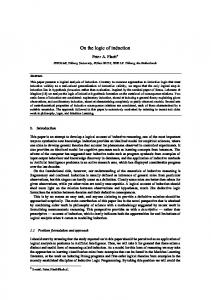
2 Input Data Specification The total data set [8], contains 260 data pairs (20x13) which are divided into two datasets. The basic data set will be used for forming the generalized profile function model and the validation dataset will be used for verification of the obtained generalized model. In our case we have used 13 data pairs for every object. In fact, in the considered case 14 objects will be used to get the generalized profile function model and verification will be performed using 6 new objects. The basic statistics of the measured data, that is, of the input data sets are presented in the Table 1. Scatterplot of the total dataset is presented in Fig.1 and the histogram of the validation dataset is shown in Fig.2.
_______ *Research is supported by the Ministry of Science, Republic of Serbia, as part of the project: EE 273015.B
ISSN:1790-5109
179
ISBN: 978-960-474-002-4
2nd EUROPEAN COMPUTING CONFERENCE (ECC’08) Malta, September 11-13, 2008
many different biological processes NN ensure smaller modeling error than the classical methods based on polynomials, exponential functions, or even on the specific functions. A typical structure of a NN is three-layer feed forward NN. The commonly used activation functions of neural networks include linear functions for output neurons, logistic sigmoid functions for hidden neurons, and identity functions for input neurons. It is known that the best model for the observed data is obtained if a minimal number of neural network layers and neurons is used [12, 13]. In other words it is necessary to use NN with low Vapnik-Chervonenkis (VC) dimension. VC dimension is determined simply by the number of free model parameters, that is by number of tansig neurons in the second (hidden) layer. The tansig neurons have logistic sigmoid tangent hyperbolic transfer function. The method of structural risk minimization (SRM) provides a systematic procedure for achieving the best performances by controlling the VC dimension [12, 13]. The controlling the VC dimension can be performed by decreasing, step by step, the number of tansig neurons in the hidden layers, [14]. In this study, a three layered feed forward NN with back propagation algorithm and with 2 tansing neurons in the hidden layer was used. As an example we shall consider two very different individual profile functions. The process of learning or training of NN for the first profile function is shown in Fig.3.
Table 1. Summary statistics of the input datasets Numb. Aver. of data
r [ c m] Total Dataset r Basic Dataset r Va l i d a t i o n Dataset r
Med.
SD
Min. Max.
260
8.1008 7.2000 5.9418 0.0 29.50
182
7.4975 6.3250 5.9019 0.0 29.50
78
9.5083 10.4250 5.8315 0.0 23.75
Scatterplot
0
10
20
30
r
Fig.1. Scatterplot of the total dataset
frequency
Histogram 1
10
30 25
0
10
20 Training errrors
15 10 5
-1
10
-2
10
0 -2
18
8
28
-3
10
r -4
Fig.2. Histogram of the measured values of the validation dataset
10
3 Individual Profile Functions Based on Neural Networks
10
20
30
40 Epoch
50
60
70
80
Fig.3. The process of learning for the first profile function
Artificial neural networks, in short, neural networks (NN), are very efficient and powerful tools of the computational artificial intelligence. In modeling ISSN:1790-5109
0
180
ISBN: 978-960-474-002-4
2nd EUROPEAN COMPUTING CONFERENCE (ECC’08) Malta, September 11-13, 2008
The second obtained individual profile function is presented in Fig.7.
Because of good convergence properties of the Levenberg-Marqurdt’s algorithm, this algorithm is used in the process of learning, [14]. In Fig.4, the first obtained (calculated) individual profile function is presented.
10
8
r [cm]
30
r [cm]
20
6
4
2 10 0 0
2
4
6
8
10
h [m]
Fig.7. The second individual profile function 0 0
10
20
Errors of modeling for the second profile function are shown in Fig.8.
30
h [m]
Fig.4. The first obtained individual profile function
0.4
Errors of fitting or modeling for the first profile function are shown in Fig.5 Error
0.2
0.4
0
0.2
-0.2
0
-0.4
Error
-
2
6
10
h [m]
Fig.8. Errors of modeling for the second profile function
-0.2
-0.4
10
20
h [m]
30
4 Generalized Profile Function Model In order to get the generalized model it is necessary, in the first step, calculates the normalized individual profile functions of all available objects. The normalization is performed by using the largest values on the x and y axis. In fact, the normalization of x axis is performed by H and of y axis by r(0). Two considered normalized profile functions are presented in Figs. 9 and 10.
Fig.5. Errors of modeling The process of learning for the second profile function is shown in Fig.6. 0
10
-1
10
0.8
-2
10
0.7 0.6 y
Training errrors
1 0.9
-3
10
0.5 0.4 0.3 0.2
-4
10
0
10
20
30
40 Epoch
50
60
70
80
0.1 0
Fig.6. The process of learning for the second profile function
ISSN:1790-5109
0
0.2
0.4
0.6
0.8
x
Fig. 9 The first normalized profile function
181
ISBN: 978-960-474-002-4
1
2nd EUROPEAN COMPUTING CONFERENCE (ECC’08) Malta, September 11-13, 2008
5 Basic Statistics of the Estimated Data
1
In the application of artificial intelligence (neural networks) and verification of the obtained results it is typical to use two datasets, the basic (model) and validation dataset. The validation dataset can contain the same amount of data as the basic dataset, but more frequently it is smaller. In our case the validation dataset is about 40% of the basic dataset. Testing the model accuracy with the validation dataset we shall get the real model accuracy. Evidently, it is better to use more validation datasets. If we validate the model with the same data used during model derivation, we shall get the initial model accuracy. Usually, the initial model accuracy is higher than the real. The summary statistics of the estimated data (data based on the GPFM) for the validation and basic dataset are given in Table 2.
0.9 0.8 0.7 0.6 y
0.5 0.4 0.3 0.2 0.1 0
0
0.2
0.4
0.6
0.8
1
x
Fig. 10 The second normalized profile function The generalized model, the GPFM, is obtained as a mean or average value of all available normalized individual profile functions. The obtained generalized model is presented in Fig.11.
Table 2. Summary statistics of the estimated data of both the validation and basic datasets
1 0.9
r [ c m] 0.8
Med.
SD
Min.
Max.
Basic Dataset 182 7.4744 6.3828 5.8483 0.0204 29.6145 Va l i d a t i o n 78 9.2297 10.0040 5.6736 0.0671 22.6973 Dataset
0.7 0.6 y
Num. Aver. of data
0.5
As we expected, a better agreement between the measured and estimated data, from the point of view of the average value, exists for the basic dataset, 7.4975 and 7.4744, than for the validation dataset, 9.5083 and 9.2297, Tables 1 and 2. Histogram of the estimated values of the validation dataset is shown in Fig. 12.
0.4 0.3 0.2 0.1 0
0
0.2
0.4
0.6
0.8
1
x
Histogram frequency
Fig.11. The generalized model Now, the generalized model presented in Fig.11 can be used for generating an approximation of any individual profile function. Renormalization is performed so that each individual (renormalized) profile function passes through the characteristic points (x0, y0 ), (x0 breast height, 1.3m, y0 = D /2 radius at breast height) and the final point (H,0). In accordance with this, the renormalization per x axis is performed using H, and per y axis using y(0) where:
30 25 20 15 10 5 0 -2
8
18
28
r
y(0) = [(D /2) / [y (1.3 /H)] Fig. 12. Histogram of the estimated values of the validation dataset
The value y(1.3 /H) is obtained using the generalized model, Fig. 11.
It can be seen, Figs. 2 and 12, that a good agreement between the histograms for the measured
Quality and performances of the obtained GPFM, will be analyzed in the subsequent sections. ISSN:1790-5109
182
ISBN: 978-960-474-002-4
2nd EUROPEAN COMPUTING CONFERENCE (ECC’08) Malta, September 11-13, 2008
and estimated values is achieved. The histograms of the measured and estimated values for the basic dataset are given in Appendix A, figs. A1 and A2. Also, based on these figures, we can conclude that a better agreement between the histograms is achieved for the basic dataset.
S = 0.60704 R = 0.99463 32 28
r [GPFM ] [cm]
24
6 Testing of the Obtained Generalized Model Usability of the obtained generalized model, in fact, the GPFM, will be tested by comparing the measured and estimated data using the regression analysis technique. Testing the accuracy of the generalized model is practically performed by computing the correlation coefficients between the measured and estimated data for both available dataset. The result of testing for the validation dataset is presented in Fig.13.
20 16 12 8 4 0 0
4
8
12
16
20
24
28
32
r (measured) [cm]
Fig. 14. Comparison measured and estimated data (the basic dataset)
S = 0.66236 R = 0.99325 32
The second pair of results gives the statistical performance of data comparison. This pair contains the regression parameters, the standard error of estimate, S and the correlation coefficient R. Values of the statistics of data comparison by the regression analysis are presented in Table 3.
28
r [GPFM ] [cm]
24 20 16
Table 3. Values of the statistics of data comparison by the regression analysis
12 8 4
S t a t i s t i c s o f t h e r c o mp a r is o n
0 0
4
8
12
16
20
24
28
Interc. a
32
r (measured) [cm]
Basic Dataset 0.0849 0.9856 Va l i d a t i o n Dataset 0.0412 0.9664
Fig. 13. Comparison measured and estimated data (the validation dataset)
Std.Err. S
Corr. coeff. R
R 2 [%]
0.6070
0.9946
98.93
0.6624
0.9933
98.65
As we expected, the parameter b, the slope of regression line, is closer to 1.0 in the case of the basic dataset, 0.9856, than in the case of the validation dataset, 0.9664. Also, the standard error is lower, 0.6070, compared to 0.6624 and the correlation coefficient is higher, 0.9946 than 0.9933. Unexpectedly, the intercept on y axis, a, is lower for the validation dataset, 0.0412 compared to 0.0849 for the basic dataset. Using the same dataset for modeling and validation, Korol and Gadow [6] have obtained a lower standard error, 0.526, compared to 0.607, but a worse correlation coefficient, 0.9820, compared to 0.9946 in the our case.
Computing the correlation coefficient between the measured and estimated data for the basic dataset is also done. The result of testing is presented in Fig.14. The first pair of results of the comparison represents the intercept on the y axis, a, and the slope of the regression line, b. Evidently, the regression line in the ideal case has to start from the origin and has to have the slope of 450. In other words the parameter a has to have value near 0 and the parameter b near 1.0.
ISSN:1790-5109
Slope b
183
ISBN: 978-960-474-002-4
2nd EUROPEAN COMPUTING CONFERENCE (ECC’08) Malta, September 11-13, 2008
[10] Roadknight, C. M., G.R. Balls, G. E. Mills, and D. Palmer-Brown, “Modeling complex environmental data“, IEEE Trans. Neural Net., vol.8, pp. 852-862, 1997. [11]] Georgina Stegmayer, Marko Pirola, Giancarlo Orengo and Omar Chiotti: “Towards a Volterra series representation from a Neural Network model“, Proceedings of the 5th WSEAS Int. Conf. on Neural Networks and Applications, Udine, Italy, March 25-27, 2004. [12] Haykin, S. Neural Networks: A Comprehensive Foundation, Macmillan College Publishing Company, New York, 1994. [13] Vapnik, Vladimir N., “An Overview of Statistical Learning Theory“, IEEE Transaction on Neural Networks, vol.10, no.5, Sept. 1999. [14] Beale, Mark, “Neural Network Toolbox“ NN Toolbox, Version 6.0.0.88, Release12, September 22, 2000, MATLAB 6 R12.
7 Conclusion It is shown that the generalized profile function model can be very successfully used in the process of estimating the individual profile functions. The obtained histograms for the measured and estimated data based on the GPFM are very similar. This conclusion is valid for both the validation and basic datasets. Also, the correlations coefficients between the measured and estimated data are very high, over 0,99 for both datasets. References: [1] Zhang,Q.-B.,Hebda, R.J.,Zhang, Q.-J. and Alfaro, R.I. “Modelling Tree-Ring Growth Responses to Climatic Variables Using Artificial Neural Networks“, Forest Science, vol. 46, no. 2, Society of American Foresters, Grosvenor Lane, Bethesda, pp. 229-239, 2000. [2] Hanewinkel, M.: “Neural networks for assessing the risk of windthrow on the forest division level: a case study in southwest Germany“, Eur. J. Forest Res. 124: 243-249, 2005. [3] Radonja, Pero, and Stankovic Srdjan, “Modeling of a highly nonlinear stochastic process by neural Networks“, In: Recent Advances in Computers, Computing and Communications Editors: N. Mastorakis and V. Mladenov, Published by WSEAS Press., 2002. [4] Radonja Pero, Srdjan Stankovic i Zoran Popovic: “Specific Process Models Obtained From General Ones“, WSEAS TRANSACTIONS on SYSTEMS, Issue 7, vol. 3, Pub. by WSEAS Press, Athens, pp. 2490-2495, 2004. [5] Hui, G.Y., von Gadow, K., “Entwicklung und Еrprobung eines Еinheitsschaftmodells fuеr die Baumart Cunninghamia lanceolata“. (in German) Forstw Cbl 116: 315-321, 1997. [6] Korol M.,von Gadow, K. “Ein Einheitsschaftmodell fuer die Baumart Fichte“ (in German) Forstw Cbl 122: 1-8, 2003. [7] Radonja, P., S. Stankovic, D. Drazic and B. Matovic.: “Generalized Models Based on Neural Networks and Multiple Linear Regression.“ In Proceedings of the 5th WSEAS Int. Conf. on CSECS 2006, Dattatreya, G. R. and James P. Durbano. (eds.). CDROM, Pub. by WSEAS Press, Dallas, USA, 2006, pp. 279-284. [8] Maunaga Z. “Productivity and structural characeristics of same-old stand of spruce in Republic Serbian“, (in Serbian). Ph.D. dissertation, Faculty of forestry, Belgrade, 1995. [9] Lek, S., A. Belaud, P. Baran, I. Dimopoulos and M. Delacoste, “Application of neural networks to modelling nonlinear relationships in ecology“, Ecol. Model., vol. 90, pp.39-52, 1996.
ISSN:1790-5109
Appendix A Histogram
frequency
80 60 40 20 0 -2
8
18 r
28
38
Fig. A1 Histogram of the measured values of the basic dataset frequency
Histogram 80 60 40 20 0 -2
8
18 r
28
38
Fig. A2 Histogram of the estimated values of the basic dataset
184
ISBN: 978-960-474-002-4