Artificial Immune Systems Applied to Multiprocessor Scheduling Grzegorz Wojtyla1 , Krzysztof Rzadca?,2,3 , and Franciszek Seredynski2,4,5 1
5
Institute of Computer Science, Warsaw University of Technology, Nowowiejska 15/19, 00-665 Warsaw, Poland 2 Polish-Japanese Institute of Information Technology, Koszykowa 86, 02-008 Warsaw, Poland 3
[email protected] Laboratoire Informatique et Distribution, 51 avenue Jean Kuntzmann, 38330 Montbonnot Saint Martin, France 4 Institute of Computer Science, University of Podlasie, Sienkiewicza 51, 08-110 Siedlce, Poland
[email protected] Institute of Computer Science, Polish Academy of Sciences, Ordona 21, 01-237 Warsaw, Poland
Abstract. We propose an efficient method of extracting knowledge when scheduling parallel programs onto processors using an artificial immune system (AIS). We consider programs defined by Directed Acyclic Graphs (DAGs). Our approach reorders the nodes of the program according to the optimal execution order on one processor. The system works in either learning or production mode. In the learning mode we use an immune system to optimize the allocation of the tasks to individual processors. Best allocations are stored in the knowledge base. In the production mode the optimization module is not invoked, only the stored allocations are used. This approach gives similar results to the optimization by a genetic algorithm (GA) but requires only a fraction of function evaluations.
1
Introduction
Parallel computers, ranging from networks of standard PCs to specialized clusters, supercomputers and the Grid, are becoming very popular and widely used. However, such systems are more difficult to use than the standard ones. Especially, mapping and scheduling individual tasks of a parallel program onto available resources is, excluding some very bounded conditions, NP-hard. Heuristic approaches to scheduling have been extensively studied [7] [6]. However, usually those algorithms are not very robust and work well only on certain types of programs. Search-based methods, which employ some global optimization meta-heuristics, were also used [10]. Nevertheless, those algorithms suffer from a large execution time which usually does not compensate the increased quality of the solutions [9]. Certainly a fast ?
Krzysztof Rzadca is partly supported by the French Government Grant number 20045874
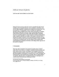
a)
b)
Fig. 1. An example system (a) and program (b) graphs. On the program graph, the top number shows the label of the task, the bottom one – the time necessary for computation. Vs = {P 0, P 1}; Es = {P 0 ↔ P 1}; Vp = {0, 1, 2, 3}; Ep = {0 → 1, 0 → 2, 2 → 3};
scheduler which could adapt to the conditions on a particular system would be more efficient. In this paper we propose a novel approach to scheduling parallel programs based on AIS. Our system performs population-based optimization in order to find an approximation of the optimal schedule. It also extracts the knowledge from individual schedules, stores it and uses it later to provide near-optimal schedules for similar parallel programs without running the optimization module. This paper is organized as follows. Section 2 gives a description of the scheduling problem considered. Section 3 outlines the concept of AIS. In Section 4 we present a scheduler which uses AIS. Experiments and results are described in the Section 5. We conclude the paper and present some directions of further works in Section 6.
2
Scheduling Parallel Programs
The architecture of the system on which the program is scheduled is described by a system graph, Gs = (Vs , Es ) (Figure 1a). The nodes Vs , called processors, represent processing units. The edges Es represent connections between processors. We assume homogeneous model – the time needed for computation of a task is the same on each processor. The parallel program to be scheduled is represented by a directed acyclic graph (DAG), Gp = (Vp , Ep ), where Vp = {vp } is a set of n ≡ |Vp | nodes representing individual, indivisible tasks of the program (Figure 1b). Later we will use the terms node and task interchangeably. The weight of a node vi gives the time needed for the computation of this task. Ep = {ei,j } is the set of edges which represent dependencies and communication between the nodes. If the nodes vi and vj are connected by an edge ei,j , the task vj cannot start until vi finishes and the data is transmitted. During the execution of the program a task vj is called a ready task, if all such vi are finished. The weight of an edge ei,j defines the time needed to send the data from the task vi to vj if those two tasks execute on neighboring processors. If those tasks execute on the
same processor we assume that the time needed for the communication is neglectable. If there is no direct link between the processors, the time needed for communication is a product of the edge’s weight and the minimum number of hops (distance) between processors. We assume that, once task’s execution has begun, it cannot be interrupted until the task finishes (i.e. non-preemptive model). We also assume that each task is executed on exactly one processor – we do not allow task duplication. Our system minimizes the total execution time (makespan) T of the program. We assume that T is a function of allocation and scheduling policy: T = f (alloc, policy). The scheduling policy determines the order of the execution of conflicting tasks on processors. Firstly, it ranks the tasks according to some criteria based on the program graph, such as the size of the sub-tree of the node (which will be used later in our experiments), the sum of computation costs on the longest path between the node and the sink node (s-level), or others [8]. If, during the program’s execution, two or more tasks assigned to the same processor are ready, the one with higher rank is chosen. We consider that the policy is given a priori. The allocation is a function which determines the processor on which each task of a program will be executed: alloc : Vp → Vs . Given the allocation and the policy it is trivial to schedule tasks onto processors.
3
Artificial Immune Systems
Biological immune systems can be viewed as a powerful distributed information processing systems, capable of learning and self-adaptation [2]. They have a number of interesting features [4], which include totally distributed architecture, adaptation to previously unseen antigens (molecules foreign to the system), imperfect detection (system detects antigens which match receptors even partially) and memory. They are a source of constant inspiration to various computing systems, called Artificial Immune Systems (AIS). Some of the previous attempts to use an AIS to solve computing problems include binary pattern recognition, scheduling [5], or intrusion detection in computer networks. AIS act upon a population of antibodies (responsible for antigen detection and elimination) which are modified in function of the affinity between antibodies and antigens [3]. In pattern recognition, the degree of affinity is proportional to the match between an antibody and an antigen, randomly chosen from a set of patterns to recognize. In optimization, where there is no explicit antigen population, antibody represents a point in the search space, so its affinity is related to the value of the objective function for this point. The antibodies which match the antigen best (which have highest affinity) are cloned. The number of clones produced is proportional to the affinity of the antibody. Then the clones undergo a process called hypermutation, with the probability of mutation inversely proportional to the parent’s affinity. The clones are then evaluated and some of the best ones replace their parents, if they have better affinity. The worst antibodies are replaced by new ones, either randomly initialized or created by immunological cross-over [1].
4
Immune-Based Scheduler
In real-world applications, similar programs are presented to the scheduler repeatedly. This can be caused by typical development cycle (run – debug – modify), or by running the same program on similar datasets. This suggests that one can store previous solutions to the scheduling problem and try to use it when scheduling new programs. Immune-based scheduler (IBS) is composed of the coding module, the knowledge base (KB) and the optimization module. The coding module encodes the DAG of every program entering the system by reordering individual tasks according to the schedule produced for a single processor by a list scheduling algorithm. The system then acts on encoded programs. KB stores the information about previous allocations, so it can be reused when allocating similar programs. The optimization module is responsible for searching the possible allocation space and delivering the approximation of the optimal allocation. Our system works in either learning or production mode. The learning mode can be viewed as a vaccination of the system by new antigens – programs to be allocated. The system learns how to deal with the antigen (how to allocate it) by producing antibodies (possible allocations) and evaluating them. The shorter the schedule produced by allocating the program with the antibody, the better the affinity of the antibody. The best antibody found is then saved in the KB. In the production mode the system does not have time to perform the optimization. Based on the knowledge stored in KB, it must quickly provide an immunological answer (an allocation) for a given program.
4.1
Learning Mode
When a new program (containing of n ≡ |Vp | tasks) is presented to the system running in the learning mode, after the initial encoding, the optimization module is invoked. We use an artificial immune system to find an approximation of the optimal allocation. One can, however, use any global search method, such as a GA, which returns an approximate optimal allocation of a given program. In our implementation, each individual represents a possible allocation of the program. The kth gene of the individual determines the allocation of the kth encoded task (a task vj which would be executed as kth on a single processor). Such an encoding does not produce any unfeasible individuals. The initial population of solutions is either totally random or formed partly by random individuals and partly by individuals taken from the knowledge base (adjusted to the length of the program by the algorithm described in the next section). Firstly, the algorithm computes the makespan Ti for each individual i by simulating the execution of the program with the allocation encoded in the individual i. Then the population is ranked – the best individual (the one with the shortest makespan) is assigned the rank r = 0. Then, a following optimization algorithm is run: repeat until endAlgorithm
1. clonal selection: the best I individuals are cloned. The number of clones Ci produced for the individual i is inversely proportional 0 , where C0 , the number of to the rank r of the individual: Ci = C 2r clones for the best individual, is a parameter of the operator. 2. hypermutation: each clone is mutated. The mutation ratio of the individual i is inversely proportional to the rank r of the clone’s parent. The number k of genes to mutate is given by k = round (P0 ∗ (1 + ∆P ∗ r) ∗ n) , where P0 is the average probability of gene’s mutation in the best individual, increased by ∆P for each following individual. The algorithm then randomly selects k genes and sets them to a random value. 3. clones’ evaluation: the makespan T is computed for each clone. 4. merging: K best clones are chosen. Each one of them replaces its parent in the population if the length of the clone’s schedule is less than parent’s. 5. worst individual replacement: L worst individuals from the population are replaced by randomly initialized ones. 6. immunological cross-over: M worst individuals of the population (excluding those modified in the previous step) are replaced by individuals created in the cross-over process. Each new individual has three parents, randomly chosen from the population and sorted by their ranks. If the best two parents have the same value of a gene, it is copied to the child. If they differ, the value for the gene is selected at random from the values of this gene in two best parents. However, the value equal to the value of this gene in the worst (third) parent has much smaller probability. We end the algorithm after a limited number of iterations or sooner if the best individual does not change for a certain number of iterations. The result of the algorithm is the best allocation found for a given program. The individual representing the best allocation is then stored in the KB.
4.2
Production Mode
In the production mode when a new program enters the system the optimization module is not invoked. Firstly, the program is encoded. Then a temporary population of allocations is created. The system copies to the temporary population each allocation from the KB adjusted to the length of the program. If the length k of the allocation taken from the KB is equal to the number n of tasks in the program, the unmodified allocation is copied to the temporary population. If k > n, the allocation in the temporary population is truncated – the first n genes are taken. If n < k, the system creates CloneNum ∗ ((n − k) + 1) allocations in the temporary population (CloneNum is a parameter of the algorithm). In each newly created allocation the old genes are shifted (so that every possible position is covered). Values for the remaining n − k genes are initialized randomly. In the next step the system finds the best allocation in the temporary population. The execution of the program is simulated with each allocation and the resulting makespan T is computed. The allocation which gives the minimum makespan T is returned as the result.
Table 1. Comparison of the IBS running in the learning mode, the EFT and the GA. program graph tree15 g18 gauss18 g40 g25-1 g25-5 g25-10 g50-1 g50-5 g50-10 g100-1 g100-5 g100-10
5
ETF 9 46 52 81 530 120 78 938 235 181 1526 460 207
Tbest GA 9 46 44 80 495 97 62 890 208 139 1481 404 176
IBS 9 46 44 80 495 97 62 890 210 139 1481 415 177
Tavg GA 9 46 44.3 80 495 97.8 70.2 890 213.3 146.4 1481 409.7 178.3
IBS 9 46 44 80 495 97 65.4 890 215.1 148.4 1481 421.1 180.9
evaluations [∗103 ] GA IBS 10.2 17.6 10.2 17.6 11.4 19.9 10.4 17.8 11.1 18.6 11.6 23.5 12.8 27.1 12.1 19.9 19.7 39.9 16.6 44.4 11.9 20.2 32.7 43.1 20.3 42.3
Experimental Results
We tested our approach by simulating the execution of programs defined by random graphs and graphs that represent some well-known numerical problems. The name of the random graph contains an approximate number of nodes and the communication to computation ratio (CCR). We focused on the two-processor system. We compared our approach (IBS) with a list-scheduling algorithm (EFT, homogeneous version of HEFT [9]) and a GA. The GA we used operates on the same search space as the IBS and is a specific elitist GA, with cross-over only between the members of the elite. We used sub-tree size as the scheduling policy in both the GA and the IBS. The parameters of the GA were tuned for the most difficult problem we considered (g100-1 ). The IBS parameters where then fixed so that both algorithms perform a similar number of function evaluations in one iteration. The parameters of the IBS are as follows: PopulationSize = 200, I = 60, C0 = 75, P0 = 0.10, ∆P = 0.05, K = 60, L = 70, M = 75. In the production mode, only one allocation was produced for each possible shift (CloneNum = 1). Both algorithms were ended if the best individual was the same during NoChangeIter = 50 iterations, but not later than after 1000 iterations. We run each algorithm on each program graph ten times. The shortest makespan found in ten runs Tbest and the average from the ten makespans Tavg are presented. We also present the average number of function evaluations in ten runs, as this value gives a good estimation of the run time of the algorithm. In the first set of experiments we compared the results of the GA and the IBS running in the learning mode (Table 1). As the values returned by both algorithms are very similar, we suppose that the search space is explored well by both approaches. On the easier graphs (tree15,g18 ) both algorithms found the optimal values in the first or the second iteration. However, in the harder graphs (e.g. g100-1 ) when we tried to
limit the number of function evaluations performed by the IBS algorithm (for example by reducing the NoChangeIter parameter), the values returned were deteriorating quickly. When comparing the results with the EFT algorithm, we observed that on harder graphs the difference in the length of schedules produced is about 5% to 30%. One can see that the higher the CCR, the longer makespan is produced by the EFT. The results of this experiments show that the global search method we use in the learning mode efficiently scans the search space and delivers results as good as a GA. They do not, however, show that our search algorithm performs better that the GA, because our algorithm performs twice as many function evaluations.
Table 2. Comparison of the IBS running in the production mode, the EFT and the GA. program graph tree15→g18 g40→g18 g40→g18→tree15 g25-1→g50-1 g25-1→gauss18 g40→g50-1 g25-1→g100-1 g50-1→g50-5
ETF 55 127 136 1468 582 1019 2056 1173
Tbest GA 55 126 135 1385 539 970 1976 1102
Tavg IBS 55 127 138 1424 550 978 2002 1146
GA 55 126 135 1385.2 541.7 970 1976.5 1106
IBS 55.7 129.4 139.4 1436 565.9 988 2025.4 1156.1
evaluations [∗103 ] GA IBS 10.4 0.1 11 0.3 11.5 0.4 18.7 0.6 14.8 0.2 15.1 0.7 19.7 1.1 35.4 0.9
In the second set of experiments we tested the immunological features of our system. Firstly we had run the IBS system in the learning mode on all the graphs. The best allocation found for each graph had been stored in the KB. Then we prepared some new graphs by joining all the exit nodes of one program graph with all the entry nodes of the other graph with edges with 0 communication costs. Table 2 summarizes the results obtained. We can see that our system is able to store knowledge and reuse it to schedule efficiently new programs. The results returned by the IBS running in the production mode are very close to those obtained by the GA. However, the IBS needs only a fraction of function evaluations needed by the GA. One can argue that the function evaluations “saved” in the production mode are used in the learning phase. We cannot agree with this. In the typical parallel systems schedulers are invoked repeatedly and with very tight time limits. Such a system really needs a fast scheduler in order not to waste too much processor time just to preprocess users’ programs. The other factor is that the overall load of the system is very uneven. On one hand, there are peaks, when many jobs are waiting in the queue (e.g. before a deadline of an important conference). On the other, periods (e.g. normal weekends) when most of the processors are unused. System administrator can use those free periods to run the learning phase of the IBS. Comparing the IBS and the EFT results, our system performs constantly better on harder graphs,
even when taking into account the average from the length of schedule returned. Nevertheless, the advantage the IBS had in learning mode (5% to 30%) is reduced to 2%–5%.
6
Conclusion and Future Work
This paper presents a new approach for scheduling programs given by a DAG graph. The most important result presented here is the ability to extract the knowledge from previous schedules and to use it when scheduling new, potentially similar, programs. After the initial phase of learning our system can provide a near-optimal schedule for previously unseen problems quickly. The results presented here open very promising possibilities for further research. We plan to construct new schedules from the knowledge base more carefuly. We also plan to deconstruct both the system and the program graph. Instead of storing schedules of complete programs on the whole system, we would like to schedule parts of graphs on locallydescribed parts of system.
References 1. H. Bersini. The immune and the chemical crossover. IEEE Trans. on Evol. Comp., 6(3):306–314, 2002. 2. D. Dasgupta. Information processing in the immune system. In D. Corne, M. Dorigo, and F. Glover, editors, New Ideas in Optimization, pages 161–165. McGraw-Hill, London, 1999. 3. L.N. de Castro and F.J. Von Zuber. Learning and optimization using the clonal selection principle. IEEE Trans. on Evol. Comp., 6(3):239–251, 2002. 4. P.K. Harmer, P.D. Williams, G.H. Gunsch, and G.B. Lamont. An artificial immune system architecture for computer security applications. IEEE Trans. on Evol. Comp., 6(3):252–280, 2002. 5. E. Hart and P. Ross. An immune system approach to scheduling in changing environments. In GECCO-99: Proceedings of the Genetic and Evol. Comp. Conference. Morgan Kaufmann. 6. E. Hart, P. Ross, and D. Corne. Evolutionary scheduling: A review. Genetic Programming and Evolvable Machines, 6(2):191–220, 2005. 7. Y.-K. Kwok and I. Ahmad. Static scheduling algorithms for allocating directed task graphs to multiprocessors. ACM Computing Surveys, 31(4):406–471, 1999. 8. F. Seredynski and A.Y. Zomaya. Sequential and parallel cellular automata-based scheduling algorithms. IEEE Trans. on Parallel and Distributed Systems, 13(10):1009–1023, 2002. 9. H. Topcuoglu, S. Hariri, and M.-Y. Wu. Performance-effective and low-complexity task scheduling for heterogeneous computing. IEEE Trans. on Parallel and Distributed Systems, 13(3):260–274, 2002. 10. A.S. Wu, H. Yu, S. Jin, K.-C. Lin, and G. Schiavone. An incremental genetic algorithm approach to multiprocessor scheduling. IEEE Trans. on Parallel and Distributed Systems, 15(9):824–834, 2004.