VOL. 7, NO. 4, APRIL 2012
ISSN 1819-6608
ARPN Journal of Engineering and Applied Sciences ©2006-2012 Asian Research Publishing Network (ARPN). All rights reserved.
www.arpnjournals.com
ARTIFICIAL NEURAL NETWORK PREDICTIVE MODELING OF UNCOATED CARBIDE TOOL WEAR WHEN TURNING NST 37.2 STEEL 1
T. B. Asafa1 and D. A. Fadare2
Department of Mechanical Engineering, King Fahd University of Petroleum and Minerals, Dhahran, Saudi Arabia 2 Department of Mechanical Engineering, University of Ibadan, Ibadan, Nigeria E-mail:
[email protected]
ABSTRACT We report the development of a predictive model based on artificial neural network (ANN) for the estimation of flank and nose wear of uncoated carbide inserts during orthogonal turning of NST (Nigerian steel) 37.2. Turning experiments were conducted at different cutting conditions on a M300 Harrison lathe using Sandvic Coromant uncoated carbide inserts with ISO designations SNMA 120406 using full factorial design. Cutting speed (v), feed rate (f), depth of cut (d), spindle power (W), and length of cut (l) were the input parameters to both the machining experiments as well as the ANN prediction model while the flank wear (VB) and nose wear (NC) were the output variables. Nine different structures of multi-layer perceptron neural networks with feed-forward and back-propagation learning algorithms were designed using the MATLAB Neural Network Toolbox. An optimal ANN architecture of 5-12-4-2 with the Levenberg-Marquardt training algorithm and a learning rate of 0.1 was obtained using Taguchi method of experimental design. The results of ANN prediction show that the model generalized well with root mean square errors (RMSE) of 3.6% and 4.7% for flank and nose wear, respectively. With the optimized ANN architecture, parametric study was conducted to relate the effect of each turning parameters on the tool wear. The ANN predictive model captures the dynamic behaviour of the tool wear and can be deployed effectively for online monitoring process. Keywords: model, ANN, carbide inserts, Taguchi method, tool wear, NST 37.2 steel, turning, cutting speed, machining.
1. INTRODUCTION NST 37.2 is a grade of Nigerian commercial steels produced by the Delta Steel Company (Asafa, 2007). The steel is commonly deployed for the production of machine components and sometimes as structural members in building construction and other architectural edifices. With its wide applications in machining industries and the requirements for various machining operations to produce the desired end results, it becomes important to establish an optimized model for the prediction of tool wear during turning of this steel. Accurate prediction of the tool wear conditions is an essential prerequisite for reliable on-line tool condition monitoring system (Mursec and Cus, 2003; Cus et al., 1997) and such a system can be deployed for effective tool wear monitoring in our local machine tools industries. Without doubt, modern machining system requires tool wear monitoring and prediction systems for higher quality production. In precision machining, the surface quality of the manufactured part can be related to tool wear which contributes to the increase in the industrial interest for inprocess tool wear monitoring systems. One of the available methods is by the application of ANN. Prediction of tool wear/tool life and tool condition monitoring has been extensively studied using ANN by many researchers (Sick, 2002). Sunil and Sandra (2000) considered neural network as a parallel processing architecture in which knowledge is represented in the form of weights between highly interconnected processing elements. More details of ANN can be found elsewhere (Ozel and Nadgir, 2002).
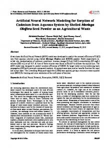
In the present study, ANN is adopted because of its several advantages. Among these is its capability to learn arbitrary nonlinear mappings between noisy sets of input and output data and predicting, with substantial accuracy, complex data interactions (Umbrello, et al., 2008. ANN differs from the traditional modeling approaches in that it is trained to learn solutions rather than being programmed to model a specific problem (Bhatikar and Mahajan, 2002). Also, it is usually used to address problems that are intractable or cumbersome to solve with traditional methods. A number of applications of ANN in tool conditioning monitoring and prediction of tool wear and tool life during non-orthogonal machining has been reported (Elanayar and Shin, 1990; Elanayar and Shin, 1992; Ghasempoor et al., 1999; Sick, 2002; Dimlar et al., 1997) or orthogonal turning (Li et al., 1999; Tansel, et al., 2000; and Dimlar, et al., 1998). ANN has equally been used for monitoring surface roughness (Asilturk and Cunkas, 2011) and induced residual stress (Umbrello, et al., 2008). In addition, ANN has found huge applications in other areas of industrial technology including semiconductor industries (Chen et al., 2007), transportation (Asafa et al., 2010) among others. ANN is often implemented via back propagation, a gradient descent algorithm in which the network weights are moved along the gradient of the performance function. The algorithm computes the weights in the network so as to minimize the output error in a least-squared sense (Howard and Mark, 2005). In the past, Boothroyd and Knight (1999) had observed that wear in metal cutting could be in the form crater (nose wear) or flank (as shown in Figure-1). Crater
396
VOL. 7, NO. 4, APRIL 2012
ISSN 1819-6608
ARPN Journal of Engineering and Applied Sciences ©2006-2012 Asian Research Publishing Network (ARPN). All rights reserved.
www.arpnjournals.com wear is the limiting factor for the tool life under very high speed cutting conditions because the wear is usually severe that the tool edge is weakened and consequently fractured. Crater wear occurs on the rake face of the tool, changing the tool-chip interface geometry, thus negatively affecting the cutting process. The most significant factors influencing the crater wear are the temperature at the toolchip interface and the chemical affinity between the tool and the work piece materials (Ezugwu et al., 2005). Flank wear occurs on the relief face of the cutting tool and is generally attributed to the rubbing of the tool along the machined surface. At high temperatures, abrasive and/or adhesive processes are accelerated, thus affecting tool material properties as well as work piece surface. Flank wear is a mechanically activated wear usually by the abrasive action of the cutting tools on the work piece material (Boothroyd and Knight, 1999). The severity of abrasion increases in cases where the work piece materials contain hard inclusions, or when there is hard wear debris from the work piece or the tool, at the interface (Ozel and Karpat (2005). Flank wear increases with increase in cutting time as well as increases in the axial cutting distance (Ozel and Nadgir, 2002). The nature of this relationship depends on material and process condition.
widely applied, it is however difficult to implement for online sensing because of the inaccessibility of the tool surface during machining (Xu, 2009). Indirect method of tool wear estimation has been extensively studied as a solution to the shortcomings of the direct method most especially for in-process monitoring. Matins et al. (1984) used vibration generated during cutting process to reveal the state of the tool wear. The change in the flank wear has also been monitored by means of reduction in the work piece dimensions (ElGomayel and Breggar, 1986). The use of acoustic emission due to change in sound intensity as well as optical method that relies on the changes in the reflectance characteristics of the worn tool surfaces has also been reported (Kannately-Asibu and Dornfeld, 1992). Also, spindle motor current and power have been used to estimate tool wear for on-line monitoring (Martins et al., 1984). Literature shows that tool wear prediction during machining of a wide range of steel grades have been reported (Ezugwu et al., 2005). However, it appears that no study has been conducted in the area of machining of NST 37.2. Therefore, developing an optimized ANNbased predictive model for estimation of flank and nose wear of uncoated carbide cutting tools during turning of NST 37.2 is the objective of this study. It is our opinion that these findings will assist machinists in acquiring a priori knowledge of the magnitude of tool wear without the usual experimental trials and errors approach. 2. MATERIALS AND METHODS NST 37.2 samples were used as the work piece material for the orthogonal turning experiment in a full factorial design. The outputs of the experiment were used to construct the predictive model while the architecture of the model was optimized via Taguchi approach using signal-to-noise ratio and analysis of variance. Details of these steps are discussed in this section.
Figure-1. Major regions of tool wear during metal cutting (Boothroyd and Knight, 1999). Tool wear are measured directly or indirectly (Cuneyt, 2009; Xu et al., 2011). Direct measurement is usually carried out by means of optical, radiometric, pneumatic or contact sensors in which tool wear is measured in term of material loss (Sunil Elanayar and Sandra, 2000). This technique can be effectively deployed for on-line measurement. The application of the tool maker microscopes and the radiometric method help us to measure the tool wear directly (Ozel and Nadgir, 2002). For example, Ezugwu et al. (2005) measured tool wear on ceramic inserts during machining of Inconel 718 by means of a travelling microscope. Though direct method is
2.1 Work piece material, cutting tool and tool holder Samples of fully annealed NST 37.2 steel bars with 25 mm diameter were obtained from Delta Steel Company (DSC). The chemical composition and the mechanical properties of the steel sample are given in Tables 1 and 2, respectively. Uncoated cemented carbide inserts produced by Sandvic Coromant® with ISO designation SNMA120406 were used as the cutting tool. The insert had a square shape with zero clearance angle and inbuilt chip breakers. It was rigidly mounted on a tool holder with ISO designation PSBNR 3225P15 while the holder was clamped to the tool post in an orthogonal arrangement.
Table-1. Chemical composition of NST 37.2 (Asafa, 2007). Element Composition (%W)
C
S
Si
Mn
P
Fe
0.33
0.01
0.150
0.69
0.02
98.80
397
VOL. 7, NO. 4, APRIL 2012
ISSN 1819-6608
ARPN Journal of Engineering and Applied Sciences ©2006-2012 Asian Research Publishing Network (ARPN). All rights reserved.
www.arpnjournals.com Table-2. Mechanical properties of NST 37.2 (Asafa, 2007). Properties
Average value
Yield strength (MPa)
245
Tensile strength (MPa)
342
Elongation (%)
18
Reduction in area (%)
15
Young modulus (GPa)
199
Brinell Hardness
49
Density (g/m3)
8.15
2.2 Machining experiment Straight turning was done on M300 Harrison-type lathe driven by 3.0 Hp Kapak inductions motor with speed range of 40-2500 rpm. Cutting conditions typical of those available in the machining industries were used for the machining trials. These cutting conditions are listed in Table-3. The cutting parameters - cutting speed (v); feed rate (f) and depth of cut (d) - were investigated at three different levels in a 33 full factorial experiment. Full factorial design is chosen to study the interactions between the turning parameters. Table-3. Summary of turning conditions.
Level 1
Cutting parameters Cutting speed Feed rate Depth of (m/min) (mm/rev) cut (mm) 20.4 1.0 0.2
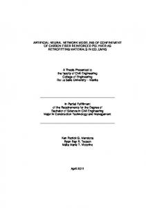
2.3.1 Data collection and processing Input data into the neural networks were obtained from the machining parameters used in the full factorial experiments. 112 input/output data were used for the network training, model validation and testing in a relative proportion of 2:1:1. The input vectors were first normalized with Matlab function, prestd, in order to obtain inputs with zero mean and unity variance. In addition, principal component analysis was done with Matlab function, prepca, to eliminate those components that contribute less than 99% to the variation in the datasets. The outputs of the network were later converted to the original data format with Matlab function postd. 2.3.2 Neural network design and optimization The design of the network architecture requires the selection of a number of hidden layers and those of the neurons in each of the hidden layer, the training algorithm and the learning rate that would minimize the prediction error. Figure-2 shows a general architecture of the ANN model having five inputs and two outputs as used in this work. Taguchi method is used to optimize the number of neurons in each of the hidden layers, the training algorithm and the learning rate based on the method proposed by Khaw et al. (1995). Three training algorithms which are Levenberg-Marquardt algorithm, Scaled Conjugate Gradient and Bayesian Regularization were included in the optimization because of their similar performance in some previous studies (Bealle at al., 2010). Two hidden layers were proposed since ANN model of one layer is usually too weak to accurately predict nonlinear function (Kaw et al., 1995).
2
29.1
1.8
0.4
Cutting speed (v)
3
42.4
2.2
0.8
Feed rate (f) Flank wear
For each of the machining conditions, eight passes of 50 mm length of cut were made. At the end of each pass, the spindle motor current, nose wear and flank wear were measured. Spindle current was measured with digital multimeter connected to the electric motor of the lathe while the nose and flank wear were measured by means of a machine vision system earlier developed at the University of Ibadan, Nigeria (Oni, 2007). The tool rejection criteria for roughing operation according to ISO 3685 Standard were used. The criteria directed that an insert must be rejected and further machining discontinued when any or combination of the following criteria is reached: flank wear ≥ 0.7 mm, nose wear ≥ 0.5 mm, or catastrophic failure. These values serve as constrains into the predictive model. 2.3 Neural network model description Here, we discuss the processes involved in the data collection, pre-processing and partitioning of data as the preliminary stages in ANN development. Then, the steps in the architecture design, training as well as testing of the neural network performance are explained.
Depth of cut (d) Nose wear
Length of cut (l) Spindle power (P) Input layer
Hidden layer
Output layer
Figure-2. Schematic illustration of the ANN structure. The four important parameters of ANN model are arranged using the Taguchi’s orthogonal array (Taguchi, 1993). These parameters are: (A) number of neurons in hidden layer 1, (B) number of neurons in hidden layer 2, (C) type of training algorithm and (D) learning rate. The number of neurons in each of the hidden layers is selected based on the mathematical relationship presented by Chen et al. (2007) (Table-4). Taguchi approach is essentially a statistical technique used in experimental study for analyzing the relationship between large numbers of design parameters with the smallest number of experimental runs (Chen et al., 2007). Taguchi used an engineering approach to plan
398
VOL. 7, NO. 4, APRIL 2012
ISSN 1819-6608
ARPN Journal of Engineering and Applied Sciences ©2006-2012 Asian Research Publishing Network (ARPN). All rights reserved.
www.arpnjournals.com OA and analyze the results using signal-to-noise ratio (S/N) approach to determine the optimal combination of parameters and using analysis of variance (ANOVA) to rank the parameters in order of influence/significance and (4) conducting a confirmatory experiment using the optimal ANN architecture (Hinkelmann and Kempthorne, 2005). The viability of this approach has been demonstrated for selection of ANN parameters for designing high quality and robust networks (Asilturk and Cunkas, 2011; Chen et al., 2007). In this work, the number of input variables (N) is 5 and that of the output variable (OP) is 2, each with three levels. The results are presented in Table-5.
and design optimum experimental runs using orthogonal arrays and signal-to-noise ratios. His method is widely applicable because of its strengths; it has however been criticized for the poor interaction among the processing variables. A reviewed article on the strengths and limitations of Taguchi’s experimental design approach had been published (Maghsoodloo et al., 2004). Generally, implementation of Taguchi method requires four basic steps. These include (1) brainstorming on the design parameters that are important to the process and identify the factors as well as the levels of each factor, (2) selecting the appropriate orthogonal array (OA) from the published table, (3) conducting experiments based on the selected
Table-4. Estimation of number of neurons in the hidden layers. ANN parameter Number of neurons in the Number of neurons in the hidden hidden layer 1 layer 2
Level
N + OP 2
Level 1
N + OP
Level 2
2N +1
Level 3
OP x ( N + 1)
2N + 1 3 OP x ( N + 1 ) OP x ( N + 1 ) + 3 2N + 1+
Table-5. Factor and level for the ANN parameters.
1
Number of neurons in the hidden layer 1 (A) 3
Factor Number of neurons in the hidden layer 2 (B) 4
Training algorithm (C) LM
Learning rate (D) 0
2
11
15
RP
0.05
3
12
16
SCG
0.1
Level
Table-6. L9 (34) orthogonal arrays and S/N ratio. Test run
Orthogonal array
S/N ratio
1
A1
B1
C1
D1
-25.766
2
A1
B2
C2
D3
-31.496
3
A1
B3
C3
D2
-57.066
4
A2
B1
C2
D2
-23.837
5
A2
B2
C3
D1
-29.758
6
A2
B3
C1
D3
-21.393
7
A3
B1
C3
D3
-22.726
8
A3
B2
C1
D2
-24.123
9
A3
B3
C2
D1
-23.897
399
VOL. 7, NO. 4, APRIL 2012
ISSN 1819-6608
ARPN Journal of Engineering and Applied Sciences ©2006-2012 Asian Research Publishing Network (ARPN). All rights reserved.
www.arpnjournals.com Table-7. S/N ratio and ANOVA. Level (dB)
Range
Rank
DOF1
SS2
Variance
% contr3
-23.58
14.52
1
2
384.98
192.49
39.34
-28.46
-34.12
10.01
4
2
151.14
75.57
15.44
-23.761
-26.41
-36.52
12.76
2
2
271.87
135.96
27.78
-26.473
-35.01
-25.22
9.80
3
2
170.58
85.29
17.43
8
7601.54
1
2
3
A
-38.109
-24.99
B
-24.109
C D Total
100
Figure-3. Response chart for the S/N ratio. Table-8. The optimized ANN model. Network architecture
Training algorithm
Learning rate
5-12-4-2
LM
0.1
Table-6 shows the arrangement of 4-factor, 3level design proposed to determine the effect of ANN variables on the network performance. For this type of an arrangement, 34 (or 81) sets of experimental runs are needed for full factorial design while only 9 suffice based on Taguchi method. For every experimental run, the training section is terminated if one of the following stopping criteria is reached: (a) when the mean square error (MSE) between the actual and predicted output
MSE (flank wear) 0.0365
MSE (nose wear) 0.0467
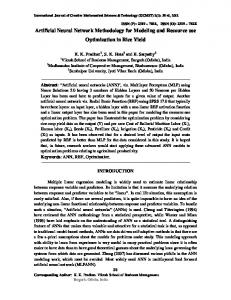
reaches 10-10, (b) when the number of iterations reaches 2000 and (c) when validation data begin to over fit. A typical example of the convergence of the testing and training networks for flank wear is shown in Figure-4. The best validation performance of 0.041 is obtained after 27 iterations. The coefficients of regression are 0.98 and 0.99 for training and testing data, respectively. These coefficients are statistically satisfactory.
400
VOL. 7, NO. 4, APRIL 2012
ISSN 1819-6608
ARPN Journal of Engineering and Applied Sciences ©2006-2012 Asian Research Publishing Network (ARPN). All rights reserved.
www.arpnjournals.com
(a)
(b) Figure-4. Network performance (a) Network validation with number of epochs (b) Regression analysis for training and validation datasets for flank wear. The MSE of the nine ANN architectures are taken as the outputs of the experimental runs and as the inputs to the S/N ratios. Depending on the optimization requirements, different S/N ratios may be applicable, including “lower is better” (LB) - minimum performance characteristics, “nominal is best” (NB) - medium performance characteristics, and “higher is better” (HB) maximum performance characteristics. Since the value of MSE is desired to be as small as possible for both flank and nose wear, LB is selected. The S/N ratio is therefore calculated from the Eq. (1) (Chen et al., 2007). The results are presented in Table-6.
⎛ N i y 2j ⎞ ⎟ ( S / N ) i = − 10 log ⎜ ∑ ⎜ u =1 N ⎟ i ⎠ ⎝
(1)
Where i = experimental number, j = number of trials, Ni = number of trial for experiment i and y is the trial output. After estimating the S/N ratio for each of the experimental runs (Table-6), the average S/N value is calculated for each factor and the corresponding level.
This is done by taking the average value of the S/N ratios for each level and the corresponding factor level. The results are presented as a response table (Table-7) and a response graph (Figure-3). The optimum parameter combination is A3B1C1D3 as highlighted in Table-7. Under this condition, the BPNN architecture is 5-12-4-2 with a Levenberg-Marquardt training algorithm and a learning rate of 0.1 as presented in Table-8. The relative contribution of each ANN parameter on the performance characteristic of the predictive model expressed as a percentage is obtained via ANOVA (Hsu et al., 2008). The results, shown in Table-7, indicate that the first hidden layer is the most significant parameter contributing ~39% to the change in the network performance while the second hidden layer is the least with ~15%. The learning rate and the training algorithm contribute ~17% and ~27%, respectively. 3. RESULTS AND DISCUSSIONS Once the optimal level of the design parameters has been selected with Taguchi method, we thereafter run
401
VOL. 7, NO. 4, APRIL 2012
ISSN 1819-6608
ARPN Journal of Engineering and Applied Sciences ©2006-2012 Asian Research Publishing Network (ARPN). All rights reserved.
www.arpnjournals.com
using the optimal level of the design
parameters 2003).
is
calculated
y predicted = y m + Where
ym
from
k
∑ (y i =1
i
(Lin
and
− ym )
is the global mean S/N ratio,
Chang,
(2)
yi
is the mean
0.8
0.08
0.9
1
0.7
0.07
0.8
0.9
0.6
0.06
0.7
0.8
0.5
0.05
(a)
0.4
0.04
0.3
0.03 Experimental flank w ear Predicted Flank w ear Experimental Nose w ear Predicted Nose Wear
0.2 0.1 0 0
200
0.02
Nose wear (mm)
Flank Wear (mm)
S/N ratios at the optimal level, and k is the number of the design parameters. Equation (2) gives -~20dB which is greater than -~21dB, the maximum value obtained from the orthogonal array. Experiment conducted at the optimum design parameters gives S/N ratio of -~20dB which is the same as the predicted value and higher than 21dB. The average prediction errors were 3.7% and 4.7% for flank and nose wear respectively. This gives a good confidence that the optimal parameters are truly optimal. With this level of accuracy, the model performance is satisfactory. The higher MSE of the nose wear is attributed to the fact that the two outputs were being predicted simultaneously and in such a case the output of the ANN model is often more accurate for the first output than the
0.01
400
0.7
0.6
0.6
0.5
(b)
0.4
Experimental flank w ear Predicted flank w ear Experimental nose w ear Predicted nose w ear
0.2
0 0
Cutting length (mm)
0.5 0.4
0.3
0.1
0 600
100
200 300 Cutting length (m m )
400
0.3 0.2 0.1 0 500
0.7
2 Experimental flank w ear Predicted Flank w ear Experimental Nose w ear Predicted Nose w ear
1.6 1.4
0.6 0.5
1.2
0.4
1 0.3
0.8 0.6
(c)
0.4 0.2 0 0
100
200 300 Cutting length ( mm)
400
Nose wear (mm)
1.8
Flank Wear (mm)
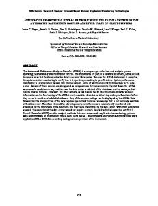
3.1 Model validation Three typical cutting conditions were selected to test the accuracy of the model. The results of these tests indicate that ANN is a viable tool for prediction of tool behaviour. Figure-5(a) shows that the flank and nose wear increased as the cutting length increased. This behaviour is well captured by the ANN model. It is however obvious that increase in flank wear is greater than that of the nose wear. This observation can be attributed to the tool nose radius (0.6 mm) being less than the depth of cut (0.8 mm). The analogy can be correlated to the direct proportionality between flank wear and the depth of cut as presented by Yongjin and Fischer (2002). However, the nose wear exceeded that of flank wear at the condition cutting condition when v = 20.42 mm/s, f = 2.2 mm/rev and d = 0.4 mm as showing in Figure-5(b). This behaviour is attributed to the depth of cut (0.4 mm) being smaller than the nose radius which subsequently lead to the partial engagement of tool nose during the turning operation. At higher cutting speed (42.42 mm/s), the flank wear becomes higher than the nose wear Figure-5(c) due to high temperature generated at high cutting speed. Such a high temperature could easily weaken the tool materials and thereby enhances tool wear.
Flank Wear ( mm)
y predicted
rest. We thereafter used the optimal ANN architecture to predict the outcome of the testing data. The result of the model is now compared with the experimental value.
Nose Wear (mm)
a confirmatory test to verify the improvement of the performance characteristic using the optimal level of the design parameters for the flank wear. The optimal combination of the factors level is the test with highest value of S/N ratio. The estimated optimum output
0.2 0.1 0 500
Figure-5. Comparison of ANN prediction and measured tool wear for various cutting conditions (a) v = 20.42 mm/s, f = 1.0 mm/rev, d = 0.8 mm (b) v = 20.42 mm/s, f = 2.2 mm/rev, d = 0.4 mm and (c) v = 42.42 mm/s, f = 2.2 mm/rev, d = 0.8 mm The feature that is common to both the experiment and the ANN predictive model is the ability to capture the cutting conditions where the resulting tool
wear violates the standard conditions for tool disposal. Few machining experiments were conducted such that the resulting tool wear were higher than the accepted values.
402
VOL. 7, NO. 4, APRIL 2012
ISSN 1819-6608
ARPN Journal of Engineering and Applied Sciences ©2006-2012 Asian Research Publishing Network (ARPN). All rights reserved.
www.arpnjournals.com In the same manner, the predictive model equally predicts the cutting conditions at which tool wear constrains are violated. This will surely guide machinist on the selection of the appropriate turning parameters without violating the wear constraints. 3.2 Effects of cutting parameters on tool wear Cutting speed is one of the most important parameters that influence the development of tool wear during machining. Figure-6 (a) and (b) show the progressive increase in both the flank and nose wear with increase in cutting speed within the experimental consideration. Both wear types are linearly related to the cutting speed with the correlation coefficients of 0.99 for both wear. The increase in tool wear at higher cutting speed can be explained by the enhancement of tool material diffusion and thermal stress inducement at higher
temperature. The tool wear are still within the acceptable level for the cutting conditions shown in Figure-6. Generally, when one of the cutting parameters is increased, wear mechanism due to diffusion and adhesion is activated. A similar correlation between feed rate and dept-of-cut, and process parameters such as cutting force, flank and nose wear has been reported (Ezugwu et al., 2005). The results of the ANN prediction for the influence of feed rate on tool wear are shown in Figure-7 (a) and (b). Increase in feed rate raises the thermal state of the tool with subsequent softening and eventual rise in the wear rate. The condition for continuous tool application is only satisfied at feed rate of 1 mm/rev for both wear. Higher wear is recorded for a feed rate greater than 1 mm/rev. This behaviour is also confirmed by Sivasakthivel et al. (2010).
(a)
(b)
Figure-6. Effects of cutting speed on tool wear (a) flank wear and (b) nose wear. 0.9
1.1 Flank w ear,V=29.06mm/s,DOC=0.2mm, L=300mm
0.8 N o se w ear (m m )
Flank Wear (mm)
1
(a)
0.9
0.8
0.7
(b)
Nose w ear, V=29.06mm/s,DOC=0.2mm, L=300mm
0.6 0.5 0.4
0.7
0.3
0.6 0.5
1
1.5
2
2.5
Feed (mm/rev)
0.5
1
1.5
2
2.5
Feed (mm/rev)
Figure-7. Neural network prediction on the influence of feed on tool wear: (a) flank wear (b) nose wear. The effect of depth of cut (DOC) on tool wear is shown in Figure-8 (a and b). The behaviour of tool wear under DOC modulation is in two folds. Between 0.2 mm and 0.4 mm, both the flank and nose wear decreased and thereafter increased between 0.4 mm and 0.8 mm. Thus the wear has minimum values at a depth of cut of 0.4 mm.
More study is required to identify the reasons for this behaviour. A typical tool wear image generated at cutting speed of 42.4 m/min is shown in Figure-2. Presence of chipping, attrition and abrasion were observed on the carbide tools during machining under the conditions investigated in this study.
403
VOL. 7, NO. 4, APRIL 2012
ISSN 1819-6608
ARPN Journal of Engineering and Applied Sciences ©2006-2012 Asian Research Publishing Network (ARPN). All rights reserved.
www.arpnjournals.com 1 0.5
0.95 0.9
Flank Wear, V=42.42mm/s,f=1.8mm/rev, L=200mm
0.85
0.4
0.8
Nose Wear (mm)
Flank wear ( mm)
Nose Wear,V=42.41mm/s,f=1.8mm/rev, L=200mm
0.45
0.75 0.7
(a)
0.65
0.35 0.3
0.6
0.2
0.55
0.15
0.5
(b)
0.25
0.1
0
0.2
0.4
0.6
0.8
1
0.1
0.3
Depth Of Cut (m m )
0.5
0.7
0.9
Depth Of Cut (m m)
Figure-8. Effect of depth of cut on tool wear: (a) flank wear (b) nose wear. condition of v = 42.42 mm/s, f = 1.8 mm/rev and l = 200 mm. However, minimum wear were obtained for flank and nose wear at d = 0.8 mm and 0.2 mm respectively for condition v = 29.06 mm/s, f = 2.2 mm/rev and l = 400 mm. The ANN predictive model captures the dynamic behaviour of the tool wear and can be effectively deployed for online monitoring process. REFERENCES Asilturk I. and Cunkas M. 2011. Modeling and prediction of surface roughness in turning operations using artificial neural network and multiple regression method. Expert Systems with Applications. 38: 5826-5832. Figure-9. A typical flank wear image generated at cutting speed of 42.4 m/min, feed rate f 1.8 mm/rev and depth-ofcut of 0.8 mm as observed on a tool insert (Fadare and Asafa, 2009). CONCLUSIONS We have used ANN to create a predictive model for the estimation of flank and nose wear during machining NST 37.2. The optimized architecture, obtained with Taguchi experimental design, was 5-12-4-2 with the Levenberg-Marquardt training algorithm and a learning rate of 0.1. The results of ANN prediction show that the model generalized well with root mean square errors (RMSE) of 3.55% and 4.67% for flank wear and nose wear, respectively. With the optimized ANN architecture, parametric study was conducted to show the effects of the cutting parameters on the tool wear. Generally, the magnitude of flank wear was significantly higher than that of the nose wear in all the cutting conditions considered except at cutting condition (v = 20.42 mm/s, d = 2.2 mm and f = 0.4 mm/rev) where the magnitude of the nose wear was higher than that of the flank wear. From the parametric study, increase in cutting speed accelerates tool wear. Increase in the feed rate increased both flank and nose wear. Depth of cut significantly affects the tool wear. A DOC of 0.4 mm produces least wear for cutting
Asafa T.B. 2007. Investigation on tool wear prediction and optimization of cutting conditions in Machining Aladja NST 37.2. Unpublished M.Sc. Dissertation of Mechanical Engineering Department, University of Ibadan, Nigeria. Asafa T. B., Ajayeoba A. O. and Adekoya L. O. 2010. Prediction of some anthropometric data of Bus Passengers using Artificial Neural Network: A case study of Molue bus in Lagos State, Nigeria. International Journal of Biological and Physical Sciences. 15(3): 345-356. Beale M. H., Hagan M. T. and Dewuth H. B. 2010. Neural Network Tool: Users' Guide in MATLAB Documentation, by MATLAB. Mathworks Corporation. pp. 160-170. Bhatikar S. R. and Mahajan R. L. 2002. Artificial neuralnetwork-based diagnosis of CVD barrel reactor. IEEE Transactions on Semiconductor Manufacturing. 15(1): 7178. Boothroyd G. and Knight W.A. 1989. Fundamentals of machine and machine tools. 2nd Ed. Marcel Dekker Inc. New York, USA. p. 230. Caldas L. G. and Norford L. K. 2002. A design of optimization tool based on a genetic algorithm. Automatic Constrain. 11(2): 173-184.
404
VOL. 7, NO. 4, APRIL 2012
ISSN 1819-6608
ARPN Journal of Engineering and Applied Sciences ©2006-2012 Asian Research Publishing Network (ARPN). All rights reserved.
www.arpnjournals.com Cook D. F., Ragsdale C. T. and Major R. L. 2000. Combining a neural network with a genetic algorithm for process parameter optimization. Eng. Appl. Artif. Intell. 13: 391-396. Cuneyt A. 2009. Tool wear condition monitoring using a sensor fusion model based on fuzzy inference system. Mechanical Systems and Signal Processing. 23(2): 539546. Cus F., Sokovic J., Kopac J. and Balic J. 1997. Model of complex optimization of cutting conditions. International Journal of material processing Technology. 64: 41-52. Daren Z. 2001. QSPR studies of PCBs by the combination of genetic algorithms and PLS analysis. Comput. Chem. 25: 197-204. Dimla D. E., Lister P. M. and Leighton N. J. 1997. Neural network solution to the tool condition monitoring problems in metal cutting - a critical review of methods. International Journal of Machine Tool and Manufacture. 37: 1219-1241.
Goldgerg D.E. 1999. Genetic algorithm in search of optimization and machine learning. Addison Wesley, USA. pp. 2-5. Howard D. and Mark B. 2005. Neural network tool box: MATLAB, Language of Technical Computing. p. 120. Hsu C.Y., Ko T.F. and Huang Y.M. 2008. Influence of ZnO buffer layer on AZO film properties by radio frequency magnetron sputtering. Journal of the European Ceramic Society. 28: 3065-3070. International Standard Organization (ISO). 1977. Tool life testing with single-point turning tool. International Organization for Standardization. Ref No: ISO 3685-1977. Islier A. A. 1998. A genetic algorithm approach for multiple criteria facility layout design. Int. J. Prod. Res. 36(6): 1549-1569. Kannately-Asibu J.E. and Dornfeld D.A. 1992. A study of tool using statistical analysis of metal cutting acoustic emission. Wear. 76: 247-261.
Elanayar S.V.T. and Shin Y.C. 1990. Machining condition monitoring for automation using neural networks. ASME Winter Annual Meeting, Dallas, TX, USA. pp. 85-100.
Khaw J. F. C., Lim B. S. and Lim L. E. N. 1995. Optimal design of neural network using the Taguchi method. Neurocomputing. 7: 225-245.
Elanayar S.V.T. and Shin Y.C. 1992. Robust tool wear estimation via radial basis function neural networks. ASME Winter Annual Meeting, Anaheim, C. A, USA. pp. 37-51.
Lin Z. C. and Chang D. Y. 2003. Tool wear investigation on the precision progressive die for the IC dam-bar cutting process. Int. Journal of Advanced Manufacturing Technology. 22: 344-356.
El-Gomayel J. I. and Breggar K. D. 1986. On-line tool wear sensing for turning operations. Tans. ASME, J. Eng. Ind. 108: 44-47.
Li X.P., Iynkaran K. and Nee A.Y.C. 1998. A hybrid machining simulator based on predictive machining theory and neural network modeling. Proceedings of CIRP International Workshop on Modeling and Machining Operations. Atlanta, Georgia, U.S.A. pp. 417-428.
Ezugwu E. O., Bonney J., Fadare D. A. and Wales W. F. 2005. Machining of Nickel-based Inconel 718, alloy with ceramic tool under finishing conditions with various coolants Supply pressures. Journal of International Processing Technology. 162-163: 609-614. Ezugwu E.O., Fadare D.A., Bonney J., Silva R.B. and Wales W.F. 2005. Modelling the correlation between cutting and process parameters in high-speed machining of Inconel 718 alloy using an artificial neural network. International Journal of Machine Tools and Manufacture. 45: 1375-1385. Fadare D.A and Asafa T. B. 2009. Performance evaluation of uncoated carbide. Proceedings of 22nd AGM and International conference of the Nigerian Institute of Mechanical Engineers, Osun. pp. 20-24. Ghasempoor A., Jeswiet J. and Moore T.N. 1999. Real time implementation of on-line tool condition monitoring in turning. International Journal of Machine Tool and Manufacture. 39: 1883-1902.
Martins K.F., Brandon J.A., Grrosvenor R.I. and Owen A. 1984. A comparison of in-process tool wear measurement methods in turning. Proc. 26th inter. MTDR Conf. p. 121. Mursec B. and Cus F. 2003. Integral model of selection of optimal cutting conditions from different databases of tool makers. International Journal of material processing Technology. 133: 158-165. Oni A. O. 2007. Development of a vision system with respect to tool wear and surface roughness measurement. Unpublished M.Sc. Dissertation. Mechanical Engineering Department, University of Ibadan, Nigeria. Ozel T. and Nadgir A. 2002. Prediction of flank wear by using back propagation neural network modeling when cutting hardened H-13 steel with chamfered and honed CBN tool. International Journal of Machine Tool and Manufacture. 42: 287-297.
405
VOL. 7, NO. 4, APRIL 2012
ISSN 1819-6608
ARPN Journal of Engineering and Applied Sciences ©2006-2012 Asian Research Publishing Network (ARPN). All rights reserved.
www.arpnjournals.com Richards E., Bessant C. and Saini S. 2002. Optimization of a neural network model for calibration of valtammetric data. Chemometrics and Intelligent Laboratory Systems. 61: 35-49. Sick B. 2002. On-line and indirect tool wear monitoring in turning with artificial neural network: a review of more than a decade of research. Mechanical System Signal Processing. 16: 487-546. Sivasakthivel P. S., Vel-Murugan V. and Sudhakaran R. 2010. Prediction of tool wear from machining parameters by response surface methodology in end milling. International journal of engineering science and technology. 2(6): 1780-1789. Summil Elanayar V.T. and Saundra K. 2000. Machining conditions monitoring for automation using neural networks. International Journal of Material Processing Technology. 105: 218-228. Tang K. and Li T. 2002. Combining PLS with GA-GP for QSAR. Chemom. Intell. Lab. Syst. 64: 55-54. Tansel I.N., Arkan T.T., Bao W.Y, Mahendrakar N., Shisler B., Smith D. and McCool M. 2000. Tool wear estimation in micro-machining, Part I: too-usage-cutting force relationship. International Journal of Machine Tool and Manufacture. 40: 599-608. Umbrello D., Ambrogio G., Filice L. and Shivpuri R. 2008. A hybrid finite element method-artificial neural network approach for predicting residual stresses and the optimal cutting conditions during hard turning of AISI 52100 bearing steel. Materials and Design. 29(4): 873883. Xu C.W. 2009. Condition monitoring of milling tool wear based on fractal dimension of vibration signals. Journal of Mechanical Engineering. 55(1): 15-25. Xu C. W., Xu T., Zhu Q. and Zhang H. 2011. Study of Adaptive Model Parameter Estimation for Milling Tool Wear. Journal of Mechanical Engineering. 57(7-8): 568578. Yongjin K. and Fischer G.W. 2003. A novel approach to quantifying tool wear and tool life measurements for optimal tool management. International Journal of Machine Tool and Manufacture. 43: 359-368. Zbigniew M. and David B.F. 2000. How to solve it: Modern Heuristic. Springer-Verlad, Germany. pp. 30-60.
406