ASlib: A Benchmark Library for Algorithm Selection

ASlib: A Benchmark Library for Algorithm Selection Bernd Bischla , Pascal Kerschkeb , Lars Kotthoffd , Marius Lindauerc , Yuri Malitskyg , Alexandre Fr´echetted , Holger Hoosd , Frank Hutterc , Kevin Leyton-Brownd , Kevin Tierneye , Joaquin Vanschorenf a LMU

Munich, Germany of M¨ unster, Germany c University of Freiburg, Germany d University of British Columbia, Vancouver, Canada e University of Paderborn, Germany f Eindhoven Institute of Technology, Netherlands g IBM Research, United States

arXiv:1506.02465v1 [cs.AI] 8 Jun 2015

b University

Abstract The task of algorithm selection involves choosing an algorithm from a set of algorithms on a per-instance basis in order to exploit the varying performance of algorithms over a set of instances. The algorithm selection problem is attracting increasing attention from researchers and practitioners in AI. Years of fruitful applications in a number of domains have resulted in a large amount of data, but the community lacks a standard format or repository for this data. This situation makes it difficult to share and compare different approaches effectively, as is done in other, more established fields. It also unnecessarily hinders new researchers who want to work in this area. To address this problem, we introduce a standardized format for representing algorithm selection scenarios and a repository that contains a growing number of data sets from the literature. Our format has been designed to be able to express a wide variety of different scenarios. Demonstrating the breadth and power of our platform, we describe a set of example experiments that build and evaluate algorithm selection models through a common interface. The results display the potential of algorithm selection to achieve significant performance improvements across a broad range of problems and algorithms. Keywords: algorithm selection, machine learning, empirical performance estimation

Email addresses: [email protected] (Bernd Bischl), [email protected] (Pascal Kerschke), [email protected] (Lars Kotthoff), [email protected] (Marius Lindauer), [email protected] (Yuri Malitsky), [email protected] (Alexandre Fr´ echette), [email protected] (Holger Hoos), [email protected] (Frank Hutter), [email protected] (Kevin Leyton-Brown), [email protected] (Kevin Tierney), [email protected] (Joaquin Vanschoren)

Preprint submitted to Elsevier

June 9, 2015

1. Introduction Although NP-complete problems are widely believed to be intractable in the worst case, it is often possible to solve even very large instances of such problems that arise in practice. This is fortunate, because such problems are ubiquitous in artificial intelligence applications. There has thus emerged a large subfield of AI devoted to the advancement and analysis of heuristic algorithms for attacking hard computational problems. Indeed, quite surprisingly, this subfield has made consistent and substantial progress over the past few decades, with the newest algorithms quickly solving benchmark problems that were until recently beyond reach. The results of the international SAT competitions provide a paradigmatic example of this phenomenon. Indeed, the importance of this competition series has gone far beyond documenting the progress achieved by the SAT community in solving difficult and application-relevant SAT instances— it has been instrumental in driving research itself, helping the community to coalesce around a shared set of benchmark instances and providing an impartial basis for determining which new ideas yield the biggest performance gains. The central premise of events like the SAT competitions is that the research community ought to build, identify and reward single solvers that achieve strong across-the-board performance. However, this quest appears quixotic: most hard computational problems admit multiple solution approaches, none of which dominates all alternatives across multiple problem instances. In particular, this fact has been observed to hold across a wide variety of AI applications, including propositional satisfiability (SAT) [106], constraint satisfaction (CSP) [70], AI planning [34], and supervised machine learning [92, 98]. An alternative is to accept that no single algorithm will offer the best performance on all instances, and instead aim to identify a portfolio of complementary algorithms and a strategy for choosing between them [76]. To see the appeal of this idea, consider the results of the sequential application (SAT+UNSAT) track of the 2014 SAT Competition.1 The best of the 35 submitted solvers, Lingeling ayv [7], solved 77% of the 300 instances. However, if we could somehow choose the best among these 35 solvers on a per-instance basis, we would be able to solve 92% of the instances. Research on this algorithm selection problem [76] has demonstrated the practical feasibility of using machine learning for this task. In fact, although practical algorithm selectors occasionally choose suboptimal algorithms, their performance can get close to that of an oracle that always makes the best choice. The area began to attract considerable attention when methods based on algorithm selection began to outperform standalone solvers in SAT competitions [104]. Algorithm selectors have since come to dominate the state of the art on many other problems, including CSP [70], AI planning [34], Max-SAT [61], QBF [74], and ASP [25]. To date, much of the progress in research on algorithm selection has been 1 http://www.satcompetition.org/2014/results.shtml

2

demonstrated in algorithm competitions originally intended for non-portfoliobased (“standalone”) solvers. This has given rise to a variety of problems for the field. First, benchmarks selected for such competitions tend to emphasize problem instances that are currently hard for existing standalone algorithms (to drive new research on solving strategies) rather than the wide range of both easy and hard instances that would be encountered in practice (which would be appropriately targeted by researchers developing algorithm selectors). Relatedly, benchmark sets change from year to year, making it difficult to assess the progress of algorithm selectors over time. Second, although competitions often require entrants to publish their source code, none require entries based on algorithm selectors to publish the code used to construct the algorithm selector (e.g., via training a machine learning model) or to adhere to a consistent input format. Third, overwhelming competition victories by algorithm selectors can make it more difficult for new standalone solver designs to get the attention they deserve and can thus create resentment among solver authors. Such concerns have led to a backlash against the participation of portfolio-based solvers in competitions; for example, starting in 2013 solvers that explicitly combine more than two component algorithms have been excluded from the SAT competitions. The natural solution to these problems is to evaluate algorithm selectors on their own terms rather than trying to shoehorn them into competitions intended for standalone solvers. This article, written by a large set of authors active in research on algorithm selectors, aims to advance this goal by introducing a set of specifications and tools designed to standardize and facilitate such evaluations. Specifically, we propose a benchmark library, called ASlib, tailored to the cross-domain evaluation of algorithm selection techniques. ASlib is based on a standardized data format specification (Section 3) that covers a wide variety of foreseeable evaluations. To date, we have instantiated this specification with benchmarks from six different problem domains, which we describe in Section 4. However, we intend for ASlib to grow and evolve over time. Thus, our article is accompanied by an online repository (http://aslib.net), which accepts submissions from any researcher. Indeed, there are already scenarios available online that were added after the ASlib release we describe in this paper. Our system automatically checks newly submitted datasets to verify that they adhere to the specifications and then provides an overview of the data, including the results of some straightforward algorithm selection approaches based on regression, clustering and classification. We provide some examples of these automatically-generated overviews and benchmark results in Sections 5 and 6. All code used to parse the format files, explore the algorithm selection scenarios and run benchmark machine learning models on them is publicly available in a new R package dubbed aslib.2 Overall, our main objective in creating ASlib is the same as that of an algorithm competition: to allow researchers to compare their algorithms sys2 This package is currently hosted at https://github.com/coseal/aslib-r. We will submit it to the official R package server CRAN alongside the final version of this article.

3

tematically and fairly, without having to replicate someone else’s system or to personally collect raw data. We hope that it will help the community to obtain an unbiased understanding of the strengths and weaknesses of different methodologies and thus to improve the current state of the art in per-instance algorithm selection. 2. Background Rice [76] was the first to formalize the idea of selecting among different algorithms on a per-instance basis. While he referred to the problem simply as algorithm selection, we prefer the more precise term per-instance algorithm selection, to avoid confusion with the (simpler) task of selecting one of several given algorithms to optimize performance on a given set or distribution of instances. Definition 1 (Per-instance algorithm selection problem). Given a set I of problem instances and a distribution D over I, a space of algorithms A, and a performance measure m : I × A → R, the per-instance algorithm selection problem is to find a mapping3 s : I → A that optimizes Ei∼D m(i, s(i)), the performance measure achieved by running the selected algorithm s(i) for instance i, in expectation across instances i ∈ I drawn from distribution D. There are many ways of tackling per-instance algorithm selection and related problems in practice. However, almost all contemporary approaches use machine learning to build predictors of the behaviour of given algorithms as a function of instance features. This general strategy may involve a single learned model or a complex combination of several, which, given a new problem instance to solve, is used to decide which algorithm or which combination of algorithms to choose. Given a portfolio of algorithms and a set of problem instances, building an algorithm selection model entails answering several questions, which we discuss in what follows. 2.1. What to select and when It is perhaps most natural to select a single algorithm for solving a given problem instance. This is used in the SATzilla [68, 104], ArgoSmArT [66], SALSA [19] and Eureka [17] systems, to name but a few examples. The main disadvantage of this approach is that there is no way of mitigating a poor selection—there is no way of recovering if the system chooses an algorithm that exhibits bad performance on the problem. Alternatively, we can seek a schedule that determines an ordering and time budget according to which we run all or a subset of the algorithms in the 3 In practice, the mapping s is often implemented by using so-called instance features, i.e., numerical characterizations of the instances i ∈ I. These instance features are then mapped to an algorithm using machine learning techniques. However, the computation of instance features incurs additional costs, which have to be considered in the performance measure m.

4

portfolio; usually, this schedule is chosen in a way that reflects the expected performance of the given algorithms (see, e.g., [36, 47, 70, 74]). Under some of these approaches, the computation of the schedule is treated as an optimization problem that aims to maximize, e.g., the number of problem instances solved within a timeout. For stochastic algorithms, the further question of whether and when to restart an algorithm arises, opening the possibility of schedules that contain only a single algorithm, restarted several times (see, e.g., [16, 22, 30, 87]). Instead of performing algorithm selection only once before starting to solve a problem, selection can also be carried out repeatedly while the instance is being solved, taking into account information revealed during the algorithm run. Such methods monitor the execution of the chosen algorithm(s) and take remedial action if performance deviates from what is expected [23, 58, 62], or perform selection repeatedly for subproblems of the given instance [3, 55, 56, 78]. 2.2. How to select The kinds of decisions the selection process is asked to produce drive the choice of machine learning models that perform the selection. If only a single algorithm should be run, we can train a classification model that makes exactly that prediction. This renders algorithm selection conceptually quite simple—only a single machine learning model needs to be trained and run to determine which algorithm to choose (see, e.g., [27, 32, 63]). There are alternatives to using a classification model to select a single algorithm to be run on a given instance, such as using regression models to predict the performance of each algorithm in the portfolio. This regression approach was adopted by early versions of SATzilla [68, 104], as well as by several other systems [65, 77, 80]. Other approaches include the use of clustering techniques to partition problem instances in feature space and make decisions for each partition separately [48, 85], hierarchical models that make a series of decisions [37, 102], and costsensitive support vector machines [13]. The current version of SATzilla [105] uses cost-sensitive decision forests to determine the best algorithm for each pair of algorithms and selects the overall best by aggregating these “votes”. 2.3. Selection enablers In order to make their decisions, algorithm selection systems need information about the problem instance to solve and the performance of the algorithms in the given portfolio. The extraction of this information—the features used by the machine learning techniques used for selection—incurs overhead not required when only a single algorithm is used for all instances regardless of instance characteristics. It is therefore desirable to extract information as cheaply as possible, thus ensuring that the performance benefits of using algorithm selection are not outweighed by this overhead. Some approaches use only past performance of the algorithms in the portfolio as a basis for selecting the one(s) to be run on a given problem instance [23, 80, 86]. This approach has the benefit that the required data can be collected with

5

minimal overhead as algorithms are executed. It can work well if the performance of the algorithms is similar on broad ranges of problem instances. However, when this assumption is not satisfied (as is often the case), more informative features are needed. Turning to richer instance-specific features, commonly used features include the number of variables of a problem instance and properties of the variable domains (e.g., the list of possible assignments in constraint problems, the number of clauses in SAT, the number of goals in planning). Deeper analysis can involve properties of graph representations derived from the input instance (such as the constraint graph [27, 59]) or properties of encodings into different problems (such as SAT features for SAT-encoded planning problems [21]). In addition, features can be extracted from short runs of one or more solvers on the given problem instance. Examples of such probing features include the number of search nodes explored within a certain time, the fraction of partial solutions that are disallowed by a certain constraint or clause, the average depth reached before backtracking is required, or characteristics of local minima found quickly using local search. Probing features are usually more expensive to compute than the features that can be obtained from shallow analysis of the instance specification, but they can also be more powerful and have thus been used by many authors (see, e.g., [45, 69, 70, 73, 104]). For continuous blackbox optimization, algorithm selection can be performed based on Exploratory Landscape Analysis [13, 51, 65]. The approach defines a set of numerical features (of different complexities and computational costs) to describe the landscapes of such optimization problems. Examples range from simple features that describe the distribution of sampled objective values to more expensive probing features based on local search. Finally, in the area of meta-learning (learning about the performance of machine learning algorithms; for an overview, see, e.g, [15]), these features are known as meta-features. They include statistical and information-theoretical measures (e.g., variable entropy), landmarkers (measurements of the performance of fast algorithms [71]), sampling landmarkers (similar to probing features) and model-based meta-features [97]. These meta-features, and the past performance measurements of many machine learning algorithms, are available from the online machine learning platform OpenML [99]. In contrast to ASlib, however, OpenML is not designed to allow cross-domain evaluation of algorithm selection techniques. 2.4. Algorithm Selection vs. Algorithm Configuration A problem closely related to that of algorithm selection is the following algorithm configuration problem: given a parameterized algorithm A, a set of problem instances I and a performance measure m, find a parameter setting of A that optimizes m on I. While algorithm selection operates on finite (usually small) sets of algorithms, algorithm configuration operates on the combinatorial space of an algorithm’s parameter settings. General algorithm configuration methods, such as ParamILS [43], GGA [2], I/F-Race [9], and SMAC [41], have yielded substantial performance improvements (sometimes orders of magnitude 6

speedups) of state-of-the-art algorithms for several benchmarks, including SATbased formal verification [38], mixed integer programming [40], AI planning [95], and the combined selection and hyperparameter optimization of machine learning algorithms [92]. Algorithm configuration and selection are complementary since configuration can identify algorithms with peak performance for homogeneous benchmarks and selection can then choose between these specialized algorithms. Consequently, several possibilities exist for combining algorithm configuration and selection [1, 39, 48, 61, 103, 105]. The algorithm configuration counterpart of ASlib is AClib [44] (http://aclib.net). In contrast to ASlib, it is infeasible in AClib to store performance data for all possible parameter configurations, which often number more than 1050 . Therefore, an experiment on AClib includes new (expensive) runs of the target algorithms with different configurations and hence, these experiments on AClib are a lot more costly than experiments on ASlib where no new algorithm runs are necessary.4 This concludes our discussion of the background. A full coverage of the wide literature on algorithm selection is beyond the scope of this article, but we refer the interested reader to recent survey articles on the topic [54, 79, 81]. 3. Summary of Format Specification We propose a data format specification for algorithm selection scenarios, i.e., instances of the per-instance algorithm selection problem. This format and the resulting data repository allow a fair and convenient scientific evaluation of and comparison between algorithm selectors. In addition to the definition of the algorithm selection problem in Section 1, the format specification is tailored to the following generic approach to algorithm selection (Figure 1), where an algorithm has to be applied online to a new problem instance i ∈ I. 1. A vector of instance features f (i) ∈ F of i is computed. Feature computation may occur in several stages, each of which produces a group of (one or more) features. Furthermore, later stages may depend on the results of earlier ones. Each feature group incurs a cost, e.g., runtime. If no features are required, the cost is 0 (this occurs, e.g., for variants of algorithm selection that compute static schedules). 2. A machine learning technique s selects an algorithm a∗ ∈ A based on the feature vector from Step 1. 3. The selected algorithm a∗ is applied to i. 4. Performance measure m is evaluated, taking into account feature computation costs and the performance of the selected algorithm. 4 In algorithm configuration, this need for expensive runs indeed causes a problem for research. One way of mitigating it is offered by fast-to-evaluate surrogate algorithm configuration benchmarks [20].

7

Offline Online (New) Instance i Compute Features f (i) ∈ F of i for cost c(f (i))

Performance Data: I×A → R Feature Data: f : I → F

Train s : F → A×R

Feature Costs: c : F → R

Select a∗ , r = s(f (i)) and apply a∗ to i with resources r

Feedback

∗

Evaluate m(i, a )

Figure 1: Algorithm Selection workflow. 5. Some algorithm selectors do not select a single algorithm, but rather a schedule of algorithms: they apply a∗ to i for a resource budget r ∈ R (e.g., CPU time); evaluate the performance metric, which also indicates whether i was solved, and then apply another algorithm to i, based on observations made during the run of a∗ .5 The purpose of our library is to provide all information necessary for performing algorithm selection experiments using the given scenario data. Hence, we do not need to actually run algorithms on instances, since all performance data is already precomputed. This drastically reduces the time required for executing studies, i.e., the runtime of experiments is now dominated by the time required for learning s and not by applying algorithms to instances (e.g., solving SAT problems). It also means that experimental results are perfectly reproducible; for example, the runtimes of algorithms do not depend on the hardware used; rather, they can be simply looked up in the performance data for a scenario. Table 1 introduces the basic structure of our format definition; the complete specification with all details can be found in an accompanying technical report [10] and on our online platform. 5 In principle, the workflow can be arbitrarily more complex, e.g., alternating between computing further features and running selected algorithms.

8

Table 1: Overview of Format Specification. Mandatory Data. • The meta information file is a global description file containing general information about the scenario, including the name of the scenario, performance measures, algorithms, features and limitations of computational resources. • The algorithm performance file contains performance measurements and completion status of the algorithm runs. • The instance feature file contains the feature vectors for all instances. Another file contains technical information about errors encountered or instances solved during feature computation. • The cross-validation file describes how to split the instance set into training and test sets to apply a standard machine learning approach to obtain an unbiased estimate of the performance of an algorithm selector. • A human-readable README file explains the origin and meaning of the scenario, as well as the process of data generation. Optional Data. • The feature costs file contains the costs of the feature groups, i.e., sets of features computed together. • The ground truth file specifies information on the instances and their respective solutions (e.g., SAT or UNSAT). • The literature references file in BibTeX format includes information on the context in which the data set was generated and previous studies in which it was used. 4. Algorithm Selection Scenarios Provided in ASlib Release 1.0.1 The set of algorithm selection scenarios in release version 1.0.1 of our library, shown in Table 2, has been assembled to represent a diverse set of selection problem settings that covers a wide range of problem domains, types of algorithms, features and problem instances. Our scenarios include both problems that have been broadly studied in the context of algorithm selection techniques (such as SAT and CSP), as well as more recent ones (such as the container premarshalling problem). All of our scenarios were taken from publications that report performance improvements through algorithm selection and consist of

9

scenario

#I

#A

#F

#Fg

Costs

Literature

SAT11-HAND SAT11-INDU SAT11-RAND SAT12-ALL SAT12-HAND SAT12-INDU SAT12-RAND QBF-2011 MAXSAT12-PMS CSP-2010 PROTEUS-2014 ASP-POTASSCO PREMARSHALLING-ASTAR-2013

296 300 600 1614 767 1167 1362 1368 876 2024 4021 1294 527

15 18 9 31 31 31 31 5 6 2 22 11 4

115 115 115 115 115 115 115 46 37 17 198 138 16

10 10 10 10 10 10 10 1 1 1 4 5 1

X X X X X X X × X × X X ×

[104] [104] [104] [107] [107] [107] [107] [74] [61] [27] [37] [35] [93]

Table 2: Overview of algorithm selection scenarios in the ASLib with the number of instances #I, number of algorithms #A, number of features #F, number of feature processing groups #Fg and availability of feature costs.

algorithms where the virtual best solver (VBS)6 is significantly better than the single best algorithm.7 Therefore, these are problems on which it makes sense to seek performance improvements via algorithm selection. All scenarios are available on our online platform (http://www.aslib.net/). The scenarios we provide here are focused on constraint satisfaction problems, but we encourage readers to submit new scenarios. In the following, we briefly describe the scenarios we included and what makes them interesting. 4.1. SAT: propositional satisfiability The propositional satisfiability problem (SAT) is a classic NP-complete problem that consists of determining the existence of an assignment of values to variables of a Boolean formula such that the formula is true. It is widely studied, with many applications including formal verification [72], scheduling [18], planning [50] and graph coloring [96]. Our SAT data mainly stems from different iterations of the SAT competition,8 which is split into three tracks: industrial (INDU), crafted (HAND), and random (RAND). The SAT scenarios are characterized by a high level of maturity and diversity in terms of their solvers, features and instances. Each SAT scenario involves a highly diverse set of solvers, many of which have been developed for several years. In addition, the set of SAT features is probably the best-studied feature 6 The

VBS is defined as a solver that perfectly selects the best solver from a given set on a per-instance basis. 7 The single best algorithm has the best performance averaged across all instances. 8 http://www.satcompetition.org/

10

set among our scenarios; it includes both static and probing features that are organized into as many as ten different feature groups. The instance sets used in our various SAT scenarios range from randomly-generated ones to real-world instances submitted by the industry. 4.2. QBF-2011: Quantified Boolean Formula solver evaluation 2010 A quantified Boolean formula (QBF) is a formula in propositional logic with universal or existential quantifiers on each variable in the formula. A QBF solver finds a set of variable assignments that makes the formula true or proves that no such set can exist. This is a PSPACE-complete problem for which solvers exhibit a wide range of performance characteristics. Our QBF-2011 data set comes from the QBF Solver Evaluation 20109 and consists of instances from the main, small hard, 2QBF and random tracks. The instance features and solvers are taken from the AQME system and described in more detail by Pulina et al. [74]. Although the QBF scenario includes only five algorithms, this set is highly diverse. Our QBF solvers and instances are taken from a competition setting that was used to evaluate the performance of the solvers, similar to the SAT domain just described. 4.3. MAXSAT12-PMS MaxSAT is the optimization version of the previously introduced SAT problem, and aims to find a variable assignment that maximizes the number of satisfied clauses. The MaxSAT problem representation can be used to effectively encode a number of real-world problems, such as FPGA routing [101], and software package installation [4], among others, as it permits reasoning about both optimality and feasibility. This particular scenario focuses on the partial MaxSAT (PMS) problem [8]. This scenario is composed of a collection of random, crafted and industrial instances from the 2012 MaxSAT Evaluation [5], which makes it especially diverse in comparison to the other scenarios. The techniques used to solve the various instances in this scenario tend to be significantly different from each other, leading to a substantial performance gap between the best single solver and the virtual best solver. Furthermore, because there are only six solvers with very different performance characteristics, algorithm selection approaches must be very accurate in their choices, since any mistake is heavily penalized. 4.4. CSP-2010: Lazy learning in constraint solving Constraint programming [88] is concerned with finding solutions to constraint satisfaction problems—a task that is NP-complete. Learning in the context of constraint solving is a technique by which previously unknown constraints that are implied by the problem specification are uncovered during search and subsequently used to speed up the solving process. 9 http://www.qbflib.org/index_eval.php

11

The scenario contains only two solvers: one that employs lazy learning [27, 29] and one that does not [28]. The data set is heavily biased towards the nonlearning solvers, such that the baseline (the single best algorithm) is very good already. Improving on this is a challenging task and harder than in many of the other scenarios. Furthermore, both solvers share a common core, which results in a scenario that directly evaluates the efficacy of a specific technique in different contexts. 4.5. PROTEUS-2014 The PROTEUS scenario, stemming from [37], includes an extremely diverse mix of well-known CSP solvers alongside competition-winning SAT solvers that have to solve (converted) XCSP instances10 . The SAT solvers can accept different conversions of the CSP problem into SAT (see, e.g., [57, 89, 90]), which in our format are provided as separate algorithms. Indeed, this scenario is the only one in which solvers are tested with varying “views” of the same problem. Furthermore, the features of this scenario are also unique in that they include both the SAT and CSP features for a given instance. This potentially provides additional information to the selection approach that would normally not be available for solving CSPs. An algorithm selection system has a very high degree of flexibility here and may choose to perform only part of the possible conversions, thereby reducing the set of solvers and features, but also reducing the overhead of performing the conversions and feature computations. There are also synergies between feature computation and algorithm runs that can be exploited, e.g., if the same conversion is used for feature computation and to run the chosen algorithm then the cost of performing the conversion is only incurred once. In other cases, where features are computed on one representation and another one is solved, conversion costs are incurred both during feature computation and the running of the algorithm. 4.6. ASP-POTASSCO: Answer Set Programming Answer Set Programming (ASP, [6, 24]) is a form of declarative programming with roots in knowledge representation, non-monotonic reasoning and constraint solving. In contrast to many other constraint solving domains (e.g., the satisfiability problem), ASP provides a rich yet simple declarative modeling language in which problems up to ∆p3 (disjunctive optimization problems) can be expressed. ASP has proven to be efficiently applicable to many real-world applications, e.g., product configuration [83], decision support for NASA shuttle controllers [67], synthesis of multiprocessor systems [46] and industrial team building [31]. In contrast to the other scenarios, the algorithms in the ASP scenario were automatically constructed by an adapted version of Hydra [103], i.e., the set of algorithms consists of complementary configurations of the solver clasp [26]. The instance features were also generated by a light-weight version of clasp, including 10 The XCSP instances are taken from http://www.cril.univ-artois.fr/ lecoutre/ ~ benchmarks.html as described in [37].

12

static and probing features organized into feature groups; they were previously used in the algorithm selector claspfolio [25, 35]. 4.7. PREMARSHALLING-ASTAR-2013: Container pre-marshalling The container pre-marshalling problem (CPMP) is an NP-hard container stacking problem from the container terminals literature [84]. We constructed an algorithm selection scenario from two recent A* and IDA* approaches for solving the CPMP presented in [94], using instances from the literature. The scenario is described in detail in [93]. The pre-marshalling scenario differs from other scenarios in particular because of its highly homogeneous set of algorithms. All of the algorithms are parameterizations of a single symmetry breaking heuristic, either using the A* or IDA* search techniques, which stands in sharp contrast to the diversity of solvers present in most other datasets. Furthermore, the features provided are new and not as well tested as in the other scenarios, perhaps more accurately resembling the features that would be created by domain experts on their first attempt at modeling a problem. Finally, the scenario represents a real-world, time-sensitive problem from the operations research literature, where algorithm selection techniques can have a large impact. 5. Automated Exploratory Data Analysis The online platform for our data repository does not only offer the scenario data files themselves, it also provides many tables and figures that summarize them. These pages are automatically generated and currently consist (among others) of the following parts: • an overview table that describes all available scenarios by listing, e.g., the number of instances, algorithms and features, similar to Table 2; • a summary of the algorithms’ performance and run status data; • a summary of the feature values, as well as the run status and costs of the feature steps; • benchmark results for standard machine learning models for each scenario; see Section 6. Presenting this additional data offers the following advantages: • Researchers can quickly understand which scenarios are available and select those best suited to their needs. • Data can be sanity-checked by eye-balling. It is common that data collection errors occur when scenario data is gathered and submitted for the first time.

13

1.00

1e−01

● ● ● ● ● ● ● ● ● ● ● ● ● ● ● ● ● ● ● ●

●

cumulative density

runtime

1e+02

0.75

algorithm quantor QuBE

0.50

sKizzo sSolve X2clsQ

0.25

1e−04

0.00 ●

●

●

1e−06

1e−03

1e+00

1e+03

runtime

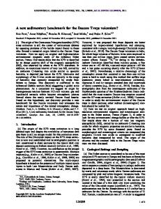
Figure 2: Algorithm performance distributions of the QBF-2011 scenario: Boxplots (left) and cumulative distribution functions (right); both on a log scale. The gaps between the end of the curves (right) and 1.00 denotes the fraction of instances that were not solved within the timeout. • Interesting or challenging properties of the data sets become visible, providing the researcher with a quick and informative first impression. The summary page for the algorithms starts with a table listing simple statistics regarding their performance (e.g., mean values and standard variations) and run status (e.g., how many runs were successful or not). We also indicate whether one algorithm is dominated by another,11 which is useful, because there is no reason to include a dominated algorithm in a portfolio. Various visualizations, such as box plots, scatter plot matrices, correlation plots and density plots enable further inspection of the distribution and correlation between algorithms, allowing the reader to better understand the strengths and weaknesses of each algorithm. For display, we impute high values for the missing performance values corresponding to failed runs so that they are clearly visible rather than silently discarded. All of our plots can be configured to use log scales, which often improves visual understanding when all data are non-negative. Figure 2 shows boxplots and cumulative distribution functions for the algorithms in the QBF-2011 scenario. Such plots allow the detection of mean location, distribution spread, density multimodality and whether the densities are roughly normally distributed. In addition, they reveal how long it took an algorithm to solve the given instances. For example, for the QBF-2011 scenario in Figure 2, one can see that the algorithm quantor finds a solution very quickly on a few instances, i.e., it solves approximately 5% of the instances nearly instantaneously. However, if it does not succeed quickly, it often does not succeed at all—it solved less than 30% of all the instances. In contrast, sSolve usually 11 An algorithm a dominates another algorithm a if and only if a has performance at 1 2 1 least equal to that of a2 on all instances, and a1 outperforms a2 on at least one instance.

14

1e−06

quantor

●

● ● ● ● ● ● ● ● ●●

● ● ● ●

●● ●●●● ● ● ● ●● ● ●● ● ●● ● ● ● ● ● ● ● ● ● ● ● ● ● ● ● ● ● ● ● ●● ●● ● ● ● ● ● ● ● ● ● ● ● ● ● ● ● ● ● ●●● ●● ● ● ● ● ● ● ● ● ● ● ●● ● ● ● ● ● ● ● ● ● ● ● ● ●● ● ● ●● ● ● ● ●● ●● ● ● ● ● ● ●● ● ● ● ● ● ●● ● ●● ● ● ● ● ● ● ● ● ● ● ● ● ● ● ● ● ● ● ● ● ● ● ● ● ● ● ● ● ● ● ● ● ● ● ● ● ● ●● ●● ● ● ●● ●● ●● ●● ● ● ● ● ● ● ● ● ● ● ● ● ● ● ● ● ● ● ● ● ● ● ● ● ● ● ● ● ● ● ● ● ● ● ● ● ●●●● ● ● ● ● ● ● ● ● ● ● ● ● ● ● ● ● ● ● ● ● ● ● ● ● ● ● ● ● ● ● ● ● ● ● ● ●● ● ● ● ● ● ● ● ● ● ● ● ●●

● ● ●

● ● ●● ● ● ● ● ● ● ● ● ●● ● ● ● ● ● ● ● ● ●● ● ● ● ● ● ● ●● ● ● ● ● ● ● ● ● ● ● ● ● ●● ● ● ● ● ● ● ● ● ●● ● ● ● ● ● ●● ● ● ● ● ● ● ● ● ●● ● ● ● ● ● ●● ● ● ● ● ●● ● ● ● ● ● ● ● ● ● ●● ● ● ● ● ● ●● ● ● ● ● ● ● ● ● ● ● ● ● ● ● ● ● ● ● ● ●● ● ● ● ● ● ● ● ● ● ●● ● ● ●●● ● ● ● ● ● ● ● ●● ● ● ● ● ● ● ● ● ● ● ● ● ● ● ● ● ● ● ● ● ● ● ● ● ● ● ● ● ●● ● ● ● ● ● ● ● ● ● ● ● ● ● ● ● ● ● ● ● ● ● ● ● ● ● ● ● ●● ● ● ● ● ● ● ● ● ● ● ● ● ●●● ● ● ● ● ● ● ● ● ● ● ● ● ●● ● ● ● ● ● ● ● ● ● ●●● ● ● ● ● ● ● ● ● ●

● ● ● ●

●●● ● ● ● ● ● ● ●● ● ● ● ● ● ● ● ● ● ● ●● ●● ●● ● ● ● ●● ● ● ●● ● ● ● ● ●● ● ● ● ● ● ●● ● ● ● ● ● ● ● ● ● ● ● ● ● ● ● ● ● ● ● ●● ● ● ● ● ● ● ● ● ● ● ● ● ● ● ● ● ● ● ● ● ● ● ● ● ● ● ● ● ● ● ● ● ● ● ● ● ● ● ● ● ● ● ● ● ● ● ● ● ● ● ● ● ● ● ● ● ●● ● ● ●● ● ● ● ● ● ● ● ● ● ● ● ● ● ● ● ● ● ● ● ● ● ● ● ● ● ● ● ● ● ● ●

●

● ● ● ●●●●● ●● ●●

●

●●●● ● ● ●

●

● ● ●

● ● ●●● ● ● ●● ● ● ● ● ● ● ● ● ● ● ●● ● ● ● ●● ●● ● ● ●● ● ● ● ● ● ● ● ● ● ● ● ● ●●● ● ● ● ● ● ● ● ● ● ● ● ● ● ● ● ●● ● ●● ● ● ● ●● ● ● ● ● ● ● ● ● ●● ● ● ● ●● ● ● ● ● ● ● ● ● ● ● ●● ● ●●● ● ● ● ● ● ● ● ●●● ● ● ● ●● ● ● ● ●● ● ● ● ●●● ● ● ● ● ● ●● ● ● ● ●● ● ● ●● ● ● ● ● ● ● ● ● ● ● ● ● ● ● ● ● ● ● ● ● ● ● ● ● ●● ● ● ● ● ● ● ● ● ● ● ● ● ● ● ● ●● ● ● ● ● ● ● ● ● ● ● ● ● ● ● ● ● ● ●● ● ● ● ● ● ● ● ● ●● ● ● ●● ● ● ● ● ● ● ● ● ● ● ● ● ● ● ● ● ● ● ●

●● ● ● ● ● ● ● ● ● ● ●● ● ● ● ● ● ● ● ● ● ● ● ● ● ●● ● ● ● ● ● ● ● ● ● ● ● ● ●● ● ● ● ● ● ● ● ● ● ● ●● ● ● ● ●●●● ● ● ● ● ● ●● ● ● ● ● ● ●● ●● ●● ● ● ● ● ● ● ● ● ●●●●●● ● ● ● ● ●● ● ● ● ● ●● ●● ●● ● ● ● ● ● ● ● ● ●● ● ●●● ● ●● ● ●● ● ● ● ● ● ● ● ● ● ● ●● ● ● ● ● ● ● ● ● ● ● ● ● ● ● ● ● ● ● ● ● ● ● ● ● ●● ● ● ● ● ● ● ●● ● ● ● ● ● ● ● ● ●● ● ● ● ●● ● ● ●

1e−06

●

1e+02

●

● ● ● ● ● ● ● ● ● ●

● ● ●● ● ● ● ● ● ● ●●● ● ● ● ● ● ● ● ● ● ● ● ● ● ● ● ● ● ● ●● ● ● ● ● ● ● ● ● ● ●● ● ●● ●● ●● ● ● ● ● ● ●● ● ● ● ● ● ● ● ●● ● ●● ● ● ● ● ● ● ●●● ● ● ● ● ● ● ● ● ●● ● ● ● ●● ●●●● ● ● ● ● ● ● ● ● ● ● ● ● ● ● ● ●● ● ● ● ● ● ● ● ● ● ● ● ●● ●● ● ● ● ● ● ●● ● ● ● ● ● ● ● ● ● ● ● ● ●● ● ●●● ● ● ● ● ● ● ● ● ● ● ●● ●●● ● ● ● ● ● ● ● ● ● ● ● ●● ● ● ● ●● ● ● ●

● ● ● ● ●

●● ● ● ● ● ●● ● ● ●●● ● ●●

●

● ●● ● ● ●

● ● ● ● ● ●● ●

● ● ●

●●●● ●● ● ●● ● ● ● ● ● ● ● ● ●● ● ● ●● ● ● ● ● ● ● ●● ● ● ● ● ● ●● ● ● ● ●● ● ●● ● ● ● ● ● ● ● ●● ● ●● ● ● ● ● ● ● ● ● ● ● ● ● ● ● ● ●● ● ● ● ● ● ●● ● ●● ● ● ● ● ●● ● ● ● ● ● ● ● ● ● ● ●● ● ● ● ● ● ● ● ● ● ●● ● ● ● ● ● ● ● ● ● ● ● ● ● ● ● ● ● ● ●● ● ● ● ● ● ● ● ● ● ● ● ● ● ● ● ● ● ● ● ● ● ● ● ● ● ● ●● ● ●● ● ●● ● ● ● ● ● ● ● ● ● ● ● ● ● ● ●● ● ● ● ● ● ● ● ● ● ● ● ● ● ● ● ● ● ● ● ● ● ● ● ● ●●●● ● ● ● ● ●●● ● ● ● ● ● ● ● ● ● ● ● ●● ● ● ● ● ● ●● ● ● ● ●●● ● ● ● ●● ● ● ● ● ● ● ● ● ● ● ●● ● ● ● ●● ● ● ● ● ● ● ● ● ● ● ● ● ● ● ● ● ● ●● ●● ● ● ● ● ● ● ●● ● ● ● ● ● ● ● ● ● ● ● ● ● ● ● ● ● ● ● ●● ● ● ● ● ● ● ● ●● ● ●

● ● ● ● ● ● ● ● ● ●● ● ● ● ● ● ● ●● ● ● ● ● ● ● ● ● ● ● ● ●● ● ●●● ● ● ● ● ●● ●● ● ●● ● ● ●● ● ●● ● ● ● ● ● ● ● ● ● ● ● ● ● ●● ● ●● ● ● ● ● ● ● ● ● ● ●● ● ● ●● ● ●● ● ●●● ● ● ●●● ●● ● ● ● ● ● ●●●● ● ●● ● ● ● ● ● ● ● ● ● ● ● ● ● ● ●● ● ● ● ● ● ● ●● ● ● ● ● ● ● ● ● ● ●● ● ● ● ● ● ● ● ●● ●● ● ● ● ●●●● ● ● ● ● ● ●● ● ● ● ● ● ● ●●● ●● ● ● ● ● ● ● ● ● ● ● ● ● ● ● ● ● ● ● ● ● ● ● ● ● ● ● ● ● ● ● ● ● ● ● ● ● ●● ● ● ● ● ● ● ● ● ● ● ● ● ● ●● ● ● ● ● ● ● ● ● ● ●●●● ● ● ● ● ● ● ● ● ● ● ●● ● ●● ● ● ● ● ● ● ●● ● ●● ● ● ●● ● ● ● ● ●● ● ● ● ● ● ● ● ● ● ● ● ● ●● ● ● ● ● ● ●● ●●●● ● ● ● ● ● ● ● ● ● ● ● ● ● ● ●● ●

●

QuBE

● ● ● ● ● ● ● ● ●

● ●● ● ● ● ● ● ● ● ● ● ● ● ●● ● ● ● ● ● ●● ● ●●● ● ● ● ● ● ● ● ● ● ● ● ● ● ● ● ● ● ● ● ●● ● ● ● ● ● ● ● ● ● ● ● ● ● ● ● ●● ●● ● ● ● ● ● ● ● ● ● ● ● ● ● ● ● ● ● ● ● ● ● ● ● ● ● ● ● ● ● ● ● ● ● ● ●● ● ● ● ● ● ● ● ● ● ● ● ● ● ● ● ● ● ● ● ● ●● ● ● ● ● ● ● ● ● ● ● ● ● ● ● ● ● ●● ● ● ● ● ● ● ● ● ● ● ● ● ● ● ●● ● ● ● ● ● ● ● ● ● ● ● ● ● ● ● ● ● ● ● ● ● ● ●● ● ●● ● ●● ●● ● ● ● ● ● ● ● ● ● ● ● ● ● ● ● ●● ● ● ● ● ● ● ● ● ●●● ● ● ● ● ● ● ● ● ● ● ● ● ● ● ● ● ● ● ● ● ● ● ● ● ● ● ● ● ● ● ●● ● ● ● ● ● ● ● ● ● ● ● ● ●● ● ● ● ● ● ● ● ● ● ● ● ● ● ● ●● ● ● ● ●● ● ● ● ● ●● ●● ● ● ● ● ● ● ● ● ● ●●● ● ● ● ● ● ● ● ● ● ● ● ● ● ● ●

●● ● ● ● ● ●● ● ● ●

●● ●

● ● ● ● ● ● ●● ● ● ● ● ● ● ● ● ●● ● ● ● ● ●● ● ● ● ● ●● ● ● ● ● ● ● ● ● ● ● ● ● ●● ● ● ● ●● ● ● ●●● ● ● ● ● ● ● ● ● ●● ● ● ● ● ● ● ● ●● ● ● ●● ● ● ● ● ● ● ●● ● ● ● ● ● ● ● ● ●●● ● ● ● ● ● ● ●●● ● ● ● ●● ● ●● ●● ● ● ● ● ● ● ●● ● ● ● ● ● ● ● ● ● ● ● ●● ● ● ● ● ● ● ● ●●● ● ● ● ● ● ● ●● ● ● ● ● ● ●● ●● ● ●●● ● ●● ● ● ● ● ● ● ● ● ● ● ●● ● ● ●● ● ● ●●● ● ● ● ● ● ● ●● ● ● ● ●● ● ● ● ● ● ●●●● ● ● ●● ● ● ● ● ● ● ● ● ● ● ● ● ● ● ● ● ● ● ●● ● ● ● ● ● ● ● ● ● ●● ●● ● ● ● ● ● ● ●● ● ● ● ● ● ● ● ● ● ● ● ● ● ● ● ● ● ● ● ●● ● ●● ● ● ●● ● ● ● ● ● ● ● ● ● ● ● ● ● ● ● ● ● ● ● ● ● ● ● ● ●● ● ● ●● ●● ●● ● ● ● ● ● ●

1e−01

sKizzo

●● ●

1e+03

●

● ● ● ●

1

quantor

sKizzo

0 −0.2

X2clsQ

−0.4

●

sSolve 1

0.4 0.2

sSolve

● ● ● ● ● ● ● ● ● ● ●● ● ● ●● ● ● ● ● ● ●● ● ● ●● ● ● ● ● ● ● ●●● ● ● ● ●● ● ● ● ● ● ● ● ● ● ● ● ● ● ● ● ●● ● ● ● ● ● ● ● ● ● ● ● ● ● ● ● ● ● ●●● ● ● ● ● ● ● ● ● ● ● ●●●●● ● ● ●●● ● ● ● ●● ●● ● ● ●● ● ● ● ● ● ● ● ● ● ●● ● ● ●● ● ● ● ● ● ● ● ● ● ● ●● ● ● ● ● ● ● ● ● ●● ● ●● ●● ●● ● ● ● ● ● ● ● ● ● ● ● ● ● ● ● ● ● ● ● ● ●● ● ●● ● ● ● ●●●● ● ● ● ●● ● ● ● ● ● ● ● ● ● ● ● ● ●● ● ● ● ● ● ● ● ●● ● ●● ● ●● ● ● ● ● ● ● ● ● ● ● ● ●● ● ● ● ● ● ● ● ● ● ● ●● ● ●● ● ● ●● ● ● ●● ●● ● ● ● ● ● ● ● ● ● ● ● ● ● ● ● ● ● ● ● ● ● ● ● ● ● ● ● ● ● ● ● ● ● ● ● ● ● ● ● ● ● ●

●● ● ●● ● ● ● ● ● ● ● ●● ● ● ● ●● ● ●● ● ● ● ● ● ●● ● ● ● ● ● ●● ● ● ● ● ●● ● ● ● ● ● ● ● ● ●● ● ●● ● ● ● ● ● ● ● ● ● ● ●● ● ●● ● ● ● ● ● ● ● ● ● ● ● ● ● ● ● ● ●●● ●● ●●● ●●●● ● ● ● ● ● ●● ● ● ● ● ● ● ●● ●● ● ● ● ● ● ● ●● ● ● ● ● ● ● ● ● ● ● ● ● ● ●● ●● ● ●● ●● ● ● ● ● ● ● ● ●●● ● ● ● ● ● ● ● ● ● ● ● ● ● ●● ● ● ● ● ● ● ●●● ● ● ● ● ● ● ● ● ● ●● ●● ● ● ● ● ● ● ● ● ● ● ● ● ● ● ● ● ● ● ● ●● ● ● ●●●●● ● ● ●● ● ● ●● ● ● ● ● ● ● ● ● ● ● ● ● ● ● ● ● ● ● ● ● ● ● ● ● ● ● ● ● ● ● ● ● ●● ● ● ● ● ● ● ● ● ● ● ● ● ● ● ● ● ● ● ● ● ● ● ● ● ● ● ● ●● ● ●● ●● ● ● ● ● ● ● ● ● ●

0.8 0.6

●

● ● ● ● ● ● ●● ● ●

QuBE

● ●● ● ● ● ● ● ● ● ● ● ● ●● ● ● ● ● ●● ● ● ● ● ● ● ● ● ● ● ● ●● ● ● ● ● ● ● ● ● ● ● ● ●● ● ●● ● ● ●● ● ●● ● ● ● ● ● ● ● ● ● ● ● ● ● ● ● ● ●● ●● ● ● ● ● ● ● ● ● ● ●● ● ● ● ● ● ● ● ● ● ● ● ● ● ●● ● ● ● ● ● ● ● ● ● ●● ● ●● ● ● ● ● ● ● ● ● ● ● ● ● ●● ●● ● ● ● ● ● ● ● ● ● ● ●● ●● ●● ● ● ● ● ● ● ●● ● ● ● ● ● ● ● ● ● ● ● ● ● ● ● ● ● ● ● ●●●● ●● ● ● ● ● ● ● ● ● ● ● ● ● ● ● ● ●●● ● ● ● ● ● ● ● ● ● ● ● ● ● ● ● ● ● ● ●

X2clsQ

● ● ● ● ● ●

●● ● ●● ● ● ● ● ● ● ● ● ● ● ● ● ●● ● ● ● ● ● ●● ● ● ● ● ● ● ● ●● ● ●● ● ● ● ● ● ● ● ● ● ●● ● ● ●● ● ● ● ● ● ● ● ● ● ● ● ● ● ●● ● ● ● ● ● ● ● ● ● ● ● ● ● ● ● ●● ● ● ● ● ● ●● ● ● ● ● ● ● ● ● ● ● ●● ● ● ● ● ● ● ●● ● ● ●● ● ●● ● ● ● ● ● ● ● ● ● ● ● ● ● ● ●● ● ● ● ● ● ● ● ● ● ● ● ● ● ● ● ● ● ● ● ● ● ● ●● ● ● ● ● ● ● ● ● ● ● ● ● ● ● ● ● ● ● ● ● ● ● ● ● ● ● ● ● ●● ● ● ● ● ● ● ● ●● ● ●

sSolve

● ● ●

● ● ● ● ● ● ●

sKizzo

●

●● ● ● ● ● ● ●● ● ● ● ● ●● ● ●● ● ● ● ●● ● ● ● ● ● ●● ● ● ● ● ● ● ●● ● ●●● ● ● ● ● ● ● ●● ● ● ● ● ● ● ● ● ● ● ● ● ● ●● ● ● ● ● ● ● ● ● ● ● ● ● ● ● ● ● ● ● ● ● ● ● ● ● ● ● ● ● ●● ● ● ● ● ● ● ● ● ●● ●● ●● ● ● ● ● ●● ● ● ● ● ● ● ● ● ● ● ● ● ● ● ●●●● ●● ● ● ●● ●● ● ● ● ● ● ● ● ● ● ●●●● ● ● ● ●● ● ● ● ● ●● ● ● ● ●● ● ● ●● ● ●● ● ● ● ● ● ●● ● ● ● ● ●● ● ● ● ● ● ●● ● ● ● ● ● ●● ●● ●● ● ● ● ● ● ● ● ● ●● ● ● ●● ● ● ● ●● ● ● ● ● ● ● ● ● ● ● ●

quantor

●● ●● ● ● ● ● ●

1e+02

●

● ● ● ● ● ● ● ● ● ● ● ● ● ● ● ●● ● ● ● ● ● ● ● ● ● ● ● ● ● ●● ● ●● ● ● ● ● ● ● ● ●● ● ●● ● ● ●● ● ●● ● ● ● ● ● ● ● ● ● ● ● ● ● ● ●● ● ●● ● ● ● ● ● ● ● ● ● ● ● ● ● ● ● ● ● ● ● ● ● ● ● ● ● ● ●● ● ● ● ● ● ● ● ● ● ● ● ● ● ● ● ● ● ● ● ● ● ●● ● ● ● ● ● ● ●●● ● ● ● ●● ● ● ● ● ●●● ● ●● ● ● ● ● ● ● ●● ● ● ● ● ● ● ●● ● ● ● ● ● ● ● ●● ● ● ● ●●●● ● ● ● ● ● ● ● ● ● ● ● ● ● ●● ● ● ● ● ● ● ● ● ● ● ● ● ●● ●●● ● ● ● ● ● ●● ● ● ● ● ● ● ● ● ● ● ● ● ● ● ● ● ● ● ● ● ● ● ● ● ● ● ● ● ● ● ● ● ● ● ● ● ● ● ● ● ●● ●●●● ● ●

1e−06

●

●●●● ●● ● ●● ● ● ● ● ● ● ● ● ●● ● ● ●● ● ● ● ● ● ● ● ●● ● ● ● ● ●● ● ● ● ● ●● ● ●● ● ● ● ● ● ● ● ● ●● ● ● ●● ● ● ● ● ● ● ● ● ● ● ● ● ● ● ● ● ● ● ● ● ● ● ● ● ● ● ● ● ● ● ● ● ● ● ● ● ● ● ● ● ●● ●● ● ● ● ● ● ● ● ● ● ● ● ●● ● ● ●● ● ● ● ● ● ● ● ● ● ●●● ● ● ● ● ● ● ● ● ● ● ● ● ● ● ● ● ● ● ● ● ● ● ● ● ● ● ● ● ● ● ● ●● ● ● ● ● ● ● ● ● ●● ● ● ● ● ● ● ●● ● ● ● ● ● ● ● ● ● ● ● ● ● ● ● ● ● ● ● ● ● ● ● ● ● ● ● ● ●● ●● ●● ● ● ● ● ● ● ● ● ● ● ● ● ● ● ● ● ● ●● ● ● ● ● ● ● ● ● ● ● ● ● ● ● ● ● ● ● ● ● ● ● ● ● ● ● ● ● ● ● ● ● ● ● ●

1e+03

● ● ● ● ● ●● ● ● ● ● ● ● ● ● ●● ● ● ● ● ●● ● ●● ●● ● ● ● ●● ● ● ● ●●● ● ●● ● ● ● ● ● ●● ● ●● ● ●● ● ●● ● ● ● ● ● ● ● ● ● ● ● ●●● ● ● ● ● ●● ● ● ● ●●● ● ●●●● ● ● ● ● ● ● ● ● ● ●● ● ●● ● ● ● ● ● ● ●● ● ● ● ● ● ● ●●● ● ● ● ● ● ● ● ● ● ● ● ● ● ● ● ● ● ●● ● ● ●● ● ● ● ● ● ● ● ●● ● ● ● ● ● ●● ● ● ● ● ● ● ● ● ●● ● ● ● ●●● ● ● ●● ●● ● ● ● ● ● ● ● ●

1e+02

● ● ● ● ● ● ● ● ● ●

1e−01

● ● ● ●

1e−06 ● ● ● ● ● ● ●● ●● ● ● ● ● ●● ● ● ● ● ●● ● ●●● ● ● ● ● ● ● ●● ● ● ●● ● ● ● ● ●● ● ● ● ● ● ● ● ● ● ● ● ● ● ● ● ● ● ● ● ● ● ● ● ● ● ● ● ● ● ● ● ● ● ● ● ● ● ● ● ● ● ● ● ●● ● ● ● ● ● ● ● ● ●● ● ●● ● ● ● ● ● ● ● ● ●● ● ● ● ● ●● ● ● ● ● ● ● ●● ● ● ● ●● ● ● ● ● ● ● ● ● ● ● ● ●● ● ●● ● ● ● ●● ● ● ● ● ● ● ● ● ● ● ● ●● ● ● ● ● ● ● ●● ●● ●● ● ● ● ● ● ● ● ● ● ● ● ● ●● ● ● ● ● ● ● ● ● ● ● ● ● ● ● ● ● ● ● ● ● ● ● ● ● ● ● ● ● ● ● ●● ● ● ● ● ● ● ● ● ● ● ● ● ● ● ● ● ● ● ● ● ●● ● ● ● ● ● ●● ●●● ● ● ● ● ● ● ● ● ● ● ● ● ● ● ● ● ● ● ● ●●● ● ● ● ● ● ● ● ● ● ● ● ● ● ● ● ● ●●

5000

●

1e+02

1e−06

1e+02

X2clsQ

1e+02 ● ● ● ● ● ● ● ● ● ● ● ● ● ● ● ● ● ● ● ● ●● ● ● ● ● ● ● ● ● ●● ● ● ● ● ● ● ●●●● ● ● ●●●● ● ● ● ● ● ● ● ● ●● ● ●● ● ●● ● ●● ● ● ● ● ●● ● ●●● ● ● ● ● ● ● ● ● ● ● ● ●● ● ● ● ●● ● ● ● ● ● ● ● ● ● ● ● ● ● ● ●● ● ● ● ●● ● ● ● ● ● ● ● ● ● ● ● ● ● ● ● ● ● ● ● ● ● ● ● ● ● ● ● ● ● ● ● ● ● ●● ●● ● ● ● ● ● ● ● ●● ●

● ● ● ●

50

●

1

1e−06

50

−0.6

QuBE

−0.8 −1

5000

Figure 3: Pairwise correlations among algorithms of the QBF-2011 scenario: A scatter plot matrix on a log scale (left) and the plot of a clustered correlation matrix (right). needs longer to find a solution, but by the time it does, it is one of the best algorithms. Such behavior can indicate that the algorithm requires a ‘warm-up’ stage, which should be considered when deploying it. The left panel of Figure 3 shows pairwise scatterplots of the QBF-2011 scenario, allowing an easy comparison of algorithm pairs on all instances from a given scenario. Each point represents a problem instance within the task, and from the location of the point cloud, one can see whether an algorithm is dominant over the majority of instances, or whether relative performance strongly varies between instances. The first case can be identified by a cloud that is located either in the upper-left or lower-right corner of a single scatterplot. In such a case, the dominated algorithm could be discarded from the portfolio. However, if this type of domination is not present, there is the potential to realize performance improvements by means of per-instance algorithm selection. Because detecting correlation in algorithm performance is also of interest when analyzing the strengths and weaknesses of a given portfolio-based solver [106], we also present a clustered correlation matrix, cf. Figure 3 (right panel). Algorithms that have a (high) positive correlation are more likely to be redundant in a portfolio, whereas pairs with a (high) negative correlation are more likely to complement each other. Here, we calculate Spearman’s correlation coefficient between ranks. Blue boxes represent positive correlation, red boxes represent negative correlation, and shading indicates the strength of correlation. The algorithms are also clustered according to these values (using Ward’s method [100]) and then sorted, such that similar algorithms appear together in blocks. This

15

minisatpsm rcl ebglucose glucose2 qutersat cryptominisat2011 lrglshr glueminisat lingeling precosat sol spear−sw spear−hw clasp2 clasp1 mxc09 picosat sapperlot ebminisat restartsat sattimep satime11 sattime eagleup gnoveltyp2 sparrow tnm marchrw mphaseSAT64 mphaseSATm mphaseSAT

1

minisatpsm rcl ebglucose glucose2 qutersat cryptominisat2011 lrglshr glueminisat lingeling precosat sol spear−sw spear−hw clasp2 clasp1 mxc09 picosat sapperlot ebminisat restartsat sattimep satime11 sattime eagleup gnoveltyp2 sparrow tnm marchrw mphaseSAT64 mphaseSATm mphaseSAT

0.8

0.6

0.4

0.2

0

−0.2

−0.4

−0.6

−0.8

−1

Figure 4: Clustered correlations for the SAT12-ALL scenario. type of clustering allows the identification of algorithms with highly correlated performance. The example given in Figure 4 (the plot of a correlation matrix of the SAT12ALL scenario) shows three groups of algorithms (minisatpsm to restartsat, sattimep to tnm and the three mphaseSAT -algorithms) with high correlations within each group. Also, the performance of marchrw is distinct from all the others. Hence, one might want to select a representative per group, reducing the size of the entire portfolio from 31 to four algorithms. As we do with algorithm runs, we summarize the features e.g., by giving basic statistics of the feature values, and the run status and cost of the feature processing steps. Table 3 displays the summary of the feature steps for the SAT12-RAND scenario. In this scenario, all 115 features use the feature step ‘Pre’ as a requirement (since the first step is to preprocess the instance). While

16

runstatus [%]

cost [s]

feature step

#

ok

...

crash

min

mean

max

missing [%]

Pre Basic KLB CG DIAMETER cl sp ls saps ls gsat lobjois

115 14 20 10 5 18 18 11 11 2

100.00 100.00 100.00 62.63 100.00 100.00 100.00 100.00 100.00 100.00

... ... ... ... ... ... ... ... ... ...

0.00 0.00 0.00 37.37 0.00 0.00 0.00 0.00 0.00 0.00

0.00 0.00 0.00 0.02 0.00 0.01 0.01 1.36 2.03 2.00

0.06 0.00 0.18 8.79 0.60 1.99 0.33 2.12 2.29 2.00

1.31 0.07 6.09 20.28 2.11 2.02 3.05 2.51 3.03 2.27

0.00 0.00 0.00 0.00 0.00 0.00 0.00 0.00 0.00 0.00

Table 3: Feature group summary for the SAT12-RAND scenario. The second column shows how many features depend on a feature group as a requirement; next, proportions of runstatus events are listed, followed by basic statistics for step costs. this preprocessing step succeeded in all cases, one other step did not: the feature step ‘CG’ (which computes clause graph features) failed in 37.37% of cases due to exceeding time or memory limits, and even for instances where it succeeded, it was quite expensive (8.79 seconds on average). Such information is useful understanding feature behavior: e.g., how risky it is to compute a feature step; how much time must one invest in order to obtain the corresponding features? We also check whether instances occur with exactly the same feature values, indicating that the experimenter might have erroneously run on the same instance twice. It should be mentioned that all of the tables and figures presented, and additional ones, which we have omitted for space reasons, were automatically generated by our online platform, and are also accessible through the R package aslib. The functions are highly configurable, so users can use them for their own data exploration or publications and flexibly combine individual elements. For the future, we plan to extend our data analysis by additional techniques, such as further measures of algorithm performance [82]. 6. Basic Algorithm Selection Experiments In this section, we present exploratory benchmark experiments that give an indication of the diversity of our benchmarks. First, we evaluate the performance of basic algorithm selectors on our scenarios. We then perform a subset selection study to identify the important algorithms and instance features in each of the scenarios. We make no claim that the presented experimental settings are exhaustive or that we achieve state-of-the-art algorithm selection performance; rather, we provide baseline results that can be achieved by standard machine learning approaches for the core technology of an algorithm selection system—the 17

selector itself. These results, and our framework in general, allow us to study which algorithm selection approaches work well for which of our scenarios. In order to reach the performance of current state-of-the-art algorithm selection systems [64, 107], we would have to include various extensions, such as cost-sensitive classification and complementary techniques such as pre-solving.12 We use the LLAMA toolkit [53], version 0.8.1, in combination with the aslib package13 to run the algorithm selection experiments. LLAMA is an R [75] package that facilitates many common algorithm selection scenarios. In particular, it enables access to classification, regression, and clustering models for algorithm selection—the three main approaches we use in our experiments—from other R packages. As LLAMA does not include any machine learning algorithms, we use the mlr R package [12] as an interface to the machine learning models provided by other R packages. We parallelize all of our benchmark experiments through the BatchExperiments [11] R package. In this paper, we only present aggregated benchmark results, but the interested reader can access full benchmark results at http://aslib.net. Our experiments are fully reproducible as the complete code to generate these results can be accessed in the Github repository mentioned earlier. Please note that for some of the algorithm selection scenarios we have opted to use only a subset of feature processing groups (and their associated features) as recommended by authors of the scenarios; we did this because some feature steps are excessively expensive to calculate and have not fully proved their worth in selection models. Detailed information (e.g., the names of the feature processing groups we selected and their average costs) is provided on the ASlib webpage. 6.1. Data preprocessing Before running the experiments, we preprocessed the training data as follows. We removed constant-valued (and therefore irrelevant) features and imputed missing feature values as the mean over all non-missing values of the feature. We normalized the range of each feature to the interval [−1, 1]. While this is unnecessary for some machine learning approaches (e.g., decision trees), it is often helpful or mandatory for others (e.g., SVMs or clustering). Missing performance values were imputed using the timeout value for the data set. For each problem instance, we calculated the feature computation cost based on the costs for the feature groups specified in the data. If the problem instance was solved during feature computation, we only considered the cost of the features up to the one that solved it. Furthermore, we set the runtime for all algorithms to zero for instances solved during feature computation. We added the feature 12 A pre-solver is a default solver that is run for a small amount of time without any algorithm selection taking place; cf. [104]. The problem instances that are solvable in this time are solved without incurring any of the overhead that algorithm selection brings, such as the computation of features. This is relevant in practice, as the cost of computing features can be much higher than the cost of solving a very easy instance. 13 https://github.com/coseal/aslib-r

18

costs computed in this way to the runtimes of the individual algorithms on the respective instances. Given these new runtimes, we checked whether the specified timeout was now exceeded by any algorithm and set the run status of the corresponding algorithm accordingly. Preprocessing runtimes to include feature computation time in this way allows us to focus on an algorithm selection system’s overall performance, and avoid overstating the fraction of instances that would be solved within a time budget in cases where features are expensive to compute. Each scenario specifies a partition into 10 folds for cross-validation to ensure consistent evalution across different methods. We also used this splitting in our experiments. 6.2. Experimental setup We consider three fundamentally different approaches to algorithm selection that have been studied extensively in the literature (cf. Section 2.2): • classification: using a multi-class classifier to directly predict the best of the k possible algorithms; • regression: predicting each algorithm’s performance via a regression model and then choosing the one with the best predicted performance; • clustering: clustering problem instances in feature space, then determining the cost-optimal solver for each cluster and finally assigning each new instance to the solver associated with the instance’s predicted cluster. Technical Name classification ksvm randomForest rpart regression lm randomForest rpart clustering XMeans

Algorithm and parameter ranges

reference

support vector machine C ∈ [2−12 , 212 ], γ ∈ [2−12 , 212 ] random forest ntree ∈ [10, 200], mtry ∈ [1, 30] recursive partitioning tree, CART

[49]

linear regression random forest ntree ∈ [10, 200], mtry ∈ [1, 30] recursive partitioning tree, CART

[75] [60] [91]

extended k-means clustering

[33]

[60] [91]

Table 4: Machine learning algorithms and their parameter ranges used for our experiments. The specific machine learning algorithms we employed for our experiments are shown in Table 4. To provide a good baseline, they include representatives from 19

each of the three major approaches above. We tuned the hyperparameters of ksvm and randomForest (classification and regression) with the listed parameter ranges, using random search with 250 iterations and a nested cross validation (with 3 internal folds) to ensure unbiased performance results. All other parameters were left at their default values. For the clustering algorithm, we set the (maximum) number of clusters to 30 after some preliminary experiments; the exact number of clusters was determined dynamically by XMeans. 6.3. Evaluation Each of the algorithm selection models was evaluated based on three different measures: the fraction of all instances solved within the timeout; the penalized average runtime with a penalty factor of 10 (PAR10: this means averaging runtimes with timeouts counting as 10 times the time budget); and the average misclassification penalty (which, for a given instance, is the difference between the performance of the selected algorithm and the performance of the best algorithm). The performance of each algorithm selection model was compared to the virtual best solver (VBS) and the single best solver. Note that the misclassification penalty for VBS is zero by definition. The single best solver is the (actual) solver that has the overall best performance on the data set. Specifically, we consider the solver with the best PAR10 score over all problem instances in a scenario.14 6.4. Experimental results Figure 5 presents a summary of our experimental results. In most cases, the algorithm selection approaches performed better than the single best solver. We expected this, as all of our data sets came from publications that advocated algorithm selection systems. Nevertheless, there were significant differences between the scenarios. While for most of them, almost all algorithm selection approaches outperformed the single best algorithm, there are some scenarios that seem to be much harder for algorithm selection. In particular, on the SAT11-INDU scenario, three approaches were not able to achieve a performance improvement and all other approaches (with the exception of random regression forests) improved only slightly. Random regression forests stood out as quite clearly the best overall approach, yielding the best performance for 11 of the 13 datasets. This is in line with recent results showing the strong performance of this model for algorithm runtime prediction [45]. The results are also consistent with those of the original papers introducing the datasets. For example, Xu et al. [106] reported somewhat better results for the three SAT11 datasets than the one achieved here with our off-theshelf methods (which is to be expected since their latest SATzilla version used a cost-sensitive approach and pre-solving schedules). 14 The single best solvers determined according to the other evaluation measures described here are presented in the detailed experimental results on the ASlib web page; the results were qualitatively similar.

20

0.63 0.46 0.03 0.31 −0.20 −0.26 0.91 0.74 0.80 0.75 0.35 −0.02 0.80 0.37 0.07 0.45 −0.02 −0.24 0.08 −0.26 0.32 0.89 0.70 0.46 0.86 0.62 0.60 0.86 0.32 0.23 0.81 0.71 0.50 0.77 0.53 0.37 0.21 0.20 0.18 t

ea r/X M

/rp gr cl

us

te

re

Fo r nd

ar

es

/lm gr re /ra

m do si f/r an

om

t es Fo r

ks if/ ss

0.63 0.31 0.91 0.75 0.80 0.45 0.32 0.89 0.86 0.86 0.81 0.77 0.35

cl

as

cl a

0.23

ns

0.44 0.03 0.81 0.57 0.64 0.32 0.08 0.71 0.63 0.66 0.77 0.55 0.16

t

0.53 0.04 0.87 0.17 0.35 −0.34 0.26 0.72 0.62 0.83 0.47 0.47 0.35

vm

0.58 0.02 0.87 0.71 0.67 0.42 −0.08 0.79 0.65 0.61 0.74 0.35 0.19

gr

ASP−POTASSCO PREMARSHALLING−ASTAR−2013

0.35

re

CSP−2010 PROTEUS−2014

0.61 −0.03 0.79 0.64 0.61 0.20 0.10 0.70 0.76 0.75 0.74 0.39 0.27

rt

QBF−2011 MAXSAT12−PMS

0.64

pa

SAT12−INDU SAT12−RAND

0.49

f/r

SAT12−ALL SAT12−HAND

0.41

si

SAT11−RAND

0.50

as

SAT11−INDU

0.50

cl

SAT11−HAND

Figure 5: Summary of the experimental results. We show how much of the gap between the single best and the virtual best solver in terms of PAR10 score was closed by each model. That is, a value of 0 corresponds to the single best solver and a value of 1 to the virtual best. Negative values (highlighted in italics) indicate performance worse than the single best solver. Within each data set, the best model is highlighted in bold italics. The shading emphasizes that comparison: dark cells correspond to values close to 1 (i.e. close to the virtual best solver), whereas lighter fillings correspond to the worse models. Above the heatmap, the arithmetic mean is given for each model type across all scenarios, allowing for a quick comparison of the different models. The numbers on the right-hand side of the heatmap show the best performance for each scenario. XMeans performed worst on average. We suspect that the performance of clustering approaches is highly sensitive to the selection and normalization of instance features. On some scenarios, XMeans performed well; it was the best-performing approach on SAT12-RAND. However, on SAT11-INDU, SAT12INDU, and SAT12-ALL (which also partly consists of industrial SAT instances), XMeans performed worse than the single best solver. This leads us to suspect suspect that the default subset of instance features is not favorable for XMeans on industrial SAT instances. 6.5. Algorithm and Feature Subset Selection To provide further insights into our algorithm selection scenarios, we applied forward selection [52] to the algorithms and features to determine whether smaller subsets still achieve comparable performance. We performed forward search independently for algorithms and features for each scenario. 21

The process starts with the empty set and then greedily and iteratively adds the algorithm or feature to the set which most improves the cross-validated score (PAR10) of the predictor. The selection is terminated when the score does not improve by at least 1. In all other aspects, the experimental setup was the same as described before. As a prognostic model we used the random regression forest,15 as it was the best overall approach so far. We note that the selection results use normal resampling and not the nested version, which may result in overconfident performance estimates for the selected subsets [14]. We accept this caveat since our goal here is to study the ranking of the features and the size of the selected sets, and a more complex, nested approach would have resulted in multiple selected sets.

Scenario SAT11-HAND SAT11-INDU SAT11-RAND SAT12-ALL SAT12-HAND SAT12-INDU SAT12-RAND QBF-2011 MAXSAT12-PMS CSP-2010 PROTEUS-2014 ASP-POTASSCO PREMARSHALLINGASTAR-2013

Original (tuned) PAR10

Algorithms

Features

Number

PAR10

Number

PAR10

17897.90 12598.37 10173.51 943.20 4204.49 2792.21 3239.43 9074.97 3367.55 6466.71 5858.31 509.12 5546.52

15 → 7 18 → 5 9→4 31 → 15 31 → 8 31 → 7 31 → 3 5→4 6→4 2→2 22 → 7 11 → 8 4→3

16404.70 12295.47 9947.35 924.72 4342.31 2770.48 3135.41 9149.56 3274.20 6494.05 5734.79 496.93 5439.27

113 → 5 112 → 5 112 → 5 113 → 5 113 → 5 113 → 4 113 → 3 46 → 8 30 → 4 69 → 3 31 → 3 134 → 3 16 → 4

15913.69 10787.97 9775.63 866.03 4076.52 2537.77 3079.54 8895.07 3249.77 6391.16 5894.08 481.75 4407.74

Table 5: Number of selected algorithms and features and the resulting PAR10 values for the corresponding reduced sets. For reference, the second column lists the PAR10 score of the regression forest on the full algorithm and feature sets from the previous set of experiments.

Table 5 presents the results of forward selection for algorithms and features on all scenarios. Usually, the number of selected features is very small compared to the complete feature set. This is consistent with the observations of Hutter et al. (2013) who showed that only a few instance features are necessary to reliably predict the runtime of algorithm configurations. For example, on SAT12-RAND, the only three features selected were a feature based on survey propagation concerning the probability of variables to be unconstrained, and two balance 15 We used the random forest with default parameters, as the tuning was done for the full set of features and solvers.

22

features concerning the ratio of positive and negative (1) occurences of each variable and (2) literals in each clause. The number of algorithms after forward selection is also substantially reduced on most scenarios. On the SAT scenarios, we expected to see this because the scenarios consider a huge set of SAT solvers that were not pre-selected in any way. Xu et al. (2012a) showed that many SAT solvers are strongly correlated (see Figure 4 in Section 5) and make only very small contributions to the VBS. For example on the SAT12-RAND scenario, only three solvers were selected: sparrow, eagleup, and lingeling. We did not expect the set of algorithms to be reduced on the ASP-POTASSCO scenario, as the portfolio was automatically constructed using algorithm configuration to obtain a set of complementary parameter settings that are particularly amenable to portfolios; indeed, forward selection kept as many as 8 of the 11 configurations. Our results indicate that in real-world settings, selecting the most predictive features and the solvers that make the highest contributions can be important. More detailed results can be found on the ASlib website. 7. Conclusion We have introduced ASlib, a benchmark library for algorithm selection, a rapidly growing field of research with substantial impact on various subcommunities in artificial intelligence. Release version 1.0.1 of the library comprises 12 algorithm selection scenarios from six different areas with a focus on (but not a limitation to) constraint satisfaction problems. We discussed the format of new algorithm selection scenarios and showed examples of the automated exploratory data analysis that will run for each new scenario submitted to our online platform http://aslib.net/. Finally, exploratory experiments with various simple types of algorithm selection systems on our 12 algorithm selection scenarios demonstrated that even simple algorithm selection systems can dramatically outperform the single best solver and confirmed that random forest models performed best overall. We achieved performance improvements over the best single solver on all data sets, often reducing penalized average runtime by a factor of 2 and in the best case by a factor of 3. ASlib facilitates research on algorithm selection methods by providing a common set of benchmarks and tools for working with these. Similar to solver competitions, it enables principled comparative empirical performance assessment. It also considerably lowers the otherwise rather high barrier for researchers to work on algorithm selection, since anyone using the benchmark scenarios we provide does not have to perform actual runs of the solvers contained in them. Since our library provides performance data for the solvers and problem instances included in each selection scenario (which otherwise would have to be produced, at considerable computational cost, by anyone working with that scenario), using ASlib also substantially reduces the computational burden of performance assessments. The carefully selected set of scenarios included in release version 1.0.1 of ASlib challenge algorithm selection methods in various ways and thus provide a solid basis for developing and assessing such methods. 23

Future updates will ensure that ASlib remains useful as research on algorithm selection progresses. Acknowledgements We thank the creators of the algorithms and instance distributions used in our various algorithm selection scenarios. The performance of algorithm selection systems depends critically upon the ingenuity and tireless efforts of domain experts who continue to invent novel solver strategies. References [1] Ans´otegui, C., Malitsky, Y., Sellmann, M., 2014. MaxSAT by Improved Instance-Specific Algorithm Configuration, in: Proceedings of the TwentyEighth National Conference on Artificial Intelligence (AAAI’14), pp. 2594– 260. [2] Ans´otegui, C., Sellmann, M., Tierney, K., 2009. A gender-based genetic algorithm for the automatic configuration of algorithms, in: Proceedings of the Fifteenth International Conference on Principles and Practice of Constraint Programming (CP’09), pp. 142–157. [3] Arbelaez, A., Hamadi, Y., Sebag, M., 2010. Continuous search in constraint programming, in: Proceedings of the Twenty-Second IEEE International Conference on Tools with Artificial Intelligence, pp. 53–60. [4] Argelich, J., Berre, D.L., Lynce, I., Marques-Silva, J., Rapicault, P., 2010. Solving linux upgradeability problems using boolean optimization, in: Proceedings of the International Workshop on Logics for Component Configuration, pp. 11–22. [5] Argelich, J., Li, C., Many`a, F., Planes, J., 2012. Seventh MaxSAT Evaluation. http://www.maxsat.udl.cat/12/. [6] Baral, C., 2003. Knowledge Representation, Reasoning and Declarative Problem Solving. Cambridge University Press. [7] Biere, A., 2014. Yet another local search solver and Lingeling and friends entering the SAT competition 2014, in: Proceedings of SAT Competition 2014: Solver and Benchmark Descriptions, pp. 39–40. [8] Biere, A., Heule, M., van Maaren, H., Walsh, T. (Eds.), 2009. Handbook of Satisfiability. volume 185 of Frontiers in Artificial Intelligence and Applications. IOS Press. [9] Birattari, M., Yuan, Z., Balaprakash, P., St¨ utzle, T., 2010. in: Empirical Methods for the Analysis of Optimization Algorithms. Springer. chapter F-race and iterated F-race: An overview.

24

[10] Bischl, B., Kotthoff, L., Lindauer, M., Malitsky, Y., Frech´ette, A., Hoos, H., Hutter, F., Kerschke, P., Leyton-Brown, K., Vanschoren, J., 2014. Algorithm Selection Format Specification. Technical Report. Available at http://www.aslib.net/. [11] Bischl, B., Lang, M., Mersmann, O., Rahnenf¨ uhrer, J., Weihs, C., 2015a. BatchJobs and BatchExperiments: Abstraction mechanisms for using R in batch environments. Journal of Statistical Software 64, 1–25. [12] Bischl, B., Lang, M., Richter, J., Bossek, J., Judt, L., Kuehn, T., Studerus, E., Kotthoff, L., 2015b. mlr: Machine Learning in R. R package version 2.3. https://github.com/berndbischl/mlr. [13] Bischl, B., Mersmann, O., Trautmann, H., Preuss, M., 2012a. Algorithm selection based on exploratory landscape analysis and cost-sensitive learning, in: Proceedings of the Fourteenth Annual Conference on Genetic and Evolutionary Computation, pp. 313–320. [14] Bischl, B., Mersmann, O., Trautmann, H., Weihs, C., 2012b. Resampling methods for meta-model validation with recommendations for evolutionary computation. Evolutionary Computation 20, 249–275. [15] Brazdil, P., Giraud-Carrier, C., Soares, C., Vilalta, R., 2008. Metalearning: Applications to Data Mining. 1 ed., Springer Publishing Company, Incorporated. [16] Cicirello, V.A., Smith, S.F., 2005. The max k-armed bandit: A new model of exploration applied to search heuristic selection, in: Proceedings of the Twentieth National Conference on Artificial Intelligence, AAAI Press. pp. 1355–1361. [17] Cook, D.J., Varnell, R.C., 1997. Maximizing the benefits of parallel search using machine learning, in: Proceedings of the Fourteenth National Conference on Artificial Intelligence, AAAI Press. pp. 559–564. [18] Crawford, J.M., Baker, A.B., 1994. Experimental results on the application of satisfiability algorithms to scheduling problems, in: In Proceedings of the Twelfth National Conference on Artificial Intelligence, pp. 1092–1097. [19] Demmel, J., Dongarra, J., Eijkhout, V., Fuentes, E., Petitet, A., Vuduc, R., Whaley, R.C., Yelick, K., 2005. Self-Adapting linear algebra algorithms and software. Proceedings of the IEEE 93, 293–312. [20] Eggensperger, K., Hutter, F., Hoos, H.H., Leyton-Brown, K., 2015. Efficient benchmarking of hyperparameter optimizers via surrogates, in: Proceedings of the Twenty-Ninth AAAI Conference on Artificial Intelligence (AAAI). [21] Fawcett, C., Vallati, M., Hutter, F., Hoffmann, J., Hoos, H., Leyton-Brown, K., 2014. Improved features for runtime prediction of domain-independent planners, in: Proceedings of the International Conference on Automated Planning and Scheduling. 25

[22] Gagliolo, M., Schmidhuber, J., 2007. Learning restart strategies, in: Proceedings of the Twentieth International Joint Conference on Artificial Intelligence (IJCAI), pp. 792–797. [23] Gagliolo, M., Zhumatiy, V., Schmidhuber, J., 2004. Adaptive online time allocation to search algorithms, in: Proceedings of European Conference on Machine Learning, Springer. pp. 134–143. [24] Gebser, M., Kaminski, R., Kaufmann, B., Schaub, T., 2012a. Answer Set Solving in Practice. Synthesis Lectures on Artificial Intelligence and Machine Learning, Morgan and Claypool Publishers. [25] Gebser, M., Kaminski, R., Kaufmann, B., Schaub, T., Schneider, M.T., Ziller, S., 2011. A portfolio solver for answer set programming: preliminary report, in: Eleventh International Conference on Logic Programming and Nonmonotonic Reasoning, Springer. pp. 352–357. [26] Gebser, M., Kaufmann, B., Schaub, T., 2012b. Multi-threaded ASP solving with clasp. Theory and Practice of Logic Programming 12, 525–545. [27] Gent, I., Jefferson, C., Kotthoff, L., Miguel, I., Moore, N., Nightingale, P., Petrie, K., 2010a. Learning when to use lazy learning in constraint solving, in: Proceedings of the Nineteenth European Conference on Artificial Intelligence, IOS Press. pp. 873–878. [28] Gent, I.P., Jefferson, C.A., Miguel, I., 2006. MINION: A fast, scalable, constraint solver, in: Proceedings of the European Conference on Artificial Intelligence, pp. 98–102. [29] Gent, I.P., Miguel, I., Moore, N.C.A., 2010b. Lazy explanations for constraint propagators, in: Proceedings of the Twelfth International Symposium on Practical Aspects of Declarative Languages, pp. 217–233. [30] Gomes, C.P., Selman, B., 2001. Algorithm portfolios. Artificial Intelligence 126, 43–62. [31] Grasso, G., Iiritano, S., Leone, N., Lio, V., Ricca, F., Scalise, F., 2010. An ASP-based system for team-building in the Gioia-Tauro seaport, in: Proceedings of the Twelfth International Symposium on Practical Aspects of Declarative Languages, pp. 40–42. [32] Guerri, A., Milano, M., 2004. Learning techniques for automatic algorithm portfolio selection, in: Proceedings of the Sixteenth Eureopean Conference on Artificial Intelligence, IOS Press. pp. 475–479. [33] Hall, M., Frank, E., Holmes, G., Pfahringer, B., Reutemann, P., Witten, I.H., 2009. The WEKA data mining software: An update. SIGKDD Explorations 11, 10–18.

26

[34] Helmert, M., R¨oger, G., Karpas, E., 2011. Fast downward stone soup: A baseline for building planner portfolios, in: Proceedings of the Workshop on Planning and Learning at the Twenty-First International Conference on Automated Planning and Scheduling, pp. 28–35. [35] Hoos, H., Lindauer, M., Schaub, T., 2014a. claspfolio 2: Advances in algorithm selection for answer set programming. Theory and Practice of Logic Programming , 569–585. [36] Hoos, H.H., Kaminski, R., Lindauer, M., Schaub, T., 2014b. aspeed: Solver scheduling via answer set programming. Theory and Practice of Logic Programming , 1–26. [37] Hurley, B., Kotthoff, L., Malitsky, Y., O’Sullivan, B., 2014. Proteus: A hierarchical portfolio of solvers and transformations, in: Proceedings of the Eleventh International Conference on Integration of AI and OR Techniques in Constraint Programming for Combinatorial Optimization Problems, pp. 301–317. [38] Hutter, F., Babi´c, D., Hoos, H.H., Hu, A.J., 2007. Boosting Verification by Automatic Tuning of Decision Procedures, in: Formal Methods in Computer Aided Design, IEEE Computer Society. pp. 27–34. [39] Hutter, F., Hamadi, Y., Hoos, H.H., Leyton-Brown, K., 2006. Performance prediction and automated tuning of randomized and parametric algorithms, in: Proceedings of the Twelfth International Conference on Principles and Practice of Constraint Programming, pp. 213–228. [40] Hutter, F., Hoos, H.H., Leyton-Brown, K., 2010. Automated configuration of mixed integer programming solvers, in: Integration of AI and OR Techniques in Constraint Programming for Combinatorial Optimization Problems, pp. 186–202. [41] Hutter, F., Hoos, H.H., Leyton-Brown, K., 2011. Sequential model-based optimization for general algorithm configuration, in: Proceedings of the International Conference on Learning and Intelligent Optimization, pp. 507–523. [42] Hutter, F., Hoos, H.H., Leyton-Brown, K., 2013. Identifying key algorithm parameters and instance features using forward selection, in: LION 7. [43] Hutter, F., Hoos, H.H., Leyton-Brown, K., St¨ utzle, T., 2009. ParamILS: an automatic algorithm configuration framework. Journal of Artificial Intelligence Research (JAIR) 36, 267–306. [44] Hutter, F., nez, M.L.I., Fawcett, C., Lindauer, M., Hoos, H., LeytonBrown, K., St¨ utzle, T., 2014a. Aclib: a benchmark library for algorithm configuration, in: Proceedings of the International Conference on Learning and Intelligent Optimization, pp. 36–40.

27

[45] Hutter, F., Xu, L., Hoos, H.H., Leyton-Brown, K., 2014b. Algorithm runtime prediction: Methods & evaluation. Artificial Intelligence 206, 79–111. [46] Ishebabi, H., Mahr, P., Bobda, C., Gebser, M., Schaub, T., 2009. Answer set vs integer linear programming for automatic synthesis of multiprocessor systems from real-time parallel programs. Journal of Reconfigurable Computing. . [47] Kadioglu, S., Malitsky, Y., Sabharwal, A., Samulowitz, H., Sellmann, M., 2011. Algorithm selection and scheduling, in: Proceedings of the International Conference on Principles and Practice of Constraint Programming. Springer. volume 6876 of Lecture Notes in Computer Science, pp. 454–469. [48] Kadioglu, S., Malitsky, Y., Sellmann, M., Tierney, K., 2010. ISAC InstanceSpecific Algorithm Configuration, in: Proceedings of Nineteenth European Conference on Artificial Intelligence, IOS Press. pp. 751–756. [49] Karatzoglou, A., Smola, A., Hornik, K., Zeileis, A., 2004. kernlab – an S4 package for kernel methods in R. Journal of Statistical Software 11, 1–20. [50] Kautz, H., Selman, B., 1999. Unifying SAT-based and graph-based planning, in: Proceedings of the Sixteenth International Joint Conference on Artifical Intelligence, Morgan Kaufmann. pp. 318–325. [51] Kerschke, P., Preuss, M., Hern´andez, C., Sch¨ utze, O., Sun, J.Q., Grimme, C., Rudolph, G., Bischl, B., Trautmann, H., 2014. Cell mapping techniques for exploratory landscape analysis, in: Proceedings of the EVOLVE 2014: A Bridge between Probability, Set Oriented Numerics, and Evolutionary Computation, Springer. pp. 115–131. [52] Kohavi, R., John, G.H., 1997. Wrappers for feature subset selection. Artificial Intelligence 97, 273–324. [53] Kotthoff, L., 2013. LLAMA: Leveraging Learning to Automatically Manage Algorithms. Technical Report arXiv:1306.1031. arXiv. http://arxiv.org/ abs/1306.1031. [54] Kotthoff, L., 2014. Algorithm selection for combinatorial search problems: A survey. AI Magazine 35, 48–60. [55] Lagoudakis, M., Littman, M., 2000. Algorithm selection using reinforcement learning, in: Proceedings of the Seventeenth International Conference on Machine Learning, pp. 511–518. [56] Lagoudakis, M., Littman, M., 2001. Learning to select branching rules in the DPLL procedure for satisfiability, in: Proceedings of the International Conference on Satisfiability, pp. 344–359.

28

[57] Le Berre, D., Lynce, I., 2008. CSP2SAT4J: A simple CSP to SAT translator. Proceedings of the Second International CSP Solver Competition , 43–54. [58] Leite, R., Brazdil, P., Vanschoren, J., 2012. Selecting classification algorithms with active testing, in: Machine Learning and Data Mining in Pattern Recognition, Springer. pp. 117–131. [59] Leyton-Brown, K., Nudelman, E., Andrew, G., McFadden, J., Shoham, Y., 2003. A portfolio approach to algorithm selection, in: Proceedings of the Eighteenth International Joint Conference on Artificial Intelligence, Morgan Kaufmann. pp. 1542–1543. [60] Liaw, A., Wiener, M., 2002. Classification and regression by randomForest. R News 2, 18–22. [61] Malitsky, Y., Mehta, D., O’Sullivan, B., 2013a. Evolving instance specific algorithm configuration, in: The Sixth Annual Symposium on Combinatorial Search. [62] Malitsky, Y., O’Sullivan, B., Previti, A., Marques-Silva, J., 2014. A portfolio approach to enumerating minimal correction subsets for satisfiability problems, in: Proceedings of the Eleventh International Conference on Integration of Artificical Intelligence and Operations Research Techniques in Constraint Programming. [63] Malitsky, Y., Sabharwal, A., Samulowitz, H., Sellmann, M., 2011. Nonmodel-based algorithm portfolios for SAT, in: Proceedings of the Fourteenth International Conference on Theory and Applications of Satisfiability Testing, Springer. pp. 369–370. [64] Malitsky, Y., Sabharwal, A., Samulowitz, H., Sellmann, M., 2013b. Algorithm portfolios based on cost-sensitive hierarchical clustering, in: Proceedings of the Twenty-Third International Joint Conference on Artificial Intelligence. [65] Mersmann, O., Bischl, B., Trautmann, H., Wagner, M., Bossek, J., Neumann, F., 2013. A novel feature-based approach to characterize algorithm performance for the traveling salesperson problem. Annals of Mathematics and Artificial Intelligence , 1–32. [66] Nikoli´c, M., Mari´c, F., Janiˇci´c, P., 2009. Instance-based selection of policies for SAT solvers, in: Proceedings of the Twelfth International Conference on Theory and Applications of Satisfiability Testing, Springer. pp. 326–340. [67] Nogueira, M., Balduccini, M., Gelfond, M., Watson, R., Barry, M., 2001. An A-prolog decision support system for the space shuttle, in: Proceedings of the Third International Symposium on Practical Aspects of Declarative Languages, Springer. pp. 169–183.

29

[68] Nudelman, E., Leyton-Brown, K., Andrew, G., Gomes, C., McFadden, J., Selman, B., Shoham, Y., 2003. Satzilla 0.9. [69] Nudelman, E., Leyton-Brown, K., Hoos, H.H., Devkar, A., Shoham, Y., 2004. Understanding random SAT: beyond the Clauses-to-Variables ratio, in: Principles and Practice of Constraint Programming CP 2004, Springer. pp. 438–452. [70] O’Mahony, E., Hebrard, E., Holland, A., Nugent, C., O’Sullivan, B., 2008. Using case-based reasoning in an algorithm portfolio for constraint solving, in: Proceedings of the Nineteenth Irish Conference on Artificial Intelligence and Cognitive Science. [71] Pfahringer, B., Bensusan, H., Giraud-Carrier, C., 2000. Meta-learning by landmarking various learning algorithms. Proceedings of the Seventeenth International Conference on Machine Learning , 743–750. [72] Prasad, M.R., Biere, A., Gupta, A., 2005. A survey of recent advances in SAT-based formal verification. International Journal on Software Tools for Technology Transfer 7, 156–173. [73] Pulina, L., Tacchella, A., 2007. A multi-engine solver for quantified boolean formulas, in: Proceedings of the Thirteenth International Conference on Principles and Practice of Constraint Programming, Springer. pp. 574–589. [74] Pulina, L., Tacchella, A., 2009. A self-adaptive multi-engine solver for quantified boolean formulas. Constraints 14, 80–116. [75] R Core Team, 2014. R: A Language and Environment for Statistical Computing. R Foundation for Statistical Computing. Vienna, Austria. URL: http://www.R-project.org/. [76] Rice, J.R., 1976. The algorithm selection problem. Advances in Computers 15, 65–118. [77] Roberts, M., Howe, A.E., 2007. Learned models of performance for many planners, in: Proceedings of the Workshop on AI Planning and Learning at the Seventeenth International Conference on Automated Planning and Scheduling. [78] Samulowitz, H., Memisevic, R., 2007. Learning to solve QBF, in: Proceedings of the Twenty-Second National Conference on Artificial Intelligence, AAAI Press. pp. 255–260. [79] Serban, F., Vanschoren, J., Kietz, J.U., Bernstein, A., 2013. A survey of intelligent assistants for data analysis. ACM Comput. Surv. 45, 1–35. [80] Silverthorn, B., Miikkulainen, R., 2010. Latent class models for algorithm portfolio methods., in: Proceedings of the Twenty-Fourth AAAI Conference on Artificial Intelligence, pp. 167–172. 30

[81] Smith-Miles, K.A., 2008. Cross-disciplinary perspectives on meta-learning for algorithm selection. ACM Computing Surveys 41, 6:1–6:25. [82] Smith-Miles, K.A., Baatar, D., Wreford, B.J., Lewis, R., 2014. Towards objective measures of algorithm performance across instance space. Computers & Operations Research 45, 12–24. [83] Soininen, T., Niemel¨a, I., 1999. Developing a declarative rule language for applications in product configuration, in: Proceedings of the First International Workshop on Practical Aspects of Declarative Languages, Springer. pp. 305–319. [84] Stahlbock, R., Voß, S., 2008. Operations research at container terminals: a literature update. OR Spectrum 30, 1–52. [85] Stergiou, K., 2009. Heuristics for dynamically adapting propagation in constraint satisfaction problems. AI Communications 22, 125–141. [86] Streeter, M.J., Golovin, D., Smith, S.F., 2007a. Combining multiple heuristics online, in: Proceedings of the Twenty-Second National Conference on Artificial Intelligence, AAAI Press. pp. 1197–1203. [87] Streeter, M.J., Golovin, D., Smith, S.F., 2007b. Restart schedules for ensembles of problem instances, in: Proceedings of the Twenty-Second National Conference on Artificial Intelligence, AAAI Press. pp. 1204–1210. [88] Stuckey, P.J., Feydy, T., Schutt, A., Tack, G., Fischer, J., 2014. The MiniZinc challenge 2008-2013. AI Magazine 35, 55–60. [89] Tamura, N., Tanjo, T., Banbara, M., 2008. System description of a SATbased CSP solver sugar. Proceedings of the Third International CSP Solver Competition , 71–75. [90] Tanjo, T., Tamura, N., Banbara, M., 2012. Azucar: a SAT-based CSP solver using compact order encoding, in: Theory and Applications of Satisfiability Testing – SAT 2012. Springer, pp. 456–462. [91] Therneau, T., Atkinson, B., Ripley, B., 2014. rpart: Recursive Partitioning and Regression Trees. URL: http://CRAN.R-project.org/package= rpart. r package version 4.1-8. [92] Thornton, C., Hutter, F., Hoos, H., Leyton-Brown, K., 2013. Auto-WEKA: Combined selection and hyperparameter optimization of classification algorithms, in: Proceedings of the Nineteenth ACM SIGKDD International Conference on Knowledge Discovery and Data Mining, ACM. pp. 847–855. [93] Tierney, K., Malitsky, Y., 2015. An algorithm selection benchmark of the container pre-marshalling problem, in: Proceedings of the Ninth International Conference Learning and Intelligent Optimisation LION (To Appear), Springer. 31

[94] Tierney, K., Pacino, D., Voß, S., 2014. Solving the Pre-Marshalling Problem to Optimality with A* and IDA*. Technical Report Working Paper #1401. Decision Support & Optimization Lab, University of Paderborn. [95] Vallati, M., Fawcett, C., Gerevini, A., Hoos, H.H., Saetti, A., 2013. Automatic generation of efficient domain-optimized planners from generic parametrized planners, in: International Symposium on Combinatorial Search (SoCS). [96] Van Gelder, A., 2008. Another look at graph coloring via propositional satisfiability. Discrete Applied Mathematics 156, 230–243. [97] Vanschoren, J., 2010. Understanding Machine Learning Performance with Experiment Databases. Ph.D. thesis. University of Leuven. [98] Vanschoren, J., Blockeel, H., Pfahringer, B., Holmes, G., 2012. Experiment databases. A new way to share, organize and learn from experiments. Machine Learning 87, 127–158. [99] Vanschoren, J., van Rijn, J.N., Bischl, B., Torgo, L., 2013. OpenML: Networked science in machine learning. SIGKDD Explorations 15, 49–60. [100] Ward, J., 1963. Hierarchical grouping to optimize an objective function. Journal of the American Statistical Association 22, 236–244. [101] Xu, H., Rutenbar, R., Sakallah, K., 2003. Sub-SAT: A formulation for relaxed boolean satisfiability with applications in routing, in: IEEE Transactions on Computer-Aided Design of Integrated Circuits and Systems, pp. 814–820. [102] Xu, L., Hoos, H.H., Leyton-Brown, K., 2007. Hierarchical hardness models for SAT, in: Proceedings of the Thirteenth International Conference on Principles and Practice of Constraint Programming, Springer. pp. 696–711. [103] Xu, L., Hoos, H.H., Leyton-Brown, K., 2010. Hydra: Automatically configuring algorithms for Portfolio-Based selection, in: Proceedings of the Twenty-Fourth AAAI Conference on Artificial Intelligence, AAAI Press. pp. 210–216. [104] Xu, L., Hutter, F., Hoos, H.H., Leyton-Brown, K., 2008. SATzilla: portfolio-based algorithm selection for SAT. Journal of Artificial Intelligence Research 32, 565–606. [105] Xu, L., Hutter, F., Hoos, H.H., Leyton-Brown, K., 2011. Hydra-MIP: automated algorithm configuration and selection for mixed integer programming, in: Proceedings of the RCRA Workshop on Experimental Evaluation of Algorithms for Solving Problems with Combinatorial Explosion at the Twenty-Second International Joint Conference on Artificial Intelligence.

32

[106] Xu, L., Hutter, F., Hoos, H.H., Leyton-Brown, K., 2012a. Evaluating component solver contributions to Portfolio-Based algorithm selectors, in: Proceedings of the Fifteenth International Conference on Theory and Applications of Satisfiability Testing, Springer. pp. 228–241. [107] Xu, L., Hutter, F., Shen, J., Hoos, H.H., Leyton-Brown, K., 2012b. Satzilla2012: Improved algorithm selection based on cost-sensitive classification models. Proceedings of SAT Challenge 2012: Solver and Benchmark Descriptions , 57–58.

33