Assessing Case Base Quality Rahul Premraj1 and Martin Shepperd2 1
Bournemouth University 2
Brunel University
[email protected] ,
[email protected]
Abstract. BACKGROUND - In Case–Based Prediction systems, where the solution is a continuous value, there is heavy reliance upon problem–solution regularity. Often, it is hard to measure, judge or even compare accuracy of such solutions. OBJECTIVE - Our aim is to deduce a reflection of the case base’s regularity before deployment which may be crucial to determine the degree of confidence on the delivered solutions and potentially increase prediction accuracy. METHOD - We propose the use of Mantel’s Randomisation test and case base regularity visualisation methods to judge overall case base regularity. Thereafter, we focus upon techniques that concentrate on individual constituent cases to single out ones that contribute towards overall poor performance. We then present a case discrimination system the successfully overlooks poor cases to enhance solution quality. RESULTS - Our results shed light on the quality of the case base and partially explain poor solution quality. We also identified problematic cases that substantially contributed to overall irregularity and provided the stepping stones to enhance prediction quality in our problem domain. Lastly, we exploited such insight into the case base to increase the accuracy of proposed solution. Keywords. case–based prediction, software effort prediction, case base regularity, case base visualisation.
1
Introduction
In this paper, we explore techniques to assess case base quality for Case-Based Prediction (CBP). To do so we consider the domain of software project effort where the objective is to accurately predict the effort of new projects based on similar existing and completed projects in the case base. Whilst this particular application of CBR has attracted a substantial amount of research interest, a problem has been the somewhat erratic results in terms of prediction quality. One explanation for this state of affairs is varying case base quality. Consequently this study explores how we can gain insight into this problem and potentially identify the state of the case base and situations where prediction is not meaningful, that is no better than a random technique. This is analogous to regression modelling where no independent variable has a beta coefficient significantly different from zero. In addition, it may be possible to identify specific problematic cases and quarantine them from the case base. The remainder of the paper is organised as follows. The next section briefly reviews the current state of CBP for software project effort. We then introduce the Mantel’s test for correlation between matrices and show how these case dissimilarity matrices can be populated to verify irregularity [1] in the case base in Section 5. Section 4 describes some case base visualisation techniques. These ideas are then combined to analyse case quality. Lastly, in Section 6 we demonstrate the usage and effect of the quality measures on solution accuracy in our problem domain. The paper is drawn to a close with a summary of results, tentative conclusions and directions for future work.
2
Software Project Prediction
One class of prediction problem that has had some success applying case-based reasoners is software project effort prediction. This is commercially important — since effort is generally the dominant component of cost — but in many respects an extremely challenging problem domain. Problems include small, noisy, heterogeneous and incomplete data sets coupled with large sets of categorical and continuous features that typically exhibit complex interactions. In addition, the solution feature is a continuous value which makes it hard to measure, judge or even compare accuracy. Nonetheless early work, e.g. [2, 3] produced encouraging results and outperformed traditional methods such as stepwise regression analysis.
Several more recent studies, however, failed to replicate these results, for instance [4]. Closer investigation revealed that this later work used relatively large case bases with more than 40 features. Unfortunately, this prevented them from using an effective feature subset selection approach, instead applying a simple filter method based on a t-test. This then initiated research on the use of meta-heuristic search techniques and, subsequently, we have successfully used greedy search methods, such as forward selection search, to yield good results from large case-bases [5]. Despite this progress, results are not consistent between research groups or even between different random holdout sets. Elsewhere [6] we have conducted a systematic review of published empirical studies using case-based prediction for project effort. We identified 20 distinct studies that compared CBR and some form of regression analysis. Of these 9 supported case-based prediction, 7 regression analysis and 4 were inconclusive. Further analysis reveals that one source of variation is the data sets that are used to form the case bases. For this reason we decided to investigate further and in particular into problem– solution irregularity, where for example, projects that are close neighbours in the feature space but possess strongly divergent solutions (which in this analysis is effort). There has been existing research in the CBR community on analysing and enhancing case base quality and competence. However, these techniques (e.g. [7, 8]) have been developed largely to enhance solution quality for analytic tasks [9] (e.g. classification, diagnosis, decision support). In such tasks, the solution may involve classifying objects or situations, or imputing missing data or human intervention in each step. Also, in the past techniques that claim to be relatively generic (e.g. [10, 11]) have been demonstrated on analytic problems. This is rather unsurprising given their nature such as well-defined or bounded problem and solution spaces, ease of identifying incorrect solutions and extrapolating performance statistics to trigger corrective measures. In synthetic tasks (e.g. prediction, design and planning, configuration), case base maintenance is more challenging to implement since the concept of solution accuracy is rather subjective. We decided to use the Desharnais data set [12] which is a medium sized data set (n = 77 after 4 incomplete cases are removed) collected by a Canadian software house from projects distributed amongst 11 different organisations. Apart from total effort (the solution feature) each project is characterised by 10 features including one categorical feature.
3
Mantel’s Randomisation Test
The Mantel’s Randomisation test (Mantel’s test) was primarily developed to compare two distance matrices (generated using a distance measure, e.g. Euclidean), and has so far been used across a wide range of disciplines such as ecology and biology [13]. Fundamentally, the test measures the association between corresponding elements of two distance matrices by using a suitable statistic (usually correlation). For two distance matrices A (predictor variables) and B (response variable), 0 a21 A= ...
a12 0 .. .
an1
an2
· · · a1n 0 · · · a2n b21 , B= .. .. ... . . ··· 0 bn1
b12 0 .. . bn2
· · · b1n · · · b2n .. .. . . ··· 0
where aij and bij are the distances between cases i and j in the problem and solution space respectively, Mantel’s test statistic (correlation in our case) is calculated as:
X
X X aij bij − aij bij /m R = rhn o nX oi X X X aij − ( aij )2 /m bij − ( bij )2 /m
(1)
where m = n(n − 1)/2 and n is the dimension of the matrices (both being square and of the same size). The correlation (R1 ) of these two distance matrices A and B is calculated by measuring it across the pairs of corresponding off-diagonal elements (because they are symmetric across the diagonal) < aij , bij >. Thereafter, the off-diagonal elements of one of the matrices, say A, are randomised and the correlation (R2 ) between original distance matrix B and the randomised distance matrix A is recalculated.
P Interestingly, only the term aij bij changes in Eqn. 1 when A is randomised and thus, is equivalent to R. If R2 > R1 , it suggests that there exists no relationship between the predictor and response variables since random pairs are more strongly correlated. To test for statistical significance, correlation is calculated between matrix B and 5000 permutations of matrix A. It is important to recognise that Eqn. 1 is the formula to calculate correlation between pairs of two given samples. Mantel’s main contribution resides in the concept of randomisation. Coupled with the test statistic, the randomisation verifies the relationship between the predictor and response variables, computes its strength and tests for statistical significance. Such a test is relevant to CBP systems since they assume a strong relationship between predictor and response variables. The test would uncover the underlying irregularity in the case base and signal pre-processing before using the data set. 3.1
Distance Matrices
We now conduct the above test on the Desharnais data set. The first step is to construct the distance matrices, A (predictor or independent variables) and B (response or dependent variables). This would seem as straightforward as recording inter-case distances (Euclidean distance in our case) for all predictor variables and recording them in matrix A and the corresponding residuals in the appropriate cells of matrix B. However, though the elements of matrix A are normalised (range of values lie within [0 − 1]), this is not the case for residuals in matrix B (range of the solution feature effort is 23394). Obviously, this would introduce bias into our results and hence, needs to be addressed. One alternative is to further normalise the problem and solution distances and make their values comparable. To accomplish this, we computed two ranks ratios from the original distance measures and these are described below: Distance Rank Ratio (DRR): This is the ratio of the order of the candidate case’s distance from the target case with respect to the other candidate cases in the case base (DistanceRank)- to - the total number of cases (n) in the case base less one (for which the retrieval is being made). Hence, DRR is computed as: DRR =
DistanceRank n−1
(2)
E.g. if a case is the 4th closest case to the target out of the 11 cases in the case base, DRR = 0.4. Residual Rank Ratio (RRR): Analogous to DRR, RRR is the ratio of the position of the residual of the candidate case with respect to residuals from all other candidate cases in the case base (ResidualRank) - to - the total number of cases in the case base (n) less one. RRR is computed as: RRR =
ResidualRank n−1
(3)
These rank ratios would spread the both distance matrices within a range of [0 − 1]. Importantly, since we want to assess the quality of the case base before deployment, we should only be interested in those candidate cases that constitute the case base. Hence, we split the data set into a training set (T r) and testing set (T s) in a 2 : 1 ratio (a popular split ratio in machine learning) and proceed to compute the two rank ratios only for T r using it’s constituent cases to predict each other. Later, we validate our techniques using the the test cases in Section 6. 30 such independent random samples (without replacement) of training and testing sets were generated to cover a broad combination of cases in T r and T s. The following procedure was applied to generate the rank ratios: 1. We split the case base randomly in a 2 : 1 ratio into a training set T r (51 cases in the Desharnais data set) and a testing set T s (remaining 26 cases). Previous research [14] on the same data set split the cases likewise. 2. Jackknifed (leave-one-out) T r, i.e. make a prediction for every case (target case) in T r, but individually using every other case (candidate case) in T r. 3. Recorded the distance and residual of every prediction alongside the corresponding target-candidate case pair. 4. Once a prediction is made using each of the 50 cases for the target case, we computed DRR and RRR as described in Section 3.1.
Table 1. Rank Ratio Example Target
Candidate
1 1 1 1 1 1 1 1 1 1 1 1 1 1 1
2 3 4 5 6 7 8 9 10 11 12 13 14 15 16
Distance 0.3842 0.4506 0.5250 0.3428 0.3399 0.1123 0.3839 0.4832 0.3437 0.4762 0.4954 0.3945 0.2215 0.2330 0.5063
DRR 0.42 0.78 0.96 0.18 0.16 0.02 0.40 0.88 0.20 0.86 0.92 0.46 0.12 0.14 0.94
Residual 1498 −973 −301 1127 1316 924 1473 455 −7714 483 2247 −1505 21 2030 −5453
RRR 0.56 0.36 0.14 0.42 0.48 0.34 0.54 0.22 0.96 0.24 0.68 0.58 0.02 0.62 0.90
On performing the above steps on T r, we generated 2550 instances (i.e. 51 target cases × 50 candidate cases) of distances, residuals and corresponding DRRs and RRRs for each of the 30 independent samples. Table 1 is an extract from the meta-data matrix for one sample using the first case as the target. It exhibits the irregularities in the case base that we had hoped to perceive using the proposed meta-data. E.g. Case 14 is fairly similar to Case 1 since DRR = 0.12 and as we would expect, its RRR is very low too i.e. 0.02. Similarly, Case 16 with very high DRR also has a very high RRR. Such cases are examples of reliable cases since their behaviour is predictable, i.e. their problem and solution features are proportionally distant from the target’s features. This is the behaviour on grounds of which CBR is based - “Similar problems have similar solutions”. However, cases with unexpected patterns of behaviour need to be cautiously treated. Examples include Case 10 having fairly low DRR, but would be a poor choice as a candidate case as reflected by its high RRR. Similarly, Case 4 is very distant from the target case (DRR = 0.96) but makes an excellent candidate case given that RRR = 0.14. Such cases can be labelled unreliable cases since their problem and solution features are disproportionably distant from the target case. 3.2
Mantel Test’s Results
The test was performed on 30 random samples of the training sets (case bases), each comprising 51 cases. For each sample, the correlation between the original pair of distance matrices (A and B) was computed. Thereafter, another 4999 correlation coefficients were calculated between the original residual matrix (B) and 4999 randomisations of the distance matrix (A). Recorded results (not presented due to paucity of space) included the original correlation coefficient, maximum and minimum values from the entire set of 5000 coefficients for each sample. The results unfolded several interesting characteristics of the data set. Firstly, the correlation coefficient for each of the 30 random samples between the original distance matrices were positive. This suggests that from a virtual reference point, corresponding data points in the problem and solution space tend to move in the same direction, thus warranting the use of this data set for CBP. Secondly, although positive, the value of correlation from each sample is low. The highest recorded value was 0.37 and the lowest being 0.15. The weak strength in correlation suggests the existence of many outliers that contribute towards overall irregularity in the case base. This was verified by the range and low variance of the correlation values which imply that every random sample contained at least few unreliable cases that distorted overall irregularity. This augments the need to supplement inter-case distance with more information prior to selecting the case for reuse. Lastly, for each random sample, the correlation coefficient between the original distance matrices was the highest amongst all 5000 computed coefficients. Thus, each sample passed the test of statistical significance (p < 0.001). This is an important observation since it ascertains existence of a pattern between the predictor and response variables or strongly indicates a problem–solution relationship. Thus,
any prediction model or method would derive the best possible results using the original pairs of predictor and response variables. Though the mantel’s test uncovers the overall irregularity in the case base , it lacks the provision to identify the cases that substantially contribute towards the disorder in the problem and solution spaces. To achieve our larger goal of enhancing solution quality, this is indeed a crucial task. Identified cases may need to be reused with caution or even quarantined in order to reuse rather more reliable cases. In the next section, we explore the potential of detecting unreliable cases by examining the inter-case problem and solution distances visually.
4
Visualising Case Base Quality
In Fig. 1, we plot all 2550 pairs of DRs and RRs of one random sample from Section 3.1 to produce a grid-like figure. The uniform spread of data points across the entire plot highlights the dissonance inherent in the case base, which can be explained by the expected and unexpected behaviour of candidate cases. Ideally, the spread should be cigar shaped (roughly the area enclosed inside the dashed polygon in Fig. 1) which would exhibit that cases with smaller distances would provide good solutions and distant cases would provide poorer solutions. Data points lying on the lower-left quadrant denote instances where candidate cases are close to the target case in both, the problem and solution space e.g. Case 14 in Table 1. Thus, given a case base with plausible inherent inconsistencies, such candidate cases are usually reliable to be reused to deliver solutions. Similarly, data points on the upper-right quadrant denote instances where the target and candidate cases lie distant in both, problem and solution space. Again, these cases are easily dealt with when making a prediction since they may never be retrieved, e.g. Case 16 in Table 1. Thus, such cases in the case base behave as one may expect, given the rationale behind case based prediction. Instances represented by data points lying in the lower-right quadrant of Fig. 1 are those where the target and candidate cases are distant from each other in the problem space, but are remarkably close in the solution space, e.g. Case 4. Due to their distance from the target cases, these cases would be seldom picked for retrieval (because approximately half of the cases which are nearer to the target will need to be overlooked) and even if picked, there may be a chance that the resulting solution may not be of acceptable quality. However, data points lying on the upper-left quadrant of Fig. 1 need to be dealt with extreme caution. This is because these instances represent those retrievals where target and candidate cases are fairly close to each other in the problem space, but are markedly distant in the solution space, e.g. Case 10. The density of data points in this quadrant signifies that such cases may be often retrieved because of their similarity, but propose an undesirable outcome. 1
Residual Rank
0.75
0.5
0.25
0 0
0.25
0.5
0.75
1
Distance Rank
Fig. 1. Distance Rank Ratio Vs. Residual Rank Ratio
Unfortunately, Fig. 1 only reveals that the case base does exhibit unexpected behaviour (supporting our results in Section 3.2) and some cases need to be used with caution. However, what remains to be
50
50 0.9 45 0.8 40 0.7 35 0.6 30 0.5
25 20
0.4
15
0.3
10
0.2
5
0.1 5
10
15
20
25
30
35
40
Target Case
Fig. 2. Sorted DRR Matrix
45
50
Residual Rank sorted by increasing order of Distance Rank
Candidate Case sorted by increasing order of Distance Rank
accomplished is the identification of such cases and a possible mechanism to reuse them reservedly. Hence, we now introduce another plot that reflects the same 2550 instances of meta-data, but from a different angle.
0.9 45 0.8 40 0.7 35 0.6 30 0.5
25 20
0.4
15
0.3
10
0.2
5
0.1 5
10
15
20
25
30
35
40
45
50
Target Case
Fig. 3. RRR sorted by DRR
In Fig. 2, we have a series of rows and columns. Each column represents a target case corresponding to Column 1 in Table 1. Hence, in total there are 51 columns present in Fig. 2. The rows (correctly interpreted from bottom-up) represent candidate cases sorted in order of increasing DRR (Column 4 in Table 1) from the corresponding target case in the respective column. Increasing distance from the target case is represented by more intense colour. Hence, in any one column, paler blocks are more similar to the target case than darker blocks. However, Fig. 3 is of more importance to us in relation to Fig. 2. Once again, columns represent target cases, but rows represent RRR of candidate cases in the same order of distance as in Fig. 2. The RRR matrix of an ideal case base would have a similar distribution of colours as in Fig. 2. This is because we expect cases to be close to each other in both, the problem and solution space. However, from Fig. 3, we see that in reality, this may very well not be the case. Columns with paler colours in their lower half of Fig. 3 represent instances in the lower-left quadrant of Fig. 1 while darker colours represent instances in the upper-left quadrant. Conversely, paler blocks in the upper half of columns in Fig. 3 represent instances in the lower-right quadrant of Fig. 1 while darker colours represent instances in the upper-right. Figs. 2 and 3 can also be interpreted in another fashion. Since each target case would have the same distance and give the same solution when it’s role is swapped, the columns can also be interpreted as candidate cases and the rows as target cases sorted by increasing order of DRR in Fig. 2. Similarly in Fig. 3, the rows are targets cases representing RRR but in the same order of cases in Fig. 2. Hence, uniformity of transition of colours in each column of Fig. 3 reflects the credibility of the case to serve as a candidate case. E.g., Case 1 may potentially serve as a good candidate case since most paler blocks are concentrated on the lower half of column 1 while the darker blocks are concentrated on the upper half. Conversely, Case 23 may potentially be an unreliable case since darker blocks are more concentrated in the lower half of column 23. This suggests that if using k − N N (k-nearest neighbours) for retrieval, it is likely that Case 23 may deliver a very poor solution. Thus, from Figs. 2 and 3, we get a clearer picture of the case base and in addition, we can also identify potentially unreliable cases that may be one of the root causes for the inherent inconsistency. However, the plots do not provide an objective measure of the case reliability and it may be very hard to examine very large case bases to single out potentially unreliable cases. Thus, in the following section we further exploit the rank ratios to provide us an appropriate measure of reliability of a case in accord with the rank ratio plots.
5
Case Quality
To objectively suggest the reliability of a single case in the case base, we calculate the Spearman’s Rank Correlation [15] between the pairs of DRRs and RRRs of the same sample used in Section 4. A high
value of Spearman’s Correlation suggests the candidate case to be reliable. Disorder in the pairs of DRR and RRR would suggest that the candidate case is unreliable and should be used with caution. Typically, such a case would have a low correlation coefficient. Cases that call for most caution are those with a negative correlation which signifies that DRR and RRR move in the opposite direction.
Table 2. Case Quality using Spearman’s Rank Correlation Case No.
Correlation
Case No.
Correlation
Case No.
Correlation
1 2 3 4 5 6 7 8 9 10 11 12 13 14 15 16 17
0.42 0.34 0.24 0.24 0.27 0.05 0.21 0.35 0.30 0.24 0.30 0.15 0.24 0.33 0.29 0.49 0.25
18 19 20 21 22 23 24 25 26 27 28 29 30 31 32 33 34
0.18 0.22 0.51 0.34 0.26 0.07 0.19 0.25 0.39 0.55 0.54 0.54 0.27 0.30 0.20 −0.09 0.12
35 36 37 38 39 40 41 42 43 44 45 46 47 48 49 50 51
0.27 0.35 0.29 0.30 0.71 0.33 0.37 −0.03 0.21 0.04 0.29 0.28 0.14 0.24 0.31 0.34 0.30
Table 2 shows the Spearman’s Rank Correlation for each of the 51 cases in the case base. Here, Case 39 has the highest correlation value of 0.71 suggesting that it is perhaps the most reliable case in our case base. This is further verified from column 39 in Fig. 3 where we see a fair degree of concentration of paler colours in the lower half and darker colours in the upper half. On the other hand, Case 42 is perhaps the most disorderly case in the case base having an absolute value of correlation closest to 0 at −0.03. Hence, cases of this nature may needed to be used with caution. Lastly, Case 33 has the highest negative correlation (−0.09) suggesting extreme caution before reuse to avoid a potentially poor solution. However, in this particular random sample there is negligible difference between the latter two cases.
Table 3. Case Quality using Spearman’s Rank Correlation for k = 5 Case No.
Correlation
Case No.
Correlation
Case No.
Correlation
1 2 3 4 5 6 7 8 9 10 11 12 13 14 15 16 17
0.4 1 0.8 0.8 0.8 0.8 0.8 0.8 0 −0.8 0.2 0.4 −0.8 −0.8 1 1 0.2
18 19 20 21 22 23 24 25 26 27 28 29 30 31 32 33 34
−0.8 −0.8 0.8 −0.4 0.2 0.4 −0.6 −0.4 0.4 0 0.4 0.4 −0.4 −1 0.4 −1 −1
35 36 37 38 39 40 41 42 43 44 45 46 47 48 49 50 51
−0.8 0.6 −0.2 0.8 1 −0.4 −0.4 −0.8 −0.4 −0.8 0 −0.2 −0.8 −0.2 0.2 −0.8 0.8
But in reality, we usually consider only the k nearest cases for reuse. Previous research by Kadoda et al. [14] suggested the optimum value of k to be 3 for the Desharnais data set. In Table 3, we calculated the Spearman’s Rank Correlation for the first 5 DRR and RRR pairs, since 3 pairs would supply very little data to derive a reliable coefficient. Here, Cases 2,15,16,39 seem to be most reliable with the coefficient standing at 1 while a couple of cases seem to be disorderly since the correlation coefficient is 0. On the other hand, Cases 31,33,34 have the highest negative correlation (−0.8) suggesting that these cases should be used with extreme caution. 1
Q4
Q8
Q12
Q16
Q3
Q7
Q11
Q15
Q2
Q6
Q10
Q14
Q1
Q5
Q9
Q13
Residual Rank
0.75
0.5
0.25
0 0
0.25
0.5
0.75
1
Distance Rank
Fig. 4. Case Profile
The rank ratios in Section 3.1 can be further consolidated to build what we term as a case profile for every case. A profile by definition highlights characteristics of the object in question. Hence, by case profile we aim to build a unified view that reflects the case’s performance history as a candidate. To build individual case profiles, we divide the range of DRR and RRR ([0 − 1]) into 4 equal intervals of size 0.25. This results in a matrix as Fig. 4. Scanning through the rank ratios generated in Section 3.1 (2550 instances in our case), we increment the count of each candidate case profile’s cross-section quartile within which the DR and RR lie. E.g., for any retrieval instance, if a candidate case has DRR = 0.125 and RRR = 0.3, we increment Q2 by one or if RRR = 0.8, we increment Q4 by one. Fig. 4 can be superimposed on Fig. 3 and be interpreted likewise as in Section 4. A case with high density of data points in blocks Q1, Q2, Q5 and Q6 is desirable since its distance in the problem and solution space are proportional. Also, cases with higher density of data points in blocks Q9, Q10, Q13 and Q14 are equally desirable for the same characteristic as above. Importantly, given high values of DR, such cases may be seldom retrieved. Hence, an ideal case may be one whose profile vastly covers the eight blocks discussed yet to form a form a cigar shaped distribution. Case profiles with data points lying in blocks Q11, Q12, Q15 and Q16 reflect large distances in the problem space but nearness in the solution space between target and candidate cases. Though these cases may be seldom reused due to large distance in the problem space, they pose little risk since the likelihood of a good solution may be high. Conversely, case profiles with data points concentrated in blocks Q3, Q4, Q7 and Q8 signify nearness to the target case in the problem space but large distances in the solution space. Such cases are most important to be recognised due to the high probability of their reuse and delivery of a poor solution.
6
Enhancing Case–Based Prediction
With an overall objective of increasing solution accuracy, we now propose a case discriminating system that would work in tandem with the retrieval algorithm and reuse only reliable cases. The proposed system is based on the idea of computing the likelihood of a candidate case to deliver an acceptable outcome. Failing to meet a threshold likelihood level, the CBR system would continue to seek the next k-nearest
case that would satisfy the set performance criteria. Our technique is embedded within the Retrieval stage of the CBR cycle. During this stage, the CBR cycle retrieves selective cases that qualify for reuse based on some objective metric e.g. distance from target, contextual relevance of case, adaptability [16] and like. In our case, the objective metric is a combination of target–candidate case distance and candidate case reliability. The technique’s basic idea is to endow the system with the candidate case’s profile matrix and capacitate it to assess whether a candidate case can potentially generate a good solution. Once assessed, the relevant candidate case is chosen for reuse only if it meets a set performance threshold or else the next nearest case fulfilling the criteria is reused. 6.1
k-NN
For benchmarking purposes, we use the simple k-NN approach to compare and validate our technique’s effectiveness. In CBP, k nearest neighbours of the target case are identified using a distance metric. The solution is then derived by statistically combining the solutions of each of the k cases. In our case, the nearest neighbours are identified by the Euclidean distance between the target case and every candidate case in the case base. Then, the solutions of the nearest k neighbours are combined by computing their simple average to propose the final solution. Previous research by our group [14] experimented using values of k ranging from [1–5] and found k = 3 to generally provide the lowest residuals for the Desharnais data set. To maintain consistency, we experiment by adhering to the original choice of range for k. Additionally, we are of the opinion that using few nearest cases and enhancing prediction accuracy would boost user’s confidence in the system. 6.2
Frequentist Approach for Case Assessment
Having available the meta-data for the case base, each constituent case bears an associated profile matrix conceptually in the form of Fig. 4. The matrix is populated with the frequency a case has provided good or poor solutions when it is at a certain distance from the target case relative to all other cases in the case base. With access to this tabulated frequency matrix, assessing the potential of a candidate case to deliver a good quality solution translates into determining the chance or likelihood of reusing the case and achieving a quality solution. Thus, an obvious method of choice for such assessment is computing the probability of the event as: P robabilityDRR =
F requencyof GoodSolutionsDRR F requencyof U seDRR
(4)
Eqn. 4 computes the probability ([0 − 1]) of a candidate case to deliver a good solution once its DRR from the target case is known. But what remains ambiguous in Eqn. 4 is the definition of a good solution in order to calculate the respective frequencies. In our case, a good solution is identified by the RRR of the candidate case. Since the candidate’s solution is not modified (unless averaged for k nearest neighbours), cases with lowest RRRs are bound to deliver the best possible solution given the distribution of the solution space by the case base. Hence cases which, within a given range of DRR, frequently provide solutions with low values of RRR or have a higher concentration of data points in the lower half of their profile matrices are to be preferred over others. Thus the probability of a candidate case to provide a good solution is the ratio of the sum of it’s profile’s lower blocks – to – the sum of all the blocks within the corresponding column whose range in which the DRR lies. To exemplify, for a single case whose DRR = 0.2, probability is calculated as (Fig. 4):
P1 =
Q1 Q1 + Q2 + Q3 + Q4
(5)
P2 =
Q1 + Q2 Q1 + Q2 + Q3 + Q4
(6)
Likewise, if DRR = 0.4, Q1, Q2, Q3 and Q4 would be replaced by Q5, Q6, Q7 and Q8 respectively in both equations and so on. Now, given a probability threshold limit P T , only those neighbouring cases
would be reused whose values of P 1 or P 2 > P T . In such a case, Eqn. 5 is relatively more discriminating than Eqn. 6 since it only considers the data points in the lowest quarter of the case profile as instances of providing good solutions to judge case reliance. Hence, a case may need to have performed exceptionally well in the past to meet a set threshold. On the other hand, Eqn. 6 is more permissive since it considers all data points in the lower half of the case profile to compute the probability or case reliability. Hence, the chances of cases being accepted for reuse increase using the latter equation given the typical size of software engineering data sets. This however remains a question to be examined. Another parameter that can vary the intensity of case discrimination for reuse is the value of P T . The value of P T can lie in-between [0 – 1] where setting P T = 0 is equivalent to using k nearest cases (since there is no discrimination) while P T = 1 would expect all data points for a case to lie in the lowest quarter or lower half of the profile matrix. Hence, an in-between value is required to that would neither be too permissive or too discriminatory . For our analysis, we experiment with the range ([0–0.8]). We begin with 0 since it is equivalent to using the k nearest neighbours against which the rest of the solutions will be benchmarked. However, during the coding stage, we discovered that setting P T > 0.8 causes prediction to fail since the system is unable to find any cases that meet such stringent criteria. 6.3
Prediction
4
x 10
Median of Sum of Residuals
7 6.8 6.5 6.6 6 6.4 5.5 6.2 5 1
6 2 5.8 3 5.6
4
k-NN
5
0
0.1
0.2
0.3
0.4
0.5
0.6
0.7
0.8
Probability Threshold
Fig. 5. Comparison of Performance by Coupling k-NN and Probability Threshold for the Desharnais Dataset
This section presents the impact of coupling case quality information with distance on prediction accuracy using the Desharnais data set samples. In Fig. 5, we plot a comparison of medians of the sum of residuals for each random sample by using every combination of k([1 − 5]) and probability threshold ([0 − 0.8]). We first examine the behaviour using k-NN exclusively for selecting cases for reuse i.e. P T = 0. Using only the nearest neighbour (k = 1) results in the largest sum of residuals. However, the sum of residuals continue to decline until k = 4 and marginally increases for k = 5. During our experiments, we found that often k-NN retrieves cases that lie far away on opposite sides of the target case in the solution space and provides a ballpark solution by averaging the extreme values. Thus, a larger the value of k lessens the effect of extreme values on the proposed solution. Such pattern is also in line with previous research [14] where an increase in k (up to a limit) neutralised the effect of outliers and resultantly reduces total
error. Though the solution may potentially be close to the true value, this technique is likely to reduce the confidence of users in the system. However, once coupled with P T which is set even as low as 0.1, we observe an improvement in performance for k = 1 − 3. The median marginally increases by 36.5 hours for k = 4 but remained unchanged for k = 5. For lower values of k along with the probability parameter, we observe the system already began discriminating against poor performing cases in favour of distant yet more reliable cases and thus increase prediction accuracy. Irrespective of the value of k, the sum of residuals seem to decrease until P T = 0.3. There seems to be no clear pattern from P T = 0.4 and 0.5, however the optimal combination of k and P T for our data set is 3 and 0.4 respectively (encircled in the figure). This combination gives us the lowest median (and mean) of sum of residuals. Thereafter, when P T > 0.5, the sum of residuals begin to increase. This is because the system becomes more discriminating by looking for very high quality cases which results in overlooking many similar cases and choosing a distant case.
7
Summary
In this paper, we suggest methods to assess case base quality to verify and measure inherent problem– solution irregularity to exploit case bases better and increase solution accuracy. The proposed methods targeted CBP systems with continuous value solutions. The methods ascertained that cases in the Desharnais data set do possess a relationship in the problem and solution spaces. This was confirmed by the Mantel’s randomisation test to check case base regularity and its suitability for CBR. It further uncovered that though positive and statistically significant, the relationship was weak due to irregular cases. Through richer visualisation, we were able to identify individual cases in the case base that contributed to the overall inherent dissonance. To measure individual case reliability objectively, we measured the Spearman’s Rank Correlation on case-wise pairs of DRR and RRR (Section 5). Further individual case profiles were created that updated the frequency of good and poor solutions delivered with respect to the a candidate’s distance from the target case. Thereafter, we demonstrated the applicability of such crucial information about cases by using their case profiles in conjunction with target–candidate case distance. Only selective candidate cases identified as reliable were reused to make a prediction. Their degree of reliability was measured by their likelihood to propose an acceptable solution. We found that reuse by reflection upon case quality provided better results than using only the k nearest neighbours. Though the optimum combination for k and P T was found to be 3 and 0.4, we expect this to vary amongst case bases and training set sizes. The significance of this work lies in providing possibilities of improving performance of CBR systems which deal with imperfect and noisy data. Dealing with such case bases is all the more challenging when solutions are continuous values. We expect inherent irregularity to be a cause for erratic prediction quality and hence, it needs to be effectively dealt with to increase prediction accuracy. Importantly, we believe this technique to be generic and can be applied to a variety of CBR domains with little or no adaptation. This paper also contributes to the body of knowledge of case base maintenance has so far largely focussed upon classification domains. Our results warrant further validation using more real world software engineering data sets to comment on broad affectivity of the proposed techniques. Another direction for future work involves developing more sophisticated decision making techniques that gauge case reliability to consider them for reuse.
Acknowledgements The authors are indebted to Barbara Kitchenham [17] for her recommendation to use Mantel’s Randomisation test as one of the quality measures.
References 1. Leake, D., Wilson, D.C.: When Experience is Wrong: Examining CBR for Changing Tasks and Environments. In Althoff, K.D., Bergmann, R., Branting, K., eds.: Case-Based Reasoning Research and Development: 3rd International Conference, ICCBR–99. Volume 1650 of Lecture Notes in Computer Science., Seeon Monastery, Germany, Springer (1999) 218–232
2. Prietula, M.J., Vicinanza, S., Mukhopadhyay, T.: Software-effort estimation with a case–based reasoner. Journal of Experimental and Theoretical Artificial Intelligence 8 (1996) 341–363 3. Shepperd, M., Schofield, C.: Estimating Software Project Effort Using Analogies. IEEE Transactions on Software Engineering 23 (1997) 736–743 4. Briand, L., T.L., Wieczorek., I.: Using the European Space Agency Data Set: A Replicated Assessment and Comparison of Common Software Cost Modeling Techniques. In: Procs. of the 22nd International Conference on Software Engineering, Limerick, Ireland, Computer Press Society (2000) 377–386 5. Kirsopp, C., Shepperd, M.J., Hart, J.: Search Heuristics, Case–Based Reasoning and Software Project Effort Prediction. In: Proc. of Genetic and Evolutionary Computation Conference, GECCO 2002, New York, USA (2002) 6. Mair, C., Shepperd, M.: The Consistency of Empirical Comparisons of Regression and Analogy-based Software Project Cost Prediction. In: In Proc. of the 4th IEEE International Symposium on Empirical Software Engineering, Noosa Heads, Australia (2005) 7. Smyth, B., Cunningham, P.: The Utility Problem Analysed - a Case Based Reasoning Perspective. In Smith, I.F.C., Faltings, B., eds.: Advances in Case–Based Reasoning: 3rd European Workshop, EWCBR–96. Volume 1168 of LNCS., Lausanne, Switzerland, Springer (1996) 392–399 8. Smyth, B., McKenna, E.: Modelling the Competence of Case-Bases. In Smyth, B., Cunningham, P., eds.: Advances in Case-Based Reasoning: 4th European Workshop, EWCBR–98. Volume 1488 of LNCS., Dublin, Ireland, Springer-Verlag (1998) 208–220 9. Voss, A., Oxman, R.: A Study of Case Adaptation Systems. In Gero, J.S., Sudweeks, F., eds.: Artificial Intelligence in Design, Stanford, USA, Kluwer Academic Publishers (1996) 173–189 10. Portinale, L., Torasso, P., Tavano, P.: Speed-up, Quality and Competence in Multi-Modal Case-Based Reasoning. In Althoff, K.D., Bergmann, R., Branting, L.K., eds.: Case-Based Reasoning and Development, 3rd International Conference, ICCBR–99. Volume 1650 of LNCS., Seeon Monastery, Germany, Springer-Verlag (1999) 303–317 11. McKenna, E., Smyth, B.: Competence-Guided Case-Base Editing Techniques. In Blanzieri, E., Portinale, L., eds.: Advances in Case–Based Reasoning: 5th European Workshop, EWCBR–00. Volume 1898 of LNCS., Trento, Italy, Springer (2000) 186–197 12. Desharnais, J.M.: Analyse Statistique de la Productiviti´e des Projets Informatique ` a Partie de la Technique des Point des Fonction. Master’s thesis, University of Montreal, Canada (1989) 13. Manly, B.F.J.: Randomisation, Bootstrap and Monte Carlo Methods in Biology. Second edn. Texts in Statistical Science Series. Chapham & Hall/CRC (2001) 14. Kadoda, G., Cartwright, M., Shepperd, M.: On Configuring a Case–Based Reasoning Software Project Prediction System. In: UK CBR Workshop, Cambridge, UK (2000) 15. Freedman, D., Pisani, R., Purves, R., Adhikari, A.: Statistics. Second edn. W. W. Norton and Company, New York (1991) 16. Smyth, B., Keane, M.T.: Retrieving Adaptable Cases: The Role of Adaptation Knowledge in Case Retrieval. In: EWCBR ’93: Selected papers from the First European Workshop on Topics in Case-Based Reasoning, London, UK, Springer-Verlag (1994) 209–220 17. Keung, J., Kitchenham, B., Jeffery, R.: ‘Analogy-X’ - An Extension to Cost Estimation Using Analogy. Technical Report Unpublished Report, NICTA, Sydney, Australia (2005)