Evaluating Program Outcomes as Event Histories Yvonne A. Unrau, PhD Heather Coleman, PhD
ABSTRACT. Social service programs operate in an outcome-driven climate of program service delivery where external funding and regulating bodies demand outcome reporting. Administrative tools are needed to assist with decision-making that aims to improve program services and outcomes. In this article, we present Event History Analysis (EHA) as a statistical tool that can be used to investigate whether particular factors such as client or service characteristics lead to better outcomes in a family preservation program. The authors present a conceptual overview of EHA and discuss its utility as a diagnostic tool for program planning. Additionally, a demonstration of EHA is presented using Statistical Package for the Social Sciences (SPSS) software. The authors also illustrate how EHA can be used to explore program data beyond periodic counts of client outcome success and failure, and make meaningful time-sensitive changes to service delivery. Using three client characteristics that contribute to the risk of abuse: learning disability, family income, and family size, the article discusses the program and practice implications of these variables in working in a family preservation program. The article aims to provide a basic understanding of EHA for social service managers or administrators, since it is quickly becoming a common analytical method in social work research. Equipped with a conceptual understanding of EHA, ad-
Yvonne A. Unrau is Associate Professor, School of Social Work, Western Michigan University, Kalamazoo, MI 49008-5354 (E-mail:
[email protected]). Heather Coleman is Professor, Faculty of Social Work, University of Calgary, 2500 University Drive, N. W., Calgary, Alberta, Canada, T2N 1N4 (E-mail:
[email protected]). Administration in Social Work, Vol. 30(1) 2006 Available online at http://www.haworthpress.com/web/ASW © 2006 by The Haworth Press, Inc. All rights reserved. doi:10.1300/J147v30n01_04
45
46
ADMINISTRATION IN SOCIAL WORK
ministrators can direct their program evaluators to conduct EHA on program data. [Article copies available for a fee from The Haworth Document Delivery Service: 1-800-HAWORTH. E-mail address: Website: © 2006 by The Haworth Press, Inc. All rights reserved.]
KEYWORDS. Program evaluation, client outcomes, quantitative analysis, statistics, Event History Analysis
With ever increasing demands for public accountability, social service administrators need access to more sophisticated analytical tools to assess and demonstrate program effectiveness (Nugent, Sieppert, & Hudson, 2001). Event History Analysis (EHA) is a statistical tool that can generate a longitudinal picture for understanding program outcomes. In addition to tracking how clients “flow” through or beyond the service delivery structures set by a program, EHA also can determine whether specific factors (e.g., client characteristics or service provision variables) impact both the likelihood and timing of client outcomes (Barton & Pillai, 1995). Because EHA answers both “if” and “when” an outcome is likely to occur, it exceeds the capacity of Paired t-tests, Repeated Measures Analysis of Variance (ANOVA), and linear or logistic regression, all of which produce outcome “snapshots” at fixed points in time (e.g., pretest, posttest, and three-month follow-up). EHA, on the other hand, produces statistical output that is more like a “video recording.” By incorporating the amount of time that passes from an identified start (e.g., intake) and end point (e.g., program discharge), EHA introduces into the analysis a “time variable” that better captures the continuous dynamic of clients’ lives. The longitudinal nature of the analysis offers a fuller picture of change than is possible with most other statistics (Menard, 1991, p. 67). Making its debut in social work journals about 20 years ago, EHA is relatively new to the social work literature. In the late 1980s a computer search of social work journals turned up only one article (i.e., Rank, 1985) that used EHA. At the time of this writing, a computer search of Social Work Abstracts using the terms “event history,” “survival analysis,” or “life table” yielded dozens of such articles published in social work journals and many more appeared in journals outside the discipline. The increased use of EHA by social work researchers reflects its utility for studying social problems and evaluating social service programs. EHA, as a diagnostic tool, gives estimates of when clients are at greatest risk for experiencing success or failure in a process of change.
Yvonne A. Unrau and Heather Coleman
47
INTRODUCING EVENT HISTORY ANALYSIS USING A CASE EXAMPLE While the analysis of event data in research can be complicated (Fraser & Jenson, 1994), Allison (1984) advises that, “it is possible to become an intelligent user with only a modest mathematical background” (p. 23). Indeed, there are several articles that aim to help social workers understand and perform EHA. Slonim-Nevo and Clark (1989) illustrate the use of EHA in a national research study identifying factors that affect the timing of when adolescents discontinue the use of contraceptives. Barton and Pillai (1995) demonstrate the use of EHA to evaluate a public welfare program by comparing the length of time that families received benefits in two of the program’s subdivisions. Fraser et al. (1992) demonstrate the use of EHA by reporting on correlates of service outcomes for a family preservation program, and Fraser and Jenson (1994) compared EHA to four alternative statistical approaches (i.e., multiple regression, discriminant function analysis, logistic regression, and Tobit regression) by using “time-to-out-of-home-child-placement” as the outcome variable in their case example. In this paper, we depart from these instructional articles by presenting a non-technical discussion that demonstrates how EHA can be used to explore existing program data to aid program planning efforts with only a basic level of statistical knowledge. Our discussion in this paper is framed by limits of the analytical approach, as well as the type of data typically collected and stored by social service programs. First, we discuss EHA as a tool for examining a single dichotomous outcome or event. To illustrate the method, we use existing data from the records of a Family Preservation (FP) program. The single outcome of interest for the analysis is defined as the first incident of child abuse (both reported and substantiated) after clients have completed the program. This outcome was selected as it is one of the main objectives of family preservation programs. We assume that the FP administrator wants to know the likelihood of an abuse incident occurring. But more than that, we assume that the administrator also wants to know when the likelihood of child abuse is greatest. For example, are children most at risk in the first, second, or third month after program discharge? The single event analysis is limited since all types of abuse and neglect (e.g., physical, sexual, emotional) are grouped into one event. To simplify our discussion, we included only one outcome variable (incident of child abuse) and three predictor variables–family size, family income, and child learning disability (yes/no)–that we discuss in more detail later. Administrators who want to learn more about service variables might confine their analyses to service characteristics, such as number of service hours or the specific type of service (e.g., individual counseling) offered. The selection of
48
ADMINISTRATION IN SOCIAL WORK
variables (outcome and predictor) to include in EHA is guided by practice wisdom developed in the local context of the program being evaluated, as well as relevant theory and research. Second, our focus is on a one-time occurrence of an event that would typically be part of the case record. EHA has the capacity to analyze repeating events, such as when one parent is reported for sequential incidents of child abuse (e.g., serial abusers), but we do not discuss the technique in this paper (see for example, Blossfeld et al., 1989; Hachen, 1988; Yamaguchi, 1991). The event for our case example is defined as the first incident of reported and substantiated child abuse after families exit the FP program. Social service programs customarily record intake, discharge, follow-up, and critical incident dates, as such existing program records or administrative databases are rich for mining EHA-type questions. Furthermore, by using existing data, the administrator is able to honor existing paperwork efforts of program staff and not burden staff with additional data collection activities. The data for our case example had all been previously collected and were extracted from the state child abuse registry, the state administrative database, and agency case files. CONCEPTUAL OVERVIEW We introduce EHA as a diagnostic tool to assess the risk of a child abuse occurrence after client discharge from a family preservation program. Additionally, we compare this risk between particular groups of clients (e.g., children who have learning disabilities and children who do not). To understand how EHA accomplishes these ends requires an orientation to three major EHA concepts: event and event history, risk sets and censoring, and survival and hazards. Event and Event History In the language of EHA, a program or client outcome is called an event, which is a qualitative change that occurs at an identified point in time and is a sharp distinction in the status of an individual (Allison, 1984). The event of interest for our case example is a reported and substantiated incident of child abuse after exit from the FP program. An event is operationally defined as a dichotomy that is preceded by a time interval during which the event did not occur (Yamaguchi, 1991). This longitudinal record of how much time passes before a client experiences the event is called the event history (Allison, 1984; Blossfeld et al., 1989; Dickter, Roznowski, & Harrison, 1996).
Yvonne A. Unrau and Heather Coleman
49
The event history adds the element of time to the event. The event history for our case example was the time between the date of client discharge and the date of the child abuse incident–two “date variables” typically found in the case records of FP programs or their affiliated state child protection agency. The event history is a spell of time that can be measured in years, months, days, hours, or minutes depending upon the time interval considered to be most meaningful to the event under examination. When studying momentto-moment parent-to-child interactions in an anger management intervention, for example, it may be best to measure time in minutes. However, when studying program outcomes, such as in our case example, a time unit defined in days, weeks, or months is more fitting. Risk Sets and Censoring EHA is based on the idea that all individuals or cases included in the analysis are at risk for experiencing the event, and the risk changes over time. It follows, then, that FP clients in our example become part of the risk set the day after exiting the program. Furthermore, they are assumed to be at risk of an incident of child abuse all the while that they remain in the risk set. There are three ways for clients to drop out of the risk set in our example. The first is when the incident of child abuse (both reported and substantiated) happens. The logic here is that the client who experiences the event can no longer be “at risk” for it. A second means by which clients depart the risk set in our example is when children reach the age of 18 and no longer “qualify” for a child abuse report. Finally, it is possible for clients to drop out through sample attrition such as when clients move out of the program’s jurisdiction and can no longer be monitored. FP clients who have not been reported for an incident of child abuse by the close of the evaluation period are right-censored.1 Cases about which there is incomplete information (e.g., children age out, sample attrition) are also right censored (Yamaguchi, 1991). The only way to avoid right-censored cases is to have no missing data and to follow all clients until they experience the event, two options that are neither practical nor realistic for any outcome evaluation. A major advantage of EHA over other statistical methods is that censoring allows for the use of all available data for each case regardless of whether the event was experienced or not. In other words, EHA calculates the risk of child abuse for every day after program exit up to either the occurrence of the event or the end point of the evaluation. This yields a measure of risk that is more sensitive than counting occurrences, and offers more precision when predictor variables are added to the analysis.
50
ADMINISTRATION IN SOCIAL WORK
Survival and Hazard Rates Survival and hazard rates are key concepts in EHA. The survival rate tells us the probability that cases will remain in the risk set thereby not experiencing the event of child abuse. By comparison, the hazard rate indicates the probability of the event of child abuse occurring at a particular point within the evaluation timeframe. An advancement of EHA over other statistical methods is that the dependent variable goes beyond the simple dichotomy of whether the event (i.e., child abuse) happened or not. In fact, the dependent variable is defined as the hazard rate, or the risk of the occurrence of abuse, which is a measure of both the likelihood of an event occurring and the speed at which it occurs (Barton & Pillai, 1995). QUALIFYING EXISTING DATA FOR EHA When using existing or secondary data for EHA, a major question is whether the data qualify for use in the analysis. As already discussed, accurate dates and a definitive event are two main ingredients for EHA. To prepare for analysis in our FP case example, the event of interest–child abuse was dummy coded, where the value “0” indicated that a substantiated report of child abuse did not happen and “1” indicated that it did (according to date record stored in the state registry). Listed in Table 1 are the predictor variables used in our example, which were not accompanied by time or date information. However, “time-varying” predictor variables can be incorporated into EHA but this is a topic for more advanced discussion. Beyond the task of operationally defining variables for the analysis, there are two broad issues to consider in preparing data for EHA; they are sampling and the length of the observation or evaluation period. Sample Size and Sampling While any sampling procedure can be used with EHA, a cohort sampling strategy is preferred since it lessens problems associated with changes in population dynamics (Wulczyn, Kogan, & Dilts, 2001). Obtaining a respectable sample with cohort sampling is difficult for small-scale programs to achieve but it is possible by extending the length of the evaluation period. In our example, an exit cohort was created by counting all 108 families discharged from the FP program over a two-year period. However, spanning multiple years of service to generate a reasonable sample size is not without problems. Doing so complicates the analysis unless measures that capture discrete program or pol-
Yvonne A. Unrau and Heather Coleman
51
TABLE 1. Variables and Frequency Distribution of Variables that Entered the Model n
%
Yes
26
24.1
No
82
75.9
Yes
18
16.7
No
90
83.3
Outcome Variable (Event) Incident of Child Abuse
Predictor Variables Child Has Learning Disability
Family Size (parent and children)
M=
2
10
9.3
3
25
23.1
4
21
19.4
5
30
27.8
6 or more
22
20.4
Family Income $5,000 or less
3
2.8
$5,001 to $10,000
19
17.6
$10,001 to $15,000
29
26.9
$15,001 to $20,000
22
20.4
$20,001 to $25,000
30
27.8
5
4.6
$25,001 or more
icy developments affecting service delivery are incorporated into the analysis. On the other hand, a cohort sample fits well with the staggered pattern of client entries and exits that is common to social service programs. While a power analysis can precisely determine the minimum number of cases needed for an optimal EHA run (Lachin, 1981), it is sufficient to remember that larger samples are preferable to smaller ones, and a cases-to-variable ratio of 20-to-1 is considered ideal but a ratio of 5-to-1 is tolerable (Tabachnick & Fidell, 2001). Our FP example in this paper is based on a sample of 108 children and three predictor variables, producing a comfortable case-to-variable ratio of 36-to-1. However, the original analysis was conducted using more variables (see Coleman, 1995).
52
ADMINISTRATION IN SOCIAL WORK
A related consideration is the unit of time used to measure event histories. EHA is most sensitive when time is measured continuously, which is accomplished by recording calendar dates or using a time clock. Smaller time units yield greater power for analysis because more data points or information about a case is provided (Lachin, 1981). With a sample size of 108 and an expected effect size of .25 in our FP example, Lachin (1981) estimates power for our analysis to be .88. In other words, we have 88% chance of finding significance between cases that experienced child abuse and those that did not, assuming a “true” difference actually exists. Overall, sampling procedures are concerned with whom the final sample represents. A special consideration of EHA involves giving careful examination to censored cases to rule out the possibility of patterns across the sample or any subset of cases. Because right-censored cases represent individuals with “missing” data, we must be confident that the data are missing at random and independent of the hazard rate. If censoring patterns can be explained, for example a new policy prohibiting monitoring of families after discharge from the program (applies to only a portion of the sample), then the estimates produced in EHA will be biased, and the results of the analysis inaccurate. A comparison of cases lost to attrition with those that remained in the study yielded no significant differences. In addition, no significant differences existed among cohorts in years one, two, and three. Length of Observation or Follow-Up Period Directly related to the issue of sample size is the length of the observation period covered in the analysis. In our FP example, follow-up began the day after discharge for each of the 108 cases served by the program (in the two-year window set by the sample parameter) and ended on the day that the evaluator gathered the data necessary to determine whether or not an incident of abuse occurred sometime after discharge. The end of the follow-up period was decided by the practical limitations experienced by the evaluator, as well as the program’s demand for a timely report. Because cases entered the FP program at staggered times over a two-year period the follow-up period ranged from 17 to 1281 days (3.5 years) for the 108 cases in the sample. It is important to understand that the follow-up period varies across cases in the sample since clients entered and exited the program at different times. EHA accommodates these differences as it considers both time specific to each case as well as pooled time for the entire sample to calculate risk. Consequently, the start and end of the observation period is decided by criteria that are meaningful to the program being evaluated. The FP program, for example, could have started the “clock” at case opening instead of case closing. This
Yvonne A. Unrau and Heather Coleman
53
would have shifted our focus to the hazard rate of abuse during intervention instead of afterward. Lengthier observation periods allow more cases to experience the event of interest but also increase problems associated with sample attrition, producing more right-censored cases. A conservative estimate offered by Singer and Willett (1991) is that the follow-up period should be long enough for half of the sample to experience the target event during data collection. However, this is not always practical, and EHA has been conducted on samples where less than 25% of cases have experienced the event (see Fraser et al., 1992). Furthermore, research on other FP programs suggests that the rate of child abuse within one year of FP program discharge ranges from 11% (Berry, 2000) to 25% (Schuerman et al., 1994), which would leave 89 and 75% of cases, respectively, as right censored. In our FP example 24% (n = 26) of cases experienced the event of child abuse despite the fact that this observation period was lengthy compared to the other studies just mentioned. By the close (end date) of our FP program evaluation example, 76% of the cases (n = 82) were right censored in the sample. While the proportion of children with a reported incident of abuse (versus not) was not ideal for analysis, it was possible to examine the data using EHA and glean valuable insights for program understanding and planning. EHA DIAGNOSTICS EHA can supplement program planning or practice decisions through exploratory or confirmatory analysis. EHA is made up of several component parts, each of which have value as a “diagnostic” or analytical tool for better understanding outcomes, including whether specific client, worker, or service factors are associated with those outcomes. The specific components of EHA that we discuss are: life tables, survival rates, hazard rates, stratification, and Cox regression. We discuss each of these in the context of our Family Preservation program example, which includes the one outcome variable and three predictor variables listed in Table 1. Life Tables Life tables are the most basic method of studying the timing of events. The life table is a tool to examine the distribution of the event over the time period of the evaluation. In our example, we examine the hazard rate for an incident of child abuse for a period of up to 3 1/2 years following discharge from a family preservation program. Because our sample is made up of 108 cases that en-
54
ADMINISTRATION IN SOCIAL WORK
tered the program at different times, the follow-up period varies across individual cases. Table 2 features a life table produced as SPSS output. A life table is easiest read from left to right, and each column in the table can be thought of as a basic building block of EHA. The first column (Column “A” Table 2) specifies the time interval being examined. Note that our life table features a 90-day interval, which tells us the risk of abuse within 90 days after program discharge, 180 days after program discharge, and so on. It was possible to select shorter intervals–monthly, weekly, daily–but these more precise time intervals would have generated much longer tables. Column B in the life table gives the number of children remaining in the risk set at the beginning of each time interval. It shows that initially all 108 children in our sample entered the risk set at day 0 (i.e., upon their discharge from the program). After 90 days we see that 101 children remain in the risk set, which in our example means that these children did not experience an incident of child
TABLE 2. SPSS Output: Life Table Based on 90-Day Intervals (Note Standard Errors are Omitted) A
B
Intrvl Start Time
C
D
E
F
G
Number Number Number Number Propn Propn Entrng Wdrawn Exposed of Termi- Surthis During to Termnl nating viving Intrvl Intrvl Risk Events
H
I
J
Cumul Proba- Hazard Propn bility Rate Surv Density at End
.0
108.0
.0
108.0
7.0
.0648
.9352
.9352
.0007
.0007
90.0
101.0
.0
101.0
5.0
.0495
.9505
.8889
.0005
.0006
180.0
96.0
2.0
95.0
3.0
.0316
.9684
.8608
.0003
.0004
270.0
91.0
6.0
88.0
3.0
.0341
.9659
.8315
.0003
.0004
360.0
82.0
12.0
76.0
1.0
.0132
.9868
.8205
.0001
.0001
450.0
69.0
8.0
65.0
1.0
.0154
.9846
.8079
.0001
.0002
540.0
60.0
11.0
54.5
1.0
.0183
.9817
.7931
.0002
.0002
630.0
48.0
6.0
45.0
1.0
.0222
.9778
.7755
.0002
.0002
720.0
41.0
6.0
38.0
1.0
.0263
.9737
.7551
.0002
.0003
810.0
34.0
4.0
32.0
1.0
.0313
.9688
.7315
.0003
.0004
900.0
29.0
7.0
25.5
1.0
.0392
.9608
.7028
.0003
.0004
990.0
21.0
6.0
18.0
1.0
.0556
.9444
.6637
.0004
.0006
1080.0
14.0
5.0
11.5
.0
.0000 1.0000
.6637
.0000
.0000
1170.0
9.0
7.0
5.5
.0
.0000 1.0000
.6637
.0000
.0000
1260.0
2.0
2.0
1.0
.0
.0000 1.0000
.6637
.0000
.0000
The median survival time for these data is 1260.0⫹
Yvonne A. Unrau and Heather Coleman
55
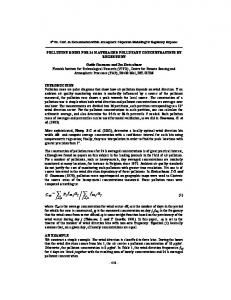
abuse (reported and substantiated) in the 90 days after program discharge. However, seven children did experience our “terminal” event (Column E), and thus were removed from the risk set at the next interval (i.e., 90-180 days). These basic counts of individual cases experiencing the event at a particular point in time are the basic ingredients for calculating survival and hazard rates, which both appear in Columns G and J, respectively. Survival Function The life table in Table 2 also shows the cumulative proportion of cases “surviving” at the end of each interval (Column H). This cumulative proportion always begins at one, since 100 percent of the sample will not have experienced the event on day one, and tapers off as individual cases drop out of the risk set (Singer & Willett, 1991). The cumulative survival rate expresses the likelihood of “surviving” a particular time interval. It is expressed as the probability of a case not experiencing the event over the study period (Singer & Willett, 1991). In our case, it is the likelihood of a child not experiencing an incident of child abuse after the family has been discharged from the family preservation program. As time passes and more cases experience the event, the survivor probability tapers off, and if the entire sample should experience the event before the end of the evaluation period, it would reach zero (Blossfield, Hamerle, & Mayer, 1991). The survival function is a useful diagnostic tool since it shows both the trend of an event happening over time and also the time point at which the event was most likely to occur. By graphing the cumulative survival rate (see Figure 1), we can observe the survival curve, which provides a visual of the overall “if and when” risk of child abuse to children after discharge from the family preservation program. At each point where the line becomes jagged and then drops (see Figure 1), an abuse incident occurred. We see in Figure 1 that while the risk of a child abuse incident is small the risk is never eliminated. The line makes its first drop at day 17 when the first incident of abuse occurred, and continues to step down on subsequent days when a case was reported to have experienced an abuse incident. Figure 1 is also useful for illustrating how much time has passed, on average, before half the sample has experienced the event (i.e., the survivor function reaches .50). In our example, the median survival time (i.e., time at which half the cases would experience a child abuse event after discharge from the FP program) was estimated at 1260 days (3.5) years. The survival curve clearly shows that while the risk for abuse after discharge from the Family Preserva-
56
ADMINISTRATION IN SOCIAL WORK FIGURE 1. Cumulative Survival Rate of Time to First Report of Abuse 1.1
Cumulative Survival Rate
1.0
.9
.8
.7 .6 −200
0
200
400
600
800
1000 1200
1400
Time in Days to First Report of Abuse
tion program is a small one, it is a risk that persists over time (up to 3 1/2 years for the program in our case example). Hazard Function The survival and hazard functions are inversely related, thus offering different views of the same problem. As mentioned earlier, the hazard function in our example is the probability that a case will experience an abuse incident in a specified time interval given that the abuse event had not yet been experienced by that case (Katz & Hauck, 1993). As the cumulative survival function drops to zero, the cumulative hazard function rises toward one to reflect a growing number of “failures” as more cases are reported for abuse over time (Singer & Willett, 1991). The hazard rate shown in the life table (see Column J in Table 2) gives the conditional probability of the abuse occurring in a given time interval (non-cumulative). The probability is conditional upon the number of cases that remain in the risk set at the beginning of an interval. Of interest to the program administrator is the level of risk for child abuse after discharge. Although the hazard rate shown in Table 2 is quite small, it does fluctuate over time. Figure 2 graphs the hazard rate over time and reveals that children are at greatest risk (7 in 10,000) for abuse in the 90 days immediately following program discharge, and then again almost three years after the program (6 in 10,000).
Yvonne A. Unrau and Heather Coleman
57
FIGURE 2. Daily Hazard Rate of Time to First Report of Abuse .0008
Hazard Rate
.0006
.0004
.0002
0.000 −0.002 −200
0
200
400
600
800 1000 1200 1400
Time in Days to First Report of Abuse
Thus, the hazard function can serve as a useful diagnostic tool for deciding program services such as the optimal length of follow-up services and the best time to give booster visits to families. Interpretation of the hazard function can uncover trends in the occurrence of the event, such as an increase or decrease in the hazard rate, times of peak rates, and how risk to sub-groups of clients compare. Stratification So far we have used tools of EHA to gain a better understanding of our dependent variable, or hazard rate, which is an estimate of both the occurrence and timing of an abuse incident after program discharge. Consequently, the survival and hazard functions examined in Figures 1 and 2 are considered baseline conditions; that is, they did not account for any of our three predictor variables (see Table 1), which might be associated with our hazard rate. Stratification is an option in EHA that provides a useful tool for examining risk of an event for subgroups of cases. With our three predictor variables, it is possible to divide our sample of 108 according to family size (e.g., small vs. large), family income under poverty level vs. over poverty level, and learning disability of children (e.g., yes vs. no). Figure 3 illustrates the cumulative survival curve for two subgroups of our sample that were defined by children with and without a learning disability.
58
ADMINISTRATION IN SOCIAL WORK
This stratified survival curve clearly shows that children with learning disabilities drop out of the “risk set” at a faster rate than children without learning disabilities. In other words, they were more likely to experience an incident of child abuse sooner in the post-discharge (or follow-up) period. Before drawing firm conclusions about the differential rate of risk for children with and without disabilities, it is important to establish whether or not the observed difference between groups in Figure 3 is “different” enough from our baseline observation to be of value for program decision-making. We want to know if our estimates that account for our predictor variables are significantly different from our baseline estimates (no predictors). Thus, we move on to yet another EHA tool–Cox Regression–to determine whether the added information of our predictor variable produces better estimates. Cox Regression Cox regression, as a tool in EHA, involves more statistics than any of the other tools discussed thus far. It is the most popular of the many different EHA techniques (Allison, 1984) and available in most statistical software packages. The appeal of Cox regression is that it can reveal relationships between char-
FIGURE 3. Cumulative Survival Curves for Children With and Without Learning Disabilities 1.1
Cumulative Survival
1.0 .9 .8 .7 .6 .5
Learning Disability
.4 .3 −200
Yes No 0
200
400
600 800 1000 1200 1400
Time in Days to First Report of Abuse
Yvonne A. Unrau and Heather Coleman
59
acteristics of clients and services and the probability of an outcome occurring. It can also identify whether particular client and service characteristics, or variables, contribute to elevated risk of abuse over time. The advantage of Cox regression as a statistical tool is that it brings more precision to the analysis and because statistics are used as the primary diagnostic tool (versus graphical representations), conclusions are more definitive. There are three major assumptions to consider prior to performing a Cox regression. The first two assumptions have already been discussed. First, the event must be defined in mutually exclusive terms; that is, at every point of interest, each individual can fall into only one state, meaning that at any point an individual has experienced the event or has not. Definite dates of abuse ensured that children were in one category only. Second, censored cases must have the quality of randomness (no patterns) so that we may have confidence that censored cases are independent, or unrelated to, the survival distribution (Greenhouse, Stangl, & Bromberg, 1989; Lachin & Foulkes, 1986; Katz & Hauck, 1993). The third assumption is “proportionality,” and is a consideration only when predictor variables are included in the analysis. Proportionality assumes that hazard rates for different values of a predictor variable (e.g., 0 = child has no learning disability, 1 = child has learning disability) remain constant over the observation period (Blossfeld, Hamerle, & Mayer, 1991). The tool of stratification plays an important role in assessing the proportionality assumption. Dividing the sample into strata according to the categorical values of a predictor variable (e.g., subgroups) will show whether that variable interacts with time, which is a situation to be avoided (Allison, 1984). In other words, the expectation is that the ratio of the hazards for each subgroup is constant over time. The assumption of proportionality can be tested by using procedures in SPSS such as the Log Minus Log test of proportionality. However, the basic idea can be understood by comparing survivor functions for different subgroups. At the very least, the two survival curves should never intersect as was the case in Figure 3. As it turns out, it is reasonable to expect that hazard ratios will not be constant over time and hence fail to fulfill the proportionality assumption (Schemper, 1992). The two major consequences of failing the assumption in a Cox regression is that the power of the analysis is decreased and the relative risk for predictors with hazard ratios that increase over time is overestimated while for predictors that are not proportional, the relative risk is often underestimated. Checking the proportionality assumption is an essential step in performing a Cox regression to assess the degree of bias that may be present in the results. While violation of the proportional hazards assumption may be the rule rather than the exception and the proportional hazards assumption is mythical in any
60
ADMINISTRATION IN SOCIAL WORK
set of data until otherwise proven (Singer & Willett, 1991), it is still necessary to check the assumption and report on it. Cox regression is based on the fundamental premises of the life table (Allison, 1984). Other than testing for proportionality, it makes no assumptions about the true shape of the distribution of the event and estimates the influence of covariates on the risk of the event occurring (Griffin, 1993; Singer & Willett, 1991). When building models that estimate the risk, the dependent variable in Cox regression is the hazard rate, which is the combined effect of all predictor variables on the survival time. It is semi-parametric because it recognizes the order in which events (dependent variables) occur, as well as the timing of events. It is parametric such that it specifies a regression model with a specific functional form; it is nonparametric insofar as it does not specify the exact timing of the event times (Allison, 1984, p. 14). Thus, Cox regression relies on the order of events (Griffin, 1993). It can therefore be used to assess the effects of predictors regardless of the pattern of event occurrence. Assessing Which Predictor Variables Get Entered into the Regression To determine which of our three predictor variables (see Table 1) to include into our regression analysis, we assess the association of each one with the dependent variable, or the hazard rate. This is accomplished by performing a separate Cox regression for each predictor variable and the hazard rate. The predictor variables that show significance at the bivariate analysis will then be entered into the multivariate analysis. Table 3 shows the regression output for three separate Cox regression analyses, one for each of the three predictor variables in our example. Table 3 shows that the output of EHA Cox regression is much the same as logistic regression. Indeed, the interpretation of the output is very similar. Beta TABLE 3. Bivariate Cox Regression Results B
SE
Wald
df
Sig.
Exp(B)
Family Income
⫺.599
.169
12.550
1
.000
.549
B
SE
Wald
df
Sig.
Exp(B)
Learning Disability
1.302
.500
6.789
1
.009
3.677
SE
Wald
df
Sig.
Exp(B)
.070
4.553
1
.033
1.162
B Family Size
.150
Yvonne A. Unrau and Heather Coleman
61
coefficient () measures the association between the predictor and the rate of the event, which in our case is an incident of child abuse. They are assessed to have a significant relationship with the hazard rate when the Wald Statistic shows a p-value (significance) that reaches the desired levels, which are typically set at .01 or .05. When  is statistically significant, it is useful to examine the exp(B) value in the output (see Table 3) as it provides a standardized estimate of the population parameters that can be interpreted as a type of relative risk. Beta Coefficients and their associated exp(B) assume the value “1” when the predictor variable has no effect upon the hazard rate. Values smaller than 1 indicate that the predictor variable has a negative influence on the hazard rate, and values greater than 1 indicate a positive relationship. Table 3 shows each of our three predictor variables as having an independent relationship with the hazard rate. In other words, all are related to the likelihood of a child abuse incident after discharge from the family preservation program. Family size and learning disability show a positive relationship, suggesting that both variables independently increase the hazard and therefore exert a negative impact on the length of survival. Thus, larger family size and the presence of a child with a learning disability both lessen the time it takes for a substantiated incident of abuse to occur. As the value of the covariate increases, the hazard also increases. Family income, on the other hand, has a negative coefficient, indicating that as income increases in value, the hazard decreases because it exerts a positive impact on the length of survival. With a few calculations, the exp(B) values provide added information such as the risk that each predictor variable poses. This is accomplished with the following equation: 100(Exp–1). Using family size as an example, 100 (1.162–1) equals 16.2%. This means that for every additional family member in a particular family, the risk of receiving a substantiated report of abuse increases 16.2%. The same calculation applied to the learning disability variable, which has an exp(B) > 1, produces the following result: 100(3.677–1) equals 267.7%, which means that children with learning disabilities have 267.7% greater chance of a child abuse incident compared to children without learning disabilities. We could also say that children with learning disabilities are 2.7 times more likely to experience an incident of child abuse. Diagnosing Cox Regression Output The advantage of Cox regression is in its ability to examine multiple predictor variables in a single analysis. Because we established that all three of our predictor variables are independently associated with the hazard rate, we enter all of them into the regression model in order to assess the combined effect of family size, family income, and learning disability on the risk of abuse.
62
ADMINISTRATION IN SOCIAL WORK
Forward stepwise regression was used because the study was exploratory and not based on any theoretical model. Table 4 shows the SPSS Cox regression output of the stepwise model at Steps 1, 2, and 3. Because the final model (Step 3) is additive, we can examine the impact of each of the three variables combined on the hazard rate. Employing the formula provided above, we can calculate: Hazard function = 100(3.677[learning disability] ⫺1) + 100(1.156[family size] ⫺1) + 100(.537[income] ⫺1). Therefore, a family with a learning disabled child, two family members (single parent and one child) and an income of less than $5,000 per year has a 3.5 times (352%) greater risk of an abuse incident as compared to a two-person family that earns the same income but does not have a learning disabled child. The results of this analysis combined with practice knowledge of working with at-risk families needing family preservation services, may suggest that three predictor variables are proxy measures of family stress that may contribute to abuse. These empirical findings can be used as one piece of information to assist workers in planning interventions to target stress management in families in an effort to further reduce the risk of future abuse incidents. CONCLUSION AND IMPLICATIONS EHA as a diagnostic tool can generate empirical information that can add to program planning efforts in several ways. One way that the results of EHA anal-
TABLE 4. Variables in the Equation at Steps 1, 2, and 3 B
SE
Wald
df
Sig.
Exp(B)
Step 1
Family Income
2.599
.169
12.550
1
.000
.549
Step 2
Learning Disability
1.346
.502
7.195
1
.007
3.614
Family Income
2.609
.171
12.634
1
.000
.544
Learning Disability
1.285
.502
6.544
1
.011
3.614
.145
.072
4.080
1
.043
1.156
2.621
.172
13.096
1
.000
.537
Step 3
Family Size Family Income
At Step 3: 22 Log likelihood beginning 224.05 22 Log likelihood end 201.735
Yvonne A. Unrau and Heather Coleman
63
ysis can be used is to assess their fit with practitioners’ expectations of client outcomes. For example, is there congruence between the beliefs of the FP practitioner and the finding that a child with learning disabilities increased the risk of abuse after program exit? This empirical finding may serve to validate the practice wisdom of workers in the program or create awareness of a key family characteristic that may have been previously overlooked. Checking out practitioners’ assumptions in this way can strengthen practitioners’ understanding and commitment to a program’s service delivery model. When EHA results and practitioner viewpoints agree, the empirical analysis may validate what practitioners already know, thereby giving welcomed recognition to their expertise. However, when EHA results and practitioner opinion disagree, it provides an opportunity either to consider additional variables in the EHA model (i.e., variables that practitioners believe may better explain the event) or the beginning of professional development that may involve a shift in practice thinking. Second, the results of EHA can aid decision-makers in making changes to a model of service delivery. For instance, the results of our FP example showed that the risk of child abuse is greatest within 90 days of exiting the program and then again three years after discharge. This finding would have great value in deciding whether or not the program should have a follow-up component, or how the follow-up should be configured. For example, if the FP program were structured to provide follow-up calls to families six months after discharge, a decision might be made to make such calls at least three months sooner. In the absence of other compelling information, EHA may be used to guide a course of action. Of course, the effect of the change in timing of follow-up calls could then be tested in future EHA analyses. Our analysis demonstrated the impact of three client characteristics on the probability of abuse occurring after service closure. We need to point out that, had we used service variables in the analysis, EHA could help identify service characteristics that either decrease or increase the probability of abuse recurring during follow-up. For example, Coleman (1995) found that individual counseling decreased the risk of abuse by 46.38% and family counseling decreased the risk of abuse by 40.94%. These findings offer direction to FP workers and administrators about what services might be provided to decrease the risk of abuse in the future. While EHA can be used to supplement professional or program development, it is only one tool. The statistical information that EHA produces is only as good as the data that it is based on, and as we have discussed in this article, EHA as a diagnostic tool is not without limitations. However, EHA used consistently over time can help social service administrators and decision-makers to build stronger service delivery models and fortify program evaluation efforts.
64
ADMINISTRATION IN SOCIAL WORK
NOTE 1. Left-censoring occurs when a case experiences the event at an unknown time before the evaluation or observation period even begins or when the start time is unknown. Ignoring left-censored cases creates bias by inflating risk estimates produced in EHA but since methods of analyzing left-censored data are not well-developed (Singer & Willett, 1991), we do not discuss them in this paper.
REFERENCES Allison, P. (1984). Event History Analysis: Regression for longitudinal event data. Sage University Paper series on quantitative applications in the Social Sciences, 07-046. Beverly Hills and London: Sage Publications. Barton, T., & Pillai, V. (1995). Using an event history analysis to evaluate social welfare programs. Research on Social Work Practice, 5(2), 176-192. Blossfeld, H., Hamerle, A., & Mayer, K. (1991). Event-history models in social mobility research. In D. Magnusson, L. Bergman, G. Rudinger, & B. Torestad (Eds.), Problems and methods in longitudinal research: Stability and change (pp. 212-225). Cambridge: Cambridge University Press. Burton, R., Johnson, R., & Clayton, R. (1996). The effects of role socialization on the initiation of cocaine use: An event history analysis from adolescence into middle adulthood. Health and Social Behavior, 37(1), 75-90. Coleman, H. (1995). A longitudinal study of a family preservation program. Unpublished doctoral dissertation, School of Social Work, University of Utah. Dickter, D., Roznowksi, M., & Harrison, D. (1996). Temporal tempering: An Event History Analysis of the process of voluntary turnover. Journal of Applied Psychology, 81(6), 705-716. Fahrmeir, L., & Klinger, A. (1998). A nonparametric multiplicative hazard model for event history analysis. Biometrika, 85(3), 581-592. Ford, I., Norrie, J., & Ahmadi, S. (1995). Model inconsistency, illustrated by the Cox proportional hazards model. Statistics in Medicine, 14(8), 735-746. Fraser, M., Pecora, P., Popuang, C., & Haapala, D. (1992). Event History Analysis: A Proportional Hazards perspective on modeling outcomes in Intensive Family Preservation Services. Journal of Social Service Research, 16(1/2), 123-158. Freedman, D., Thornton, A., Camburn, D., Alwin, D., & Young-DeMarco, L. (1988). The life history calendar: A technique for collecting retrospective data. Sociological Methodology, 18, Clifford Clogg, (Ed.) (pp. 37-68). Washington: American Sociological Association. Greenhouse, J., Stangl, D., & Bromberg, J. (1989). An introduction to survival analysis: Statistical methods for analysis of clinical trial data. Journal of Consulting & Clinical Psychology, 57(4), 536-544. Griffin, W. (1993). Event history analysis of marital and family interaction: A practical introduction. Journal of Family Psychotherapy, 6(3), 211-229. Heinzl, H., & Kaider, A. (1997). Gaining more flexibility in Cox proportional hazards regression models with cubic spline functions. Computer Methods and Programs in Biomedicine, 54(3), 201-208.
Yvonne A. Unrau and Heather Coleman
65
Hser, Y., Yamaguchi, K., Chen, J., & Anglin, M. (1995). Effects of interventions on relapse to narcotic addiction. Evaluation Review, 19(2), 123-140. Hutchison, D. (1988). Event history and survival analysis in the social sciences: Advanced applications and recent developments. Quality and Quantity, 22, 255-278. Katz, M., & Hauck, W. (1993). Proportional Hazards (Cox) Regression. Journal of General Internal Medicine, 8(12), 702-711. Kirk, R. S. (2004). Intensive family preservation services: Demonstrating placement prevention using event history analysis. Social Work Research, 28(1), 5-16. Lachin, J. (1981). Introduction to sample size determination and power analysis for clinical trials. Controlled Clinical Trials, 2, 93-113. Lachin, J., & Foulkes, M. (1986). Evaluation of sample size and power for analyses of survival with allowance for nonuniform patient entry, losses to follow-up, noncompliance, and stratification. Biometrics, 42, 506-519. Lachin, J., & Foulkes, M. (1986). Evaluation of sample size and power for analyses of survival with allowance for nonuniform patient entry, losses to follow-up, noncompliance and stratification. Biometrics, 42, 507-519. Nugent, W., Sieppert, J., & Hudson, W. (2001). Practice evaluation for the 21st Century. Belmont, CA: Wadsworth/Thomson Learning. Rank, M. R. (1985). Exiting from welfare: A life-table analysis. Social Service Review, 59, 358-376 Schemper, M. (1992). Cox analysis of survival data with non-proportional hazard functions. The Statistician, 41, 455-465. Singer, J., & Willett, J. (1991). Modeling the days of our lives: Using survival analysis when designing and analyzing longitudinal studies of duration and timing of events. Psychological Bulletin, 110(2), 268-290. Smith, K., Zick, C., & Duncan, G. (1991). Remarriage patterns among recent widows and widowers. Demography, 28(3), 361-374. Sytema, S., Micciolo, R., & Tansella, M. (1996). Service utilization by schizophrenic patients in Groningen and South-Verona: An event history analysis. Psychological Medicine, 26(1), 109-119. Tabachnick, B., & Fidell, L. (2001). Using multivariate statistics. Boston: Allyn & Bacon. Yamaguchi, K. (1991). Event History Analysis. Newbury Park, CA: Sage.