functions) are defined differently. This paper describes a theory for reconciling the two approaches. I introduce a pair of asymptotic pseudounitary operators, ...
GEOPHYSICS, VOL. 68, NO. 3 (MAY-JUNE 2003); P. 1032–1042, 6 FIGS. 10.1190/1.1581074
Asymptotic pseudounitary stacking operators
Sergey Fomel∗ An integral operator often is used to represent the forward modeling problem, and we invert it to solve for the model. In this paper, I consider two different approaches to inversion. The first is least-squares inversion, which requires constructing the adjoint counterpart of the modeling operator. The second approach is asymptotic inversion, which aims at reconstructing the high-frequency (discontinuous) parts of the model. I compare the two approaches and introduce the notion of asymptotic pseudounitary operator pair that ties them together. In practice, least-squares inversion is often applied as an iterative process (Ronen and Liner, 2000). The advantage of connecting it with the asymptotic inverse theory is the ability to speed up the iteration. This approach was used, in the context of seismic migration, by Jin et al. (1992) and Lambare´ et al. (1992). Asymptotic pseudounitary operators, introduced in this paper, provide a more universal theoretical tool. One can use them to construct an appropriate preconditioning operator for accelerating the convergence of the least-squares methods. The first part of this paper contains a formal definition of a stacking operator and reviews the theory of asymptotic inversion, following the fundamental results of Beylkin (1985) and Goldin (1988, 1990). According to this theory, the highfrequency asymptotic inverse of a stacking operator is also a stacking operator. To connect this theory with the theory of adjoint operators, I show that the adjoint of a stacking operator can also be included in the class of stacking operators. The adjoint operator has the same summation path as the asymptotic inverse but a different weighting function. These two results combine together to form the definition of asymptotic pseudounitary integral operators. I apply such operators to define a general preconditioning operator for least-squares inversion. Although one can apply Beylkin’s theory directly for constructing an appropriate asymptotic preconditioner, pseudounitary operators accomplish this job in a more straightforward and computationally attractive way. The second part of the paper addresses such examples of commonly used stacking operators as wave-equation datuming, migration, velocity transform, and offset continuation. The theory is specified for these particular applications and
ABSTRACT
Stacking operators are widely used in seismic imaging and seismic data processing. Examples include Kirchhoff datuming, migration, offset continuation, dip moveout, and velocity transform. Two primary approaches exist for inverting such operators. The first approach is iterative least-squares optimization, which involves the construction of the adjoint operator. The second approach is asymptotic inversion, where an approximate inverse operator is constructed in the high-frequency asymptotics. Adjoint and asymptotic inverse operators share the same kinematic properties, but their amplitudes (weighting functions) are defined differently. This paper describes a theory for reconciling the two approaches. I introduce a pair of asymptotic pseudounitary operators, which possess both the property of being adjoint and the property of being asymptotically inverse. The weighting function of the asymptotic pseudounitary stacking operators is shown to be completely defined by the derivatives of the operator kinematics. I exemplify the general theory by considering several particular examples of stacking operators. Simple numerical experiments demonstrate a noticeable gain in efficiency when the asymptotic pseudounitary operators are applied for preconditioning iterative least-squares optimization.
INTRODUCTION
Integral (stacking) operators play an important role in seismic imaging and seismic data processing. The most common applications are common midpoint stacking, Kirchhoff migration, and dip moveout. Other examples include (listed in random order) Kirchhoff datuming, back-projection tomography, slant stack, velocity transform, offset continuation, and azimuth moveout. The use of the integral methods increases in prestack three-dimensional processing because of their flexibility with respect to irregularities in the data geometry.
Published on Geophysics Online December 19, 2002. Manuscript received by the Editor November 20, 2000; revised manuscript received November 4, 2002. ∗ University of Texas at Austin, Bureau of Economic Geology, University Station, Box X, Austin, Texas 78713-8972. E-mail: sergey.fomel@ beg.utexas.edu. ° c 2003 Society of Exploration Geophysicists. All rights reserved. 1032
Asymptotic Pseudounitary Operators
accompanied by numerical examples. The examples demonstrate the practical advantages of asymptotic pseudounitary operators. THEORETICAL DEFINITION OF A STACKING OPERATOR
In practice, integration of discrete data is performed by stacking. In theory, it is convenient to represent a stacking operator in the form of a continuous integral:
Z
S(t, y) = A[M(z, x)] =
Ä
w(x; t, y)M(θ (x; t, y), x)d x. (1)
Function M(z, x) is the input of the operator, S(t, y) is the output, Ä is the summation aperture, θ represents the summation path, and w stands for the weighting function. The range of integration (the operator aperture) may also depend on t and y. Allowing x to be a two-dimensional variable, we can use definition (1) to represent an operator applied to three-dimensional data. Throughout this paper, I assume that t and z belong to a one-dimensional space, and that x and y have the same number of dimensions. ˆ The goal of inversion is to reconstruct some function M(z, x) ˆ is in some sense close to M in for a given S(t, y), so that M equation (1). ASYMPTOTIC INVERSION: RECONSTRUCTING THE DISCONTINUITIES
Mathematical analysis of the inverse problem for operator (1) shows that only in rare cases can we obtain an analytically exact inversion. A well-known example is the Radon transform, which has acquired a lot of different aliases in geophysical literature: slant stack, tau-p transform, plane wave decomposition, and controlled directional reception (CDR) transform (Gardner and Lu, 1991). In this case,
θ(x; t, y) = t + x y,
(2)
w(x; t, y) = 1.
(3)
Radon obtained a result similar to the theoretical inversion of operator (1) with the summation path (2) and the weighting function (3) in 1917, but his result was not widely known until the development of computer tomography. According to Radon (1917), the inverse operator has the form
Z
−1
M(z, x) = A [S(t, y)] = |D|
ˆ wS( ˆ θ(y; z, x), y)dy,
m
(4) where
ˆ θ(y; z, x) = z − x y,
(5)
1 , (2π)m
(6)
wˆ =
|D| is a one-dimensional convolution operator with the spectrum |ω|:
1 |D|[U (z, x)] = 2π
Z
Z
U (ξ, x)
|ω|e
iω(z−ξ )
dωdξ,
(7)
and m is the dimensionality of x and y (usually 1 or 2). In Russian geophysical literature, a similar result for the inversion of the CDR transform was published by Nakhamkin (1969).
1033
Extension of Radon’s result to the general form of integral operator (1) (generalized Radon transform) is possible via asymptotic analysis of the inverse problem. In the general case, Beylkin (1985) and Goldin (1988) have shown that asymptotic inversion can reconstruct discontinuous parts of the model. These are the parts responsible for the asymptotic behavior of the model at high frequencies. Since the discontinuities are associated with wavefronts and reflection events on seismic sections, there is a certain correspondence between asymptotic inversion and such standard goals of seismic data processing as kinematic equivalence and amplitude preservation. The main theorem of asymptotic inversion can be formulated as follows (Goldin, 1988). The leading-order discontinuities in M are reconstructed by an integral operator of the form
ˆ ˆ M(z, x) = A[S(t, y)] Z = |D|m w(y; ˆ z, x)S(θˆ (y; z, x), y)dy,
(8)
where the summation path θˆ is obtained simply by solving the equation
z = θ (x; t, y)
(9)
for t (if such an explicit solution is possible). The correctly chosen summation path reconstructs the geometry of the discontinuities. To recover the amplitude, we must choose the correct weighting function, which is constrained by the equation (Beylkin, 1985; Goldin, 1988)
s
1 wwˆ = (2π )m
¯ ¯m ¯ ∂ θˆ ¯ ˆ |F F|¯¯ ¯¯ , ∂z
(10)
where
F=
∂θ ∂ 2 θ ∂θ ∂ 2 θ − , ∂t ∂ x∂ y ∂ y ∂ x∂t
(11)
Fˆ =
∂ θˆ ∂ 2 θˆ ∂ θˆ ∂ 2 θˆ − . ∂z ∂ x∂ y ∂ x ∂ y∂z
(12)
The solution assumes that differential forms F and Fˆ exist and are bounded and non-vanishing. [This requirement is related to the requirement for the normal AT A operator, inroduced in the next section, to be a pseudodifferential operator (Wong, 1991). Situations where this condition is violated require a special consideration (Nolan and Symes, 1996; Stolk, 2000).] In the multidimensional case (m ≥ 2), they are replaced by the determinants of the corresponding matrices. To ensure the asymptotic inversion, equation (10) must be satisfied at least in the vicinity of the stationary points of integral (1). Those are the points where the summation path of the form (9) is tangent to the traveltimes of the actual events on the transformed model. ˆ = |∂ θˆ /∂z| = 1, and In the case of the Radon transform, |F F| the asymptotic inverse coincides with the exact inversion. LEAST-SQUARES INVERSION AND ADJOINT OPERATORS
Least-squares inversion is widely used in practice not only because it is applicable even when the asymptotic results are unavailable but also because of its ability to handle finite sampling effects that are difficult to handle in asymptotic theory (Ronen and Liner, 2000).
1034
Fomel
The theoretical least-squares inverse of operator (1) has the well-known form (Tarantola, 1987)
˜ ˜ M(z, x) = A[S(t, y)] = (AT A)† AT [S(t, y)],
(13)
where † denotes pseudo-inverse, and the adjoint operator A is defined by the dot-product test:
(S(t, y), A[M(z, x)]) ≡ (AT [S(t, y)], M(z, x)).
(14)
(15)
In the case of integral operators, a natural definition of the dot-product is the double integral
ZZ
(S1 (t, y), S2 (t, y)) =
S1 (t, y)S2 (t, y)dydt,
(16)
ZZ (M1 (z, x), M2 (z, x)) =
M1 (z, x)M2 (z, x)d xdz. (17)
The notion of the adjoint operator completely depends on the arbitrarily chosen definition of the dot product and norm in the model and data spaces. A simple way to change those definitions is to find some positive weights W M (z, x) in the model space and W S (t, y) in the data space that define the dot products as follows:
(S1 (t, y), S2 (t, y)) ZZ = W S (t, y)S1 (t, y)S2 (t, y)dydt,
(18)
(M1 (z, x), M2 (z, x)) ZZ = W M (z, x)M1 (z, x)M2 (z, x)d xdz.
(19)
To formally define the adjoint of a stacking operator, let us substitute the definition of the stacking operator (1) into the dot product (14), as follows:
ZZZ
(S(t, y), A[M(z, x)]) =
w(x; t, y) × M(θ(x; t, y), x)S(t, y)d xd ydt. (20)
Assuming that the function θ is monotonic in t [if this is not the case, a different parameterization of the stacking function is appropriate (Fomel, 2001)], we can change the integration variable t to z = θ(x; t, y) and rewrite equation (20) in the form
ZZZ
(S(t, y), A[M(z, x)]) =
Z AT [S(t, y)] =
w(y; ˜ z, x)S(θˆ (y; z, x), y)dy.
Thus we have proven that the continuous adjoint of a stacking operator is another stacking operator. The adjoint operator has the same summation path as the asymptotic inverse (8), which guarantees the correct reconstruction of the kinematics of the input wavefield. The amplitude (weighting function) of the adjoint operator is directly proportional to the forward weighting according to equation (22). The coefficient of proportionality is the Jacobian of the transformation of the variables z and t. Similar results have been obtained for particular cases of stacking operators: velocity transform (Thorson, 1984; Jedlicka, 1989), Kirchhoff constant-velocity migration (Ji, 1994), and normal moveout (Crawley, 1995). In the Appendix, I give an example of an application of least-squares inversion by reviewing inversion of the Radon operator and showing that it is precisely equivalent to the asymptotic result of the previous section. ASYMPTOTIC PSEUDOUNITARY OPERATOR PAIR
According to the theory of asymptotic inversion, briefly reviewed in the first part of this paper, the weighting function of the asymptotic inverse operator is inversely proportional to the weighting of the forward operator. On the other hand, the weighting in the adjoint is directly proportional to the forward weighting. This difference allows us to define a hybrid pair of operators that possess both the property of being adjoint and the property of being asymptotic inverses. It is appropriate to call a pair of operators defined in this way asymptotic pseudounitary. The definition of asymptotic pseudounitary operators follows directly from the combination of definitions (8) and (23). Splitting the derivative operator |D| in definition (8) into the product of two operators, we can write the forward operator as
S(t, y) = A[M(z, x)] Z = w(+) (x; t, y)|D|m/2 M(θ (x; t, y), x)d x
ˆ × S(θ(y; z, x), x)d yd xdz, (21) where θˆ has the same meaning as in equation (8), and
˜ ˜ M(z, x) = A[S(t, y)] Z = |D|m/2 w(−) (y; z, x)S(θˆ (y; z, x), y)dy. (25) According to equation (10),
w
(+)
w
(−)
w
s
1 = (2π )m
According to equation (22),
(22)
(24)
and its asymptotic pseudounitary adjoint as
w(y; ˜ z, x)M(z, x)
¯ ¯ ¯ ∂ θˆ ¯ ˆ w(y; ˜ z, x) = w(x; θ(y; z, x), y)¯¯ ¯¯. ∂z
(23)
T
With a specified definition of the dot-product, the generalized inverse minimizes the following quantity, which is the squared L 2 norm of the residual:
(S(t, y) − A[M(z, x)], S(t, y) − A[M(z, x)]).
Comparing equations (21) and (14), we conclude that the adjoint operator AT is defined by the equality
(−)
=w
¯ ¯m ¯ ∂ θˆ ¯ ˆ ¯ ¯ . |F F| ¯ ∂z ¯
¯ ¯ ¯ ˆ¯ ¯ ¯ ∂z ¯.
(+) ¯ ∂ θ
(26)
(27)
Asymptotic Pseudounitary Operators
Combining equations (26) and (27) uniquely determines both weighting functions, as follows:
w
(+)
w(−)
¯ ¯(m−2)/4 ¯ ˆ¯ 1 1/4 ¯ ∂ θ ¯ ˆ = |F F| ¯ ¯ , m/2 (2π) ∂z ¯ ¯(m+2)/4 ¯ ∂ θˆ ¯ 1 1/4 ¯ ¯ ˆ = |F F| . ¯ ∂z ¯ m/2 (2π)
Equations (28) and (29) complete the definition of an asymptotic pseudounitary operator pair. The notion of pseudounitary operators is directly applicable in the situations where we can arbitrarily construct both forward and inverse operators. One example of such a situation is the velocity transform considered in the next section of this paper. In the more common case, the forward operator is strictly defined by the physics of a problem. In this case, we can include asymptotic inversion in the iterative least-squares inversion by means of preconditioning (Jin et al., 1992; Lambare´ et al., 1992). The linear preconditioning operator should transform the forward stacking-type operator to the form (24) with the weighting function (28). Theoretically, this form of preconditioning should lead to the fastest convergence of the iterative least-squares inversion with respect to the high-frequency parts of the estimated model. If the forward pseudounitary operator A p can be related to the forward modeling operator Am as A p = Ws Am Wm , where Ws and Wm are weighting operators in the data and model domains, respectively, then preconditioning simply amounts to replacing the least-squares equation
S ≈ Am [M]
Substituting the summation path formulas (32) and (33) into the general weighting function formulas (28) and (29), we immediately obtain
(28) (29)
(30)
w (+) = w(−) =
p ¯ ¯ cos α(x) cos α(y) ¯¯ ∂ 2 T ¯¯−1/2 R(x, y) = , ¯ ∂ x∂ y ¯ v(x)
EXAMPLES
In this section, I consider several particular examples of stacking operators used in seismic data processing and derive their asymptotic pseudounitary versions. Datuming Let x denote a point on the surface at which the propagating wavefield is recorded. Let y denote a point on another surface to which the wavefield is propagating. Then, the summation path of the stacking operator for the forward wavefield continuation is
θ(x; t, y) = t − T (x, y),
(32)
where t is the time recorded at the y-surface, and T (x, y) is the traveltime along the ray connecting x and y. The backward propagation reverses the sign in equation (32), as follows:
ˆ θ(y; z, x) = z + T (x, y).
(33)
(34)
(35)
where v(x) is the velocity at the point x, and α(x) and α(y) are the angles formed by the ray with the x and y surfaces, respectively. In a constant-velocity medium,
R(x, y) = v m−1 T (x, y)m/2 .
(36)
Gritsenko’s formula (35) allows us to rewrite equation (34) in the form (Goldin, 1988)
p cos α(x) cos α(y) , (37) w v(x)R(x, y) p 1 cos α(x) cos α(y) (−) w (y; z, x) = . (38) (2π )m/2 v(y)R(y, x) (+)
1 (x; t, y) = (2π )m/2
The weighting functions commonly used in Kirchhoff datuming (Berryhill, 1979; Wiggins, 1984; Goldin, 1985) are defined as
(31)
where P is the preconditioned model. The advantage of using equation (31) is in the the fact that the normal operator ATp A p is closer (asymptotically) to identity and therefore should be easier to invert than the original operator AmT Am in the leastsquares solution (13).
¯ ¯ 1 ¯¯ ∂ 2 T ¯¯1/2 . (2π )m/2 ¯ ∂ x∂ y ¯
Gritsenko’s formula (Gritsenko, 1984; Goldin, 1986) states that the second mixed traveltime derivative ∂ 2 T /∂ x∂ y is connected with the geometric spreading R along the x-y ray by the equality
with the equation
Ws [S] ≈ Ws Am Wm [P] = A p [P],
1035
w(x; t, y) =
1 cos α(x) , (2π )m/2 v(x)R(x, y)
(39)
w(y; ˆ z, x) =
cos α(y) 1 . m/2 (2π ) v(y)R(y, x)
(40)
These two operators appear to be asymptotically inverses according to formula (10). They coincide with the asymptotic pseudounitary operators if the velocity v is constant [v(x) = v(y)], and the two datum surfaces are parallel [α(x) = α(y)]. Migration Least-squares migration, envisioned by Lailly (1984) and Tarantola (1984), has recently become a practical method and gained a lot of attention in the geophysical literature (Chavent and Plessix, 1999; Duquet and Marfurt, 1999; Nemeth et al., 1999; Fomel et al., 2002). Using the theory of asymptotic pseudounitary operators allows us to reconcile this approach with the method of asymptotic true-amplitude migration (Bleistein et al., 2001). As recognized by Tygel et al. (1994), true-amplitude migration (Goldin, 1992; Schleicher et al., 1993) is the asymptotic inversion of seismic modeling represented by the Kirchhoff highfrequency approximation. The Kirchhoff approximation for a reflected wave (Haddon and Buchen, 1981; Bleistein, 1984) belongs to the class of stacking-type operators as defined by equation (1) with the summation path
θ (x; t, y) = t − T (s(y), x) − T (x, r (y)),
(41)
1036
Fomel
the weighting function
w(x; t, y) =
1 C(s(y), x, r (y)) , (2π)m/2 R(s(y), x)R(x, r (y))
(42)
and the additional time filter (∂/∂z)m/2 . Here x denotes a point at the reflector surface, s is the source location, and r is the receiver location at the observation surface. The parameter y corresponds to the configuration of observations. That is, s(y) = s, r (y) = y for the common-shot configuration, s(y) = r (y) = y for the zero-offset configuration, and s(y) = y − h, r (y) = y + h for the common-offset configuration (where h is the half-offset). The functions T and R have the same meaning as in the datuming example, representing the one-way traveltime and the oneway geometric spreading, respectively. The function C(s, x, r ) is known as the obliquity factor. Its definition is
µ ¶ 1 cos αs (x) cos αr (x) C(s, x, r ) = + , 2 vs (x) vr (x)
cos α(x) . v(x)
θˆ (y; z, x) = z + T (s(y), x) + T (x, r (y))
(44)
The stationary point of the Kirchhoff integral is the point where the stacking curve (41) is tangent to the actual reflection traveltime curve. When our goal is asymptotic inversion, it is appropriate to use equation (44) in place of equation (43) to construct the inverse operator. The weighted function (42) can include other factors affecting the leading-order (WKBJ) ray amplitude, such as the source signature, caustics counter (the KMAH index), and transmission coefficient for the interfaces ˇ (Chapman and Drummond, 1982; Cerven y, ˇ 2001). In the following analysis, I neglect these factors for simplicity. The model M implied by the Kirchhoff modeling integral is the wavefield with the wavelet shape of the incident wave and the amplitude proportional to the reflection coefficient from the reflector surface. The goal of true-amplitude migration is to recover M from the observed seismic data. In order to obtain the image of the reflectors, the reconstructed model is evaluated at the time z equal to zero. The Kirchhoff modeling integral requires explicit definition of the reflector surface. However, its inverse doesn’t require explicit specification of the reflector location. For each point of the subsurface, one can find the normal to the hypothetical reflector by bisecting the angle between the s − x and x − r rays. Born scattering approximation provides a different physical model for the reflected waves. According to this approximation, the recorded waves are viewed as scattered on smooth local inhomogeneities rather than reflected from sharp reflector surfaces. The inversion of Born modeling (Bleistein, 1987; Miller et al., 1987) closely corresponds with the result of Kirchhoff integral inversion. For an unknown reflector and the correct macrovelocity model, the asymptotic inversion reconstructs the signal located at the
(45)
to reconstruct the geometry of the reflector in the migrated section. According to equation (8), the asymptotic reconstruction of the wavelet requires, in addition, the derivative filter (−∂/∂t)m/2 . The asymptotic reconstruction of the amplitude defines the true-amplitude weighting function in accordance with equation (10), as follows:
w(y; ˆ z, x) =
(43)
where the angles αs (x) and αr (x) are formed by the incident and reflected waves with the normal to the reflector at the point x, and vs (x) and vr (x) are the corresponding velocities in the vicinity of this point. In this paper, I leave the case of converted (e.g., P-SV) waves outside the scope of consideration and assume that vs (x) equals vr (x) (e.g., P-P reflection). In this case, it is important to notice that at the stationary point of the Kirchhoff integral, αs (x) = αr (x) = α(x) (the law of reflection), and therefore
C(s, x, r ) =
reflecting surface with the amplitude proportional to the reflection coefficient. As follows from the form of the summation path (41), the integral migration operator must have the summation path
v(x)R(s(y), x)R(x, r (y)) (2π )m/2 cos α(x) ¯ ¯ 2 ¯ ∂ T (s(y), x) ∂ 2 T (x, r (y)) ¯ ¯. (46) ¯ + ׯ ¯ ∂ x∂ y ∂ x∂ y
The weighting function of the asymptotic pseudounitary migration is found analogously to equation (34) as
w
(+)
=w
(−)
¯ ¯ 1 ¯¯ ∂ 2 T (s(y), x) ∂ 2 T (x, r (y)) ¯¯1/2 = + ¯ . (2π )m/2 ¯ ∂ x∂ y ∂ x∂ y
(47) Unlike true-amplitude migration, this type of migration operator does not change the dimensionality of the input. Several specific cases exist for different configurations of the input data. Common-shot migration In the case of common-shot migration, we can simplify equation (46) with the help of Gritsenko’s formula (35) to the form
wˆ C S (r ; z, x) = =
1 cos α(r ) R(s, x) m/2 (2π ) v(x) R(x, r ) cos α(r ) R(s, x) 1 , (2π )m/2 v(r ) R(r, x)
(48)
where the angle α(r ) is measured between the reflected ray and the normal to the observation surface at the receiver point r . Formula (48) coincides with the analogous result of Keho and Beydoun (1988), derived directly from Claerbout’s imaging principle (Claerbout, 1970). An alternative derivation is given by Goldin (1987). Docherty (1991) points out a remarkable correspondence between this formula and the classic results of Born scattering inversion (Bleistein, 1987). For common-shot migration, pseudounitary weighting coincides with the weighting of datuming and corresponds to the downward continuation of the receivers. Zero-offset migration In the case of zero-offset migration, Gritsenko’s formula simplifies the true-amplitude migration weighting function (46) to the form
wˆ Z O (y; z, x) =
2m cos α(y) . (2π )m/2 v(y)
(49)
In a constant-velocity medium, one can accomplish true-amplitude zero-offset migration by premultiplying
Asymptotic Pseudounitary Operators
the recorded zero-offset seismic section by the factor (v/2)m−1 (t/2)m/2 [which corresponds at the stationary point to the geometric spreading R(x, y)] and downward continuation according to formula (40) with the effective velocity v/2 (Goldin, 1987; Hubral et al., 1991). This conclusion is in agreement with the analogous result of Born inversion (Bleistein et al., 1985), though derived from a different viewpoint. In the zero-offset case, the pseudounitary forward operator reduces to downward pseudounitary continuation with a velocity of v/2. Common-offset migration In the case of common-offset migration in a general variablevelocity medium, the weighting function (46) cannot be simplified to a different form, and all its components need to be ˇ calculated explicitly by dynamic ray tracing (Cerven yˇ and de Castro, 1993). In the constant-velocity case, we can differentiate the explicit expression for the summation path
θˆ (y; z, x) = z +
ρs (x, y) + ρr (x, y) , v
ρs (y, x) = ρr (y, x) =
q
2.5-D common-offset migration in a constant velocity medium (Sullivan and Cohen, 1987):
¡ ¢ √ x3 ρs + ρr ρs2 + ρr2 1 wˆ CO; 2.5D (y; z, x) = √ (2π )1/2 v(ρs ρr )3/2
The corresponding time filter for 2.5-D migration is (−∂/∂t)1/2 . In the common-offset case, the pseudounitary weighting is defined from equations (47) and (53) as follows: (−)
wC O (y; z, x) 1 = (2π v)m/2
x32 + (x1 − y1 − h 1 )2 + (x2 − y2 − h 2 )2 . (52)
For simplicity, the vertical component of the midpoint y3 is set here to zero. Evaluating the second derivative term in formula (46) for the common-offset geometry leads, after some heavy algebra, to the expression
µ cos α =
(x − y)2 + ρs ρr − h 2 2ρs ρr
+ ρr2
, (57)
¶1/2 .
(58)
An interesting example of a stacking operator is the hyperbola summation used for time migration in the poststack domain. In this case, the summation path is defined as
r
θˆ (y; z, x) =
(x − y)2 , v2
z2 +
(59)
where z denotes the vertical traveltime, x and y are the horizontal coordinates on the migrated and unmigrated sections, respectively, and v stands for the effectively constant root-meansquare velocity (Claerbout, 1995). The summation path for the inverse transformation (demigration) is found by solving equation (59) for z. It has the well-known elliptic form
r
t2 −
(x − y)2 . v2
(60)
The Jacobian of transforming z to t is
¯ ¯ ¯ ∂ θˆ ¯ z ¯ ¯= . ¯ ∂z ¯ t
(53)
¡ ¢ x3 (ρs + ρr )m−1 ρs2 + ρr2 1 wˆ C O (y; z, x) = . (54) (2π)m/2 v(ρs ρr )m/2+1
Equation (54) is similar to the result obtained by Sullivan and Cohen (1987). In the case of zero offset h = 0, it reduces to equation (49). Note that the value of m = 1 in equation (54) corresponds to the two-dimensional (cylindrical) waves recorded on the seismic line. A special case is the 2.5-D inversion, where the waves are assumed to be spherical while the recording is on a line, and the medium has cylindrical symmetry. In this case, the modeling weighting function (42) transforms to (Deregowski and Brown, 1983; Bleistein, 1986)
√ vC(s(y), x, r (y)) p , ρs ρr (ρs + ρr )
m−1 p 2 ρs2 m+1 (ρs ρr ) 2
x3 cos α(ρs + ρr )
θ (x; t, y) =
Substituting equation (53) into the general formula (46) yields the weighting function for the common-offset true-amplitude constant-velocity migration:
1 w(x; t, y) = (2π)1/2
√
where
x32 + (x1 − y1 + h 1 )2 + (x2 − y2 + h 2 )2 , (51)
¯ ¯ 2 ¯ ∂ T (s(y), x) ∂ 2 T (x, r (y)) ¯ ¯ ¯ + ¯ ¯ ∂ x∂ y ∂ x∂ y ¡ 2 ¢ µ ¶ x3 ρs + ρr2 ρs + ρr m−1 = cos α(x). v(ρs ρr )2 vρs ρr
(56)
Poststack time migration
(50)
where ρs and ρr are the lengths of the incident and reflected rays:
q
1037
(55)
and the time filter is (∂/∂z)1/2 . Combining this result with formula (53) for m = 1, we obtain the weighting function for the
(61)
If the migration weighting function is defined by conventional downward continuation (Schneider, 1978), it takes the following form, which is equivalent to equation (40):
w(y; ˆ z, x) =
1 1 cos α(y) cos α . (62) = (2π )m/2 v R(y, x) (2π )m/2 v m t m/2
The simple trigonometry of the reflected ray suggests that the cosine factor in formula (62) is equal to the simple ratio between the vertical traveltime z and the zero-offset reflected traveltime t:
z cos α = . t
(63)
The equivalence of the Jacobian (61) and the cosine factor (63) has important interpretations in the theory of Stolt frequencydomain migration (Stolt, 1978; Chun and Jacewitz, 1981; Levin, 1986). According to equation (22), the weighting function of the adjoint operator is the ratio of (62) and (61):
w(x; ˜ t, y) =
1 1 . m/2 m (2π ) v t m/2
(64)
1038
Fomel
We can see that the cosine factor z/t disappears from the adjoint weighting. This is completely analogous to the known effect of “dropping the Jacobian” in Stolt migration (Harlan, 1983; Levin, 1994). The product of the weighting functions for the time migration and its asymptotic inverse is defined according to formula (10) as
s
w wˆ =
1 (2π)m
¯ ¯m ¯ ∂ θˆ ¯ 1 ˆ |F F|¯¯ ¯¯ = 2 m . ∂z (v t)
(65)
Thus, the asymptotic inverse of the conventional time migration has the weighting function determined from equations (10) and (62) as
w(x; t, y) =
1 t/z . m/2 m (2π) v t m/2
(66)
The weighting functions of the asymptotic pseudounitary operators are obtained from formulas (28) and (29). They have
the form
√ 1 t/z . (2π )m/2 v m t m/2 √ 1 z/t w (−) (y; z, x) = . (2π )m/2 v m t m/2 w (+) (x; t, y) =
(67) (68)
The square roots of the cosine factor appearing in formulas (67) and (68) correspond to the analogous terms in the pseudounitary Stolt migration proposed by Harlan and Sword (1986). Figure 1 shows the output of a simple numerical test. The synthetic zero-offset section used in this test is shown in the left plot of Figure 2. The data are taken from Claerbout (1995) and correspond to a synthetic reflectivity model, which contains several dipping layers, a fault, and an unconformity. The input zero-offset section is inverted using an iterative conjugategradient method and two different weighting schemes: the uniform weighting and the asymptotic pseudounitary weighting [equations (67)–(68)]. I compare the iterative convergence by measuring the least-squares norm of the data residual error at different iterations. Figure 1 shows that the pseudounitary weighting provides a significantly faster convergence. The result of inversion after 10 conjugate-gradient iterations is shown in Figures 2 and 3. The right plot in Figure 2 shows the output of the least-squares migration. Figure 3 shows the corresponding modeled data and the residual error. The latter is very close to zero. Although this example has only a pedagogical value, it clearly demonstrates possible advantages of using asymptotic pseudounitary operators in least-squares migration. Velocity transform Velocity transform is another form of hyperbolic stacking with the summation path
θˆ (h; t0 , s) = FIG. 1. Comparison of convergence of the iterative least-squares migration. The dashed line corresponds to the unweighted (uniformly weighted) operator. The solid line corresponds to the asymptotic pseudounitary operator. The latter provides a noticeably faster convergence.
q t02 + s 2 h 2 ,
(69)
where h corresponds to the offset, s is the stacking slowness, and t0 is the estimated zero-offset traveltime. Hyperbolic stacking is routinely applied for scanning velocity analysis in common-midpoint stacking. Velocity transform inversion has proved to be a powerful tool for data interpolation and
FIG. 2. Input zero-offset section (left) and the corresponding least-squares image (right) after 10 iterations of iterative inversion.
Asymptotic Pseudounitary Operators
amplitude-preserving multiple suppression (Thorson, 1984; Ji, 1995; Lumley et al., 1995). Solving equation (69) for t0 , we find that the asymptotic inverse and adjoint operators have the elliptic summation path
θ(s; t, h) =
p t 2 − s2h2.
(70)
The weighting functions of the asymptotic pseudounitary velocity transform are found using formulas (28) and (29) to have the form
w (+) w (−)
√ √ ¯ ¯−1/4 ¯ ˆ¯ 1 1 sh t/t0 1/4 ¯ ∂ θ ¯ ˆ . (71) = |F F| ¯ ¯ =√ √ 1/2 (2π ) ∂t0 π t √ √ ¯ ¯3/4 ¯ ˆ¯ 1 1 sh t0 /t 1/4 ¯ ∂ θ ¯ ˆ . (72) = |F F| ¯ ¯ = √ √ 1/2 (2π ) ∂t0 π t
√ The factor sh for pseudounitary velocity transform weighting was discovered empirically by Claerbout (1995). Figure 4 shows the output of a numerical test of the leastsquares velocity transform inversion using a common midpoint (CMP) gather from the Mobil amplitude variation with offset (AVO) dataset (Lumley et al., 1995). The input CMP gather (shown in the left plot of Figure 5) is inverted using an iterative conjugate-gradient method and two different weighting scheme: the uniform weighting and the asymptotic pseudounitary weights [equations (71)–(72)]. Analogously to Figure 1, the iterative convergence is measured by the least-squares norm of the data residual error at different iterations. Figure 4 shows that the pseudounitary weighting provides a noticeably faster convergence in the first three iterations. At later iterations, the residual errors of the two methods are very close to each other. The use of a pseudounitary weighting will be justified in this case if only three iterations are practically affordable. The results of inversion after 10 conjugate-gradient iterations are plotted in Figures 5 and 6. The right plot in Figure 5 shows the output of the velocity transform inversion: an optimized velocity scan. Figure 6 shows the corresponding modeled CMP gather and the residual error. The error is negligible, which indicates a successful inversion.
1039
Offset continuation and dip moveout Offset continuation is the operator that transforms seismic reflection data from one offset to another (Bolondi et al., 1982; Salvador and Savelli, 1982). If the data are continued from half-offset h 1 to a larger offset h 2 , the summation path of the post-NMO integral offset continuation has the following form (Biondi and Chemingui, 1994; Stovas and Fomel, 1996; Fomel, 2000):
t θ (x; t, y) = h2
r
U +V , 2
(73)
q where U = h 21 + h 22 − (x − y)2 , V = U 2 − 4h 21 h 22 , and x and y are the midpoint coordinates before and after the continuation. The summation path of the reverse continuation is found from
FIG. 4. Comparison of convergence of the iterative velocity transform inversion. The dashed line corresponds to the unweighted (uniformly weighted) operator. The solid line corresponds to the asymptotic pseudounitary operator. The latter provides a faster convergence at early iterations.
FIG. 3. The modeled zero-offset (left) and the residual error (right) plotted at the same scale.
1040
Fomel
inverting equation (73) to be
r
θˆ (y; z, x) = zh 2
z 2 = U +V h1
r
U −V . 2
(74)
The Jacobian of the time coordinate transformation in this case is simply
¯ ¯ ¯ ∂ θˆ ¯ t ¯ ¯= . ¯ ∂z ¯ z
(75)
Differentiating summation paths (73) and (74), we can define the product of the weighting functions according to formula (10), as follows:
s
1 w wˆ = 2π
¡ ¢2 ¯ ¯ ¯ ∂ θˆ ¯ t h 22 − h 21 − (x − y)4 ¯ ¯ ˆ |F F|¯ ¯ = . ∂z 2π V3 (76)
The weighting functions of the amplitude-preserving offset continuation have the form (Fomel, 2000)
r
w(x; t, y) =
z h 22 − h 21 − (x − y)2 , 2π V 3/2
(77)
√ t/ z h 22 − h 21 + (x − y)2 w(y; ˆ z, x) = √ . V 3/2 2π
(78)
It easy to verify that they satisfy relationship (76); therefore, they appear to be the asymptotic inverses of one another. The weighting functions of the asymptotic pseudounitary offset continuation are defined from formulas (28) and (29), as follows:
w
(+)
=
= w (−) =
=
¯ ¯−1/4 ¯ ˆ¯ 1 1/4 ¯ ∂ θ ¯ ˆ |F F| ¯ ¯ 1/2 (2π ) ∂t0 ³¡ ´1/2 ¢ r 2 2 2 4 h − h − (x − y) 2 1 z , 2π V 3/2 ¯ ¯3/4 ¯ ∂ θˆ ¯ 1 1/4 ¯ ¯ ˆ |F F| ¯ ∂t ¯ 1/2 (2π ) 0 ³¡ ´1/2 ¢ √ 2 2 2 4 t/ z h 2 − h 1 − (x − y) . √ V 3/2 2π
FIG. 5. Input CMP gather (left) and its velocity transform counterpart (right) after 10 iterations of iterative least-squares inversion.
FIG. 6. The modeled CMP gather (left) and the residual error (right) plotted at the same scale.
(79)
(80)
Asymptotic Pseudounitary Operators
The most important case of offset continuation is the continuation to zero offset. This type of continuation is known as dip moveout (DMO). Setting the initial offset h 1 equal to zero in the general offset continuation formulas, we deduce that the inverse and forward DMO operators have the summation paths
θ(x; t, y) =
t h2
ˆ θ(y; z, x) = q
q
h 22 − (x − y)2 , zh 2
h 22 − (x − y)2
.
(81) (82)
The weighting functions of the amplitude-preserving inverse and forward DMO are
r
z 1 , 2π h 2 ¡ ¢ √ t/ z h 2 h 22 + (x − y)2 w(y; ˆ z, x) = √ ¡ ¢ , 2π h 22 − (x − y)2 2 w(x; t, y) =
(84)
q
2 2 z h 2 + (x − y) , 2π h 22 − (x − y)2 q √ 2 2 t/ z h 2 + (x − y) = √ . 2π h 22 − (x − y)2
w (+) =
(85)
w (−)
(86)
Equations similar to equations (83) and (84) were published by Stovas and Fomel (1996). Equation (84) differs from the similar result of Black et al. (1993) by a simple time multiplication factor. This difference corresponds to the difference in definition of the amplitude preservation criterion. Equation (84) agrees asymptotically with the frequency-domain Born DMO operators (Bleistein, 1990; Liner, 1991; Bleistein and Cohen, 1995). Likewise, the stacking operator with the weighting function (83) corresponds to Ronen’s inverse DMO (Ronen, 1987), as discussed by Fomel (2000). Its adjoint, which has the weighting function
w(x; ˜ t, y) =
√ t/ z 1 , 2π h 2
inary tests are encouraging, but further practical experience is needed to confirm the theoretical expectations. ACKNOWLEDGMENTS
I owe my familiarity with the asymptotic inversion theory to Sergey Goldin. A short discussion with Martin Tygel helped me better understand the true-amplitude migration concept. I thank Jon Claerbout for helpful discussions and the sponsors of the Stanford Exploration Project for the financial support of this work. Comments from three anonymous reviewers helped to improve the paper. REFERENCES
(83)
and the weighting functions of the asymptotic pseudounitary DMO are
r
1041
(87)
corresponds to Hale’s DMO (Hale, 1984). CONCLUSIONS
Stacking operators such as Kirchhoff migration, datuming, dip moveout, velocity transform, etc. are widely used in seismic imaging and data processing, and the need often arises to invert them. This paper fills the gap between the concept of asymptotically inverse operators and the concept of adjoint operators by introducing the notion of asymptotic pseudounitary stacking operators. A pair of asymptotic pseudounitary operators possesses the property of being both adjoint and asymptotically inverse to each other. The amplitude (weighting) functions of these operators are completely defined by the derivatives of their kinematics (stacking surfaces). The practical advantage of this unification is in the ability to construct asymptotically optimal preconditioning for iterative least-squares solution of inverse problems. Simple prelim-
Berryhill, J. R., 1979, Wave equation datuming: Geophysics, 44, 1329– 1344. Beylkin, G., 1985, Imaging of discontinuities in the inverse scattering problem by inversion of a causal generalized Radon transform: J. Math. Physics, 26, 99–108. Biondi, B., and Chemingui, N., 1994, Transformation of 3-D prestack data by azimuth moveout: Stanford Exploration Project, 80, 125– 143. Black, J. L., Schleicher, K. L., and Zhang, L., 1993, True-amplitude imaging and dip moveout: Geophysics, 58, 47–66. Bleistein, N., 1984, Mathematical methods for wave phenomena: Academic Press Inc. ——— 1986, Two-and-one-half dimensional in-plane wave propagation: Geophys. Prosp., 34, 686–703. ——— 1987, On the imaging of reflectors in the earth: Geophysics, 52, 931–942. ——— 1990, Born DMO revisited: 60th Ann. Internat. Mtg., Soc. Expl. Geophys., Expanded Abstracts, 1366–1369. Bleistein, N., and Cohen, J. K., 1995, The effect of curvature on true amplitude DMO: Proof of concept:, Colorado School of Mines technical report, ACTI, 4731U0015-2F; CWP-193. Bleistein, N., Cohen, J. K., and Hagin, F. G., 1985, Computational and asymptotic aspects of velocity inversion: Geophysics, 50, 1253–1265. Bleistein, N., Cohen, J. K., and Stockwell, J. W., 2001, Mathematics of multidimensional seimsic imaging, migration, and inversion: Springer. Bolondi, G., Loinger, E., and Rocca, F., 1982, Offset continuation of seismic sections: Geophys. Prosp., 30, 813–828. ˇ Cerven y, ˇ V., 2001, Seismic ray theory: Cambridge University Press. ˇ Cerven y, ˇ V., and de Castro, M. A., 1993, Application of dynamic ray tracing in the 3-D inversion of seismic reflection data: Geophys. J. Internat., 113, 776–779. Chapman, C. H., and Drummond, R., 1982, Body-wave seismograms in inhomogeneous media using Maslov asymptotic theory: Bull. Seis. Soc. Am., 72, S277–S317. Chavent, G., and Plessix, R.-E., 1999, An optimal true-amplitude leastsquare prestack depth-migration operator: Geophysics, 64, 508–515. Chun, J. H., and Jacewitz, C. A., 1981, Fundamentals of frequencydomain migration: Geophysics, 46, 717–733. Claerbout, J. F., 1970, Coarse grid calculations of waves in inhomogeneous media with application to delineation of complicated seismic structure: Geophysics, 35, 407–418. ——— 1995, Basic earth imaging: Stanford Exploration Project. Crawley, S., 1995, Approximate vs. exact adjoints in inversion: Stanford Exploration Project, 89, 207–215. Deregowski, S. M., and Brown, S. M., 1983, A theory of acoustic diffractors applied to two-D models: Geophys. Prosp., 31, 293–333. Docherty, P., 1991, A brief comparison of some Kirchhoff integral formulas for migration and inversion: Geophysics, 56, 1164–1169. Duquet, B., and Marfurt, K. J., 1999, Filtering coherent noise during prestack depth migration: Geophysics, 64, 1054–1066. Fomel, S., 2000, Three-dimensional seismic data regularization: Ph.D. diss., Stanford University. ——— 2001, Antialiasing of Kirchhoff operators by reciprocal parameterization: J. Seis. Expl., 10, 293–310. Fomel, S., Berryman, J., Clapp, R., and Prucha, M., 2002, Iterative resolution estimation in least-squares Kirchhoff migration: Geophys. Prosp., 50, 577–588. Gardner, G. F., and Lu, L. E., Eds., 1991, Slant-stack processing Soc. Expl. Geophys. Goldin, S. V., 1985, Integral continuations of wave fields: Soviet Geology and Geophysics, 26, no. 4, 95–104. ——— 1986, Seismic traveltime inversion: Soc. Expl. Geophys.
1042
Fomel
——— 1987, Dynamic analysis of images in seismics: Soviet Geology and Geophysics, 28, no. 2, 84–93. ——— 1988, Transformation and recovery of discontinuities in problems of tomographic type: Institute of Geology and Geophysics, Novosibirsk (in Russian). ——— 1990, A geometric approach to seismic processing: The method of discontinuities: Stanford Exploration Project, 67, 171– 210. ——— 1992, Estimation of reflection coefficient under migration of converted and monotype waves: Soviet Geology and Geophysics, 33, no. 4, 76–90. Gritsenko, S. A., 1984, Time field derivatives: Soviet Geology and Geophysics, 25, no. 4, 103–109. Haddon, R. A. W., and Buchen, P. W., 1981, Use of Kirchhoff’s formula for body wave calculations in the earth: Geophys. J. Roy. Astr. Soc., 67, 587–598. Hale, D., 1984, Dip-moveout by Fourier transform: Geophysics, 49, 741–757. Harlan, W. S., 1983, Linear properties of Stolt migration and diffraction: Stanford Exploration Project, 35, 181–184. Harlan, W. S., and Sword, C. H., 1986, Least squares and pseudo unitary migration: Stanford Exploration Project, 48, 127–132. Hubral, P., Tygel, M., and Zien, H., 1991, Three-dimensional trueamplitude zero-offset migration: Geophysics, 56, 18–26. Jedlicka, J., 1989, Velocity analysis by inversion: Stanford Exploration Project, 61, 41–68. Ji, J., 1994, Toward an exact adjoint: Semicircle versus hyperbola: Stanford Exploration Project, 80, 499–512. ——— 1995, Sequential seismic inversion using plane-wave synthesis: Ph.D. diss., Stanford University. Jin, S., Madariaga, R., Virieux, J., and Lambare, ´ G., 1992, Twodimensional asymptotic iterative elastic inversion: Geophys. J. Internat., 108, 575–588. Keho, T. H., and Beydoun, W. B., 1988, Paraxial ray Kirchhoff migration: Geophysics, 53, 1540–1546. Lailly, P., 1984, The seismic inverse problem as a sequence of before stack migrations: Conf. on Inverse Scattering, 1366–1369. Lambare, ´ G., Virieux, J., Madariaga, R., and Jin, S., 1992, Iterative asymptotic inversion in the acoustic approximation: Geophysics, 57, 1138–1154. Levin, S., 1986, Test your migration IQ: Stanford Exploration Project, 48, 147–160. ——— 1994, Stolt without artifacts?—Dropping the Jacobian: Stanford Exploration Project, 80, 513–532. Liner, C. L., 1991, Born theory of wave-equation dip moveout: Geophysics, 56, 182–189.
Lumley, D. E., Nichols, D., and Rekdal, T., 1995, Amplitude-preserved multiple suppression: 65th Ann. Internat. Mtg, Soc. Expl. Geophys., Expanded Abstracts, 1460–1463. Miller, D., Oristaglio, M., and Beylkin, G., 1987, A new slant on seismic imaging—Migration and integral geometry: Geophysics, 52, 943– 964. Nakhamkin, S. A., 1969, Fan filtration: Izv. Phys. Earth, 11, 23–35. Nemeth, T., Wu, C., and Schuster, G. T., 1999, Least-squares migration of incomplete reflection data: Geophysics, 64, 208–221. Nolan, C. J., and Symes, W. W., 1996, Imaging and coherency in complex structures: 66th Ann. Internat. Mtg, Soc. Expl. Geophys., Expanded Abstracts, 359–362. Radon, J., 1917, Ueber die Bestimmmung von Funktionen durch ihre Integralwerte langs ¨ gewisser Mannigfaltigkeiten: Ber. Saechs. Akademie der Wissenschaften, Leipzig, Mathematisch Physikalische Klasse, 69, 262–277. Ronen, J., 1987, Wave equation trace interpolation: Geophysics, 52, 973–984. Ronen, S., and Liner, C. L., 2000, Least-squares DMO and migration: Geophysics, 65, 1364–1371. Salvador, L., and Savelli, S., 1982, Offset continuation for seismic stacking: Geophys. Prosp., 30, 829–849. Schleicher, J., Tygel, M., and Hubral, P., 1993, 3-D true-amplitude finiteoffset migration: Geophysics, 58, 1112–1126. Schneider, W. A., 1978, Integral formulation for migration in twodimensions and three-dimensions: Geophysics, 43, 49–76. Stolk, C. C., 2000, Microlocal analysis of a seismic linearized inverse problem: Wave Motion, 32, 267–290. Stolt, R. H., 1978, Migration by Fourier transform: Geophysics, 43, 23–48. Stovas, A. M., and Fomel, S. B., 1996, Kinematically equivalent DMO integral operators: Russian Geology and Geophysics, 37, no. 2, 102– 113. Sullivan, M. F., and Cohen, J. K., 1987, Prestack Kirchhoff inversion of common-offset data: Geophysics, 52, 745–754. Tarantola, A., 1984, Inversion of seismic reflection data in the acoustic approximation: Geophysics, 49, 1259–1266. ——— 1987, Inverse problem theory: Elsevier Science. Thorson, J. R., 1984, Velocity stack and slant stack inversion methods: Ph.D. diss., Stanford University. Tygel, M., Schleicher, J., and Hubral, P., 1994, Kirchhoff-Helmholtz theory in modeling and migration: J. Seis. Expl., 3, 203–214. Wiggins, J. W., 1984, Kirchhoff integral extrapolation and migration of nonplanar data: Geophysics, 49, 1239–1248. Wong, M. W., 1991, An introduction to pseudo-differential operators: World Scientific Pub. Co.
APPENDIX LEAST-SQUARES RADON TRANSFORM INVERSION
This appendix exemplifies the application of adjoint operators by reviewing the analytical least-squares inversion of the classic Radon transform (slant stack operator). Forming the product AT A for this case leads to the double integral
Applying Fourier transform with respect to z, we can rewrite equation (A-1) in the frequency domain as
Hˇ (ω, x) =
ˇ M(ω, ξ)
where
Z Hˇ (ω, x) =
eiωy(ξ −x) dydξ,
H (z, x)e−iωz dz,
(A-4)
The inner integral in equation (A-2) reduces to the mdimensional delta function:
Hˇ (ω, x) = (2π)m
ˆ × M(θ(ξ ; θ(y; z, x), y), ξ )dξ dy ZZ = M(z + y(ξ − x))dξ dy. (A-1)
Z
M(z, x)e−iωz dz.
Z
H (z, x) = (AT A)[M(z, x)] ZZ ˆ = w(y; ˆ z, x)w(ξ ; θ(y; z, x), y)
Z
Z ˇ M(ω, x) =
(A-2)
(A-3)
ˇ M(ω, ξ )δ(ωm (ξ − x))dξ.
(A-5)
It follows from the properties of delta function that
Hˇ (ω, x) =
(2π )m |ω|m
Z
ˇ M(ω, ξ )δ(ξ − x)dξ =
(2π )m ˇ M(ω, x). |ω|m (A-6)
Inverting equation (A-6) for M, we conclude that
(AT A)−1 =
|D|m . (2π )m
(A-7)
Substituting equation (A-7) into equation (13) produces the result precisely equivalent to Radon’s inversion given by equation (4).