Hindawi Publishing Corporation Mathematical Problems in Engineering Volume 2016, Article ID 8573235, 11 pages http://dx.doi.org/10.1155/2016/8573235
Research Article Attitude Optimal Backstepping Controller Based Quaternion for a UAV Kaddouri Djamel,1 Mokhtari Abdellah,2 and Abdelaziz Benallegue3 1
Preparatory School Oran, Lahn Laboratory, 31000 Oran, Algeria University of Sciences and Technology Oran MB, Lahn Laboratory, BP 1505, El M’naouer, 31000 Oran, Algeria 3 Laboratoire d’Ing´enierie des Syst`emes de Versailles, UVSQ, 10-12 avenue de l’Europe, 78140, France 2
Correspondence should be addressed to Mokhtari Abdellah;
[email protected] Received 27 July 2015; Revised 7 November 2015; Accepted 11 February 2016 Academic Editor: Qingling Zhang Copyright © 2016 Kaddouri Djamel et al. This is an open access article distributed under the Creative Commons Attribution License, which permits unrestricted use, distribution, and reproduction in any medium, provided the original work is properly cited. A hierarchical controller design based on nonlinear 𝐻∞ theory and backstepping technique is developed for a nonlinear and coupled dynamic attitude system using conventional quaternion based method. The derived controller combines the attractive features of 𝐻∞ optimal controller and the advantages of the backstepping technique leading to a control law which avoids winding phenomena. Performance issues of the controller are illustrated in a simulation study made for a four-rotor vertical take-off and landing (VTOL) aerial robot prototype known as the quadrotor aircraft.
1. Introduction Control of aerial robots is highly complex and has been the subject of many research papers. The research on Mobile Robots with high degree of autonomy becomes possible, due to the development and reduction of costs on computer, electronic, and mechanic systems [1]. Euler-angle based and conventional quaternion based methods have been extensively employed for spacecraft attitude control. However, the first method suffers from singularity that prohibits large orientation maneuvers, while the second exhibits ambiguity and unwinding phenomena; hence the advantage of a four-parameter attitude representation such as quaternions is the avoidance of singular points in the representation, together with better numerical properties. The attitude control problem of a rigid body has been investigated by several researchers and a wide class of controllers has been developed. In this context Fortuna et al. [2] propose an approach based on two parallel controllers derived in quaternion algebra; a PD (proportional and derivative) feedback controller and a feedforward controller implemented by means of a hypercomplex multilayer perceptron neural network. The proposed controller in [3] is based upon the compensation
of the Coriolis and gyroscopic torques and the use of a PD2 feedback structure, where the proportional action is in terms of the vector quaternion and the two derivative actions are in terms of the airframe angular velocity and the vector quaternion velocity. Wang et al. in [4] treat how to improve attitude control performances of roll and pitch channels under both small and large amplitude manoeuvre flight conditions. Zhao et al. in [5] discuss trajectory tracking control for vertical take-off and landing (VTOL) Unmanned Aerial Vehicles (UAVs) using the command filtered backstepping technique and a second-order quaternion filter are developed to filter the quaternion and automatically compute its derivative, which determines the commanded angular rate vector. In Fresk and Nikolakopoulos approach in [6] both the quadrotor’s attitude model and the proposed nonlinear proportional squared (P2) control algorithm have been implemented in the quaternion space, without any transformations and calculations in Euler’s angle space or Direct Cosine Matrix. Moreover Honglei et al. [7] derive a backstepping-based inverse optimal attitude controller which has the property of a maximum convergence rate in the sense of a control Lyapunov function under input torque limitation and the inverse optimal approach is employed to circumvent
2
Mathematical Problems in Engineering
the difficulty of solving the Hamilton-Jacobi-Bellman (HJB) equation. Likun and Qingchao in [8] construct a Lyapunov function based on attitude tracking errors and angular rates. The stabilizing feedback control law is deduced via Lie derivation of the Lyapunov function. A virtual controller and some command references are introduced by Sun et al. in [9] to asymptotically stabilize the system of the tracking error dynamics. Then, the actual controller and command references are derived by solving a system of linear algebraic equations, such as attitude stabilization, and [10] develops a control law that uses both optimal control and finite-time control techniques which can globally stabilize the attitude of spacecraft system to a set of equilibria. A solution for robust spacecraft attitude control using a nonlinear 𝐻∞ control law to stabilize the maneuver in the presence of external disturbance is investigated by [11]. Moreover, a nonlinear 𝐻∞ output feedback controller is proposed and coupled to a high-order sliding mode estimator to regulate a UAV (Unmanned Aerial Vehicle) in the presence of the unmatched perturbations [12]. Many searchers like [13] used the globally non-singular unit quaternion representation in a Lyapunov function candidate. Guilherme et al. perform a control structure through a nonlinear 𝐻∞ controller to stabilize the rotational movements and a control law based on backstepping approach to track the reference trajectory [14]. Combining the backstepping technique with 𝐻∞ technique and using the conventional quaternion based methods to stabilize the attitude of spacecraft system to a set of equilibria is the goal of this work. The control strategy must overcome some difficulties such as the highly nonlinear and coupled dynamics more over the dynamic, complex, and unstructured environments which may cause unpredictable disturbances to the control system. So dealing with some states in each step will reduce difficulties and make them restrained. Using the optimal condition of Pontryagin and the optimal control approach to design a robust control law for attitude motion control it has been shown that the resulting control law has excellent performance, as demonstrated by simulations. The paper is outlined as follows. The formulation of the problem is developed in Section 2. Optimal attitude control 𝐻∞ /backstepping with some mathematical preliminaries are developed in Section 3. Simulation results applied for the quadrotor are discussed in Section 4. Finally, Section 5 presents some conclusions.
1 𝑄̇ 𝑑 (𝑡) = 𝑄𝑑 (𝑡) ⊗ Ω𝑑 (𝑡) 2
(2)
with Ω𝑑 = (0, Ω𝑑 ), Ω𝑑 ∈ 𝑅3 is the desired angular velocity. The quaternion error in multiplicative form is 𝑄𝑒 (𝑡) = 𝑄𝑑−1 (𝑡) ⊗ 𝑄 (𝑡)
(3)
𝑄𝑑 (𝑡) ⊗ 𝑄𝑒 (𝑡) = 𝑄 (𝑡) .
(4)
or
Then the derivative of the above equation gives 𝑄̇ 𝑑 (𝑡) ⊗ 𝑄𝑒 (𝑡) + 𝑄𝑑 (𝑡) ⊗ 𝑄̇ 𝑒 (𝑡) = 𝑄̇ (𝑡) ,
(5)
which leads to 1 𝑄̇ 𝑑 (𝑡) ⊗ 𝑄𝑒 (𝑡) + 𝑄𝑑 (𝑡) ⊗ 𝑄̇ 𝑒 (𝑡) = 𝑄 (𝑡) ⊗ Ω (𝑡) , 2 𝑄̇ 𝑒 (𝑡) =
1 −1 (𝑄 (𝑡) ⊗ 𝑄 (𝑡) ⊗ Ω (𝑡)) − 𝑄𝑑−1 (𝑡) ⊗ 𝑄̇ 𝑑 (𝑡) 2 𝑑
(6)
⊗ 𝑄𝑒 (𝑡) , 1 𝑄̇ 𝑒 (𝑡) = (𝑄𝑒 (𝑡) ⊗ Ω (𝑡) − Ω𝑑 (𝑡) ⊗ 𝑄𝑒 (𝑡)) ; 2 then, 1 𝑄̇ 𝑒 (𝑡) = 𝑄𝑒 (𝑡) ⊗ (Ω (𝑡) − 𝑄𝑒−1 (𝑡) ⊗ Ω𝑑 (𝑡) ⊗ 𝑄𝑒 (𝑡)) . (7) 2 Let ∗
𝑄𝑒−1 (𝑡) ⊗ Ω𝑑 (𝑡) ⊗ 𝑄𝑒 (𝑡) = Ω𝑑 (𝑡)
(8)
Ω∗𝑑 (𝑡) = 𝑅𝑇 (𝑄𝑒 (𝑡)) Ω𝑑 (𝑡) .
(9)
with
Using Rodriguez formula one can define the rotation matrix in quaternion representation [15, 16]:
2. Problem Formulation Let 𝑄 be the quaternion and the dynamic attitude system represented as 1 𝑄̇ (𝑡) = 𝑄 (𝑡) ⊗ Ω (𝑡) , 2
disturbance vector. The attitude quaternion 𝑄(𝑡) ∈ 𝑅4 is defined by 𝑄(𝑡) = (𝑞0 (𝑡), 𝑞1 (𝑡), 𝑞2 (𝑡), 𝑞3 (𝑡))𝑇 = (𝑞0 (𝑡), 𝑞V (𝑡))𝑇 and the Euclidean norm ‖𝑄(𝑡)‖2 = 1, ∀𝑡 ≥ 0. If 𝑄𝑑 is the desired quaternion written in dynamic form as
𝑅𝑇 (𝑄𝑒 (𝑡)) = 𝐼 + 2𝑆 (𝑄𝑒 (𝑡)) + 2𝑆2 (𝑄𝑒 (𝑡)) .
(10)
Let an auxiliary angular velocity be defined as (1)
𝐽Ω̇ (𝑡) = −Ω (𝑡) × 𝐽Ω (𝑡) + 𝑢 (𝑡) + 𝑑 (𝑡) , where 𝐽 ∈ 𝑅3×3 denotes the inertia matrix of the body and satisfies 𝐽 = 𝐽𝑇 > 0, Ω = (0, Ω), and Ω ∈ 𝑅3 is the angular velocity vector of the body in the body-fixed frame, 𝑢(𝑡) ∈ 𝑅3 is the control torque vector, and 𝑑(𝑡) ∈ 𝑅3 is the external
Ωaux (𝑡) = Ω (𝑡) − Ω∗𝑑 (𝑡) , ∗ Ω̇ aux (𝑡) = Ω̇ (𝑡) − Ω̇ 𝑑 (𝑡) ,
(11)
so the system in quaternion error can be represented as 1 𝑄̇ 𝑒 (𝑡) = 𝑄𝑒 (𝑡) ⊗ Ωaux (𝑡) ; 2
(12)
Mathematical Problems in Engineering
3
from (9) one can write
then (16) can be written as Ω̇ aux (𝑡)
∗ 𝑇 Ω̇ 𝑑 (𝑡) = 𝑅̇ (𝑄𝑒 (𝑡)) Ω𝑑 (𝑡) + 𝑅𝑇 (𝑄𝑒 (𝑡)) Ω̇ 𝑑 (𝑡) , ∗ Ω̇ 𝑑
𝑇
𝑇
= 𝑆 (Ω (𝑡)) 𝑅 (𝑄𝑒 (𝑡)) Ω𝑑 (𝑡)
= −𝐽−1 𝑆 (Ωaux (𝑡)) 𝐽Ωaux (𝑡)
(13)
+ 𝑅 (𝑄𝑒 (𝑡)) Ω̇ 𝑑 (𝑡) .
− 𝐽−1 𝑆 (Ω∗𝑑 (𝑡)) 𝐽Ωaux (𝑡) + 𝐽−1 V (𝑡) + 𝐽−1 𝑑 (𝑡) ,
𝑇
Ω̇ aux (𝑡) = [−𝐽−1 𝑆 (Ωaux (𝑡)) 𝐽 − 𝐽−1 𝑆 (Ω∗𝑑 (𝑡)) 𝐽] Ωaux (𝑡)
𝑆 is skew-symmetric which satisfies the condition −𝑆 = 𝑆𝑇 . From (11) we get ∗ 𝐽Ω̇ aux (𝑡) = 𝐽Ω̇ (𝑡) − 𝐽Ω̇ 𝑑 (𝑡) , ∗ 𝐽Ω̇ 𝑑
Ω̇ aux (𝑡) = 𝐴 2 (𝑡) Ωaux (𝑡) + 𝐵2 V (𝑡) + 𝐺2 (𝑡) 𝑤 (𝑡)
(𝑡) ,
𝐽Ω̇ aux (𝑡) = − (Ωaux (𝑡) + Ω∗𝑑 (𝑡)) × 𝐽 (Ωaux (𝑡) +
+ 𝐽V (𝑡) + 𝐽−1 𝑑 (𝑡) . In that case (18) can be written as
𝐽Ω̇ aux (𝑡) = −Ω (𝑡) × 𝐽Ω (𝑡) + 𝑢 (𝑡) + 𝑑 (𝑡) −
Ω∗𝑑
(14)
𝐴 2 (𝑡) = −𝐽−1 𝑆 (Ωaux (𝑡)) 𝐽 − 𝐽−1 𝑆 (Ω∗𝑑 (𝑡)) 𝐽,
(𝑡)) + 𝑢 (𝑡) + 𝑑 (𝑡)
𝐵2 (𝑡) = 𝐽−1 ;
𝑤 (𝑡) = 𝑑 (𝑡) ;
Ω̇ aux (𝑡) = −𝐽−1 Ωaux (𝑡) × 𝐽Ωaux (𝑡) − 𝐽−1 Ωaux (𝑡)
taking 𝑄𝑒 (𝑡) = (𝑞𝑒0 (𝑡), 𝑞𝑒V (𝑡))𝑇 , the development of (12) will lead to the kinematic equation of the rigid body motion described in terms of the attitude quaternion:
× 𝐽Ω∗𝑑 (𝑡) − 𝐽−1 Ω∗𝑑 (𝑡) × 𝐽Ωaux (𝑡) − 𝐽−1 Ω∗𝑑 (𝑡) × 𝐽Ω∗𝑑 (𝑡)
(15)
𝑞̇ 𝑒0 (𝑡) 1 ) = 𝐸 (𝑄𝑒 (𝑡)) Ωaux (𝑡) . 𝑄̇ 𝑒 (𝑡) = ( 2 𝑞̇ 𝑒V (𝑡)
𝑇
− 𝑆 (Ω (𝑡)) 𝑅 (𝑄𝑒 (𝑡)) Ω𝑑 (𝑡) − 𝑅𝑇 (𝑄𝑒 (𝑡)) Ω̇ 𝑑 (𝑡) + 𝐽−1 𝑢 (𝑡) + 𝐽−1 𝑑 (𝑡) ;
𝐸 (𝑄𝑒 ) = (
Ω̇ aux (𝑡) = −𝐽−1 𝑆 (Ωaux (𝑡)) 𝐽Ωaux (𝑡) −𝐽
− 𝐽−1 𝑆 (Ω∗𝑑 (𝑡)) 𝐽Ω∗𝑑 (𝑡)
𝑇 −𝑞𝑒V (𝑡)
−𝑆 (𝑞𝑒V (𝑡)) + 𝑞𝑒0 (𝑡) 𝐼3×3
)
(22)
and the matrix 𝑆(𝑞𝑒V (𝑡)) ∈ 𝑅3×3 denotes a skew-symmetric matrix given by
(𝑡)
− 𝐽−1 𝑆 (Ω∗𝑑 (𝑡)) 𝐽Ωaux (𝑡)
0 𝑞𝑒V (3) −𝑞𝑒V (2) [−𝑞 0 𝑞𝑒V (1) ] 𝑆 (𝑞𝑒V ) = [ 𝑒V (3) ].
(16)
[ 𝑞𝑒V (2) −𝑞𝑒V (1)
− 𝑆𝑇 (Ω (𝑡)) 𝑅𝑇 (𝑄𝑒 (𝑡)) Ω𝑑 (𝑡)
0
]
𝑥1 (𝑡) = 𝑞𝑒V (𝑡) ,
(24)
𝑥2 (𝑡) = Ωaux (𝑡) ,
Let with
V (𝑡) = 𝑢 (𝑡) − 𝑆 (Ωaux (𝑡)) 𝐽Ω∗𝑑 (𝑡) − 𝑆 (Ω∗𝑑 (𝑡)) 𝐽Ω∗𝑑 (𝑡)
− 𝐽𝑅 (𝑄𝑒 (𝑡)) Ω̇ 𝑑 (𝑡) ; 𝑇
(23)
Let
− 𝑅𝑇 (𝑄𝑒 (𝑡)) Ω̇ 𝑑 (𝑡) + 𝐽−1 𝑢 (𝑡) + 𝐽−1 𝑑 (𝑡) .
− 𝐽𝑆𝑇 (Ω (𝑡)) 𝑅𝑇 (𝑄𝑒 (𝑡)) Ω𝑑 (𝑡)
(21)
𝐸(𝑄𝑒 (𝑡)) is the kinematics Jacobian matrix (see [17]) defined as
using the skew matrix we obtain
𝑆 (Ωaux (𝑡)) 𝐽Ω∗𝑑
(20)
𝐺2 (𝑡) = 𝐽−1 ;
× is the cross product. Finally
−1
(19)
with
∗ − 𝐽Ω̇ 𝑑 (𝑡) ;
𝑇
(18)
𝑇
(17)
𝑄𝑒 (𝑡) = 𝑄𝑑−1 (𝑡) ⊗ 𝑄 (𝑡) = [𝑞𝑒0 (𝑡) , 𝑞𝑒V (𝑡)] , 1 𝐵1 (𝑡) = 𝐸1 (𝑥1 (𝑡)) . 2
(25)
4
Mathematical Problems in Engineering
So the system in hierarchical form based on (22) and (20) will be presented as 𝑥̇ 1 (𝑡) =
1 (−𝑆 (𝑞𝑒V (𝑡)) + 𝑞𝑒0 (𝑡) 𝐼3×3 ) 𝑥2 (𝑡) 2
1 = 𝐸1 (𝑥1 (𝑡)) 𝑥2 (𝑡) = 𝐵1 (𝑡) 𝑥2 (𝑡) , 2
𝑡𝑓
𝐽 (𝑥, 𝑢, 𝜆) = 𝐽 (𝑥, 𝑢) + ∫ 𝜆 (𝑡)𝑇 (𝑓 (𝑥, 𝑢) − 𝑥̇ (𝑡)) 𝑑𝑡. (32) (26)
𝐻 (𝑥 (𝑡) , 𝑢 (𝑡) , 𝜆 (𝑡)) = 𝐿 (𝑥, 𝑢) + 𝜆 (𝑡)𝑇 𝑓 (𝑥, 𝑢) .
The performance specification in steady state must lead to the equilibrium point (27)
This section is a necessary introduction for the following section which deals with the optimal backstepping technique based on the model presented in (26), leading to an optimization problem with constraints and a backstepping controller. The Hamiltonian equation and Riccati formula solution is developed meanwhile.
In this section we are interested in optimal control of systems modeled by differential equations, in finite dimension, defined as follows: (28)
where 𝑥 ∈ R𝑛1 is the state vector, 𝑡 ∈ R is the time variable, and 𝑢 ∈ R𝑛2 is the control input. For such systems, the goal is to determine a controller to bring the system from an initial set to a final set, by minimizing criterion called the cost. In this case, we define the optimal control problem, as 𝐽 (𝑥, 𝑢)
min
𝑥̇ = 𝑓 (𝑥, 𝑢)
(29)
𝑥 (𝑡0 ) = 𝑥0 . Let the cost function with constraint be presented as 𝑡2
𝐽 (𝑥, 𝑢, 𝜆) = 𝐽 (𝑥, 𝑢) + ∫ 𝜆𝑇 (𝑓 (𝑥, 𝑢, 𝑡) − 𝑥)̇ (𝑡) 𝑑𝑡. 𝑡1
(33)
The key point of this theory is the Pontryagin Maximum principle formulated in 1956, according to which the optimal control minimizes the function 𝐽 with the following optimality condition: 𝜕𝐻 𝜆̇ (𝑡)𝑇 = − (𝑥, 𝑢, 𝜆) , 𝜕𝑥 𝜆𝑇 (𝑡𝑓 ) =
𝜕Φ (𝑥 (𝑡𝑓 ) , 𝑡𝑓 ) 𝜕𝑥 (𝑡𝑓 )
, (34)
𝜕𝐻 = 0, 𝜕𝑢
3. Optimal Attitude Control
𝑥̇ = 𝑓 (𝑥 (𝑡) , 𝑢 (𝑡)) ,
𝑡0
We note the Hamiltonian function as follows:
𝑥̇ 2 (𝑡) = 𝐴 2 (𝑡) 𝑥2 (𝑡) + 𝐵2 (𝑡) V (𝑡) + 𝐺2 (𝑡) 𝑤2 (𝑡) .
𝑥𝑑 (𝑡) = [±1, 0, 0, 0, 0, 0, 0]𝑇 .
allows us to move from solving an optimization problem with constraints to an optimization problem without constraints. Consider the cost function of the form
𝑥 (𝑡0 ) = 𝑥0 . The principle goal in designing an optimal control law is to make the steady state converge to the closer equilibrium. The controller is established into two steps (as classical backstepping) passing through a virtual controller and a matrix 𝑃𝑖 positive definite computed through Riccati equation. The local stabilizability and detectability are then ensured by the existence of a proper solution of the algebraic Riccati equations. Assuming that system (26) is stabilizable, then the following theorem is established. Theorem 1. Consider the hierarchical system (26) with the assumption that pair (𝐴 𝑖 , 𝐵𝑖 ) has to be stabilizable; then there exists a virtual control V𝑖 and a positive semidefinite matrix 𝑃𝑖 such that the subsystem can be represented in the form 𝑧̇ 𝑖 (𝑡) = 𝐴 𝑖 (𝑡) 𝑧𝑖 (𝑡) − 𝐴 𝑖 (𝑡) V𝑖−1 (𝑡) + V̇𝑖−1 (𝑡)
(30)
− 𝐵𝑖 (𝑡) V𝑖 (𝑡) − 𝐵𝑖𝑖 (𝑡) 𝑤𝑖 (𝑡) ,
(35)
𝑖 = 1 to 𝑛. 𝑛 is the degree of differentiability of the system (𝑖 = 1, 2; 𝑛 = 2 in our case), with the new variable 𝑧 defined as
With 𝑋 × 𝑈 ∋ (𝑥, 𝑢) → 𝑡2
𝐽 (𝑥, 𝑢) = Φ (𝑥 (𝑡2 ) , 𝑡2 ) + ∫ 𝐿 (𝑥 (𝑡) , 𝑢 (𝑡) , 𝑡) 𝑑𝑡,
(31)
𝑡1
where 𝑋 × 𝑈 ∋ (𝑥, 𝑢) → 𝐽(𝑥, 𝑢) ∈ R, 𝑋 × 𝑈 is a normed space. Here, 𝑋 is the space of continuous functions with continuous derivatives R ⊃ [𝑡0 , 𝑡𝑓 ] → R𝑛1 and 𝑈 is the space of continuous functions defined on [𝑡0 , 𝑡𝑓 ] → R𝑛2 . We consider a new function 𝐽, 𝑋×𝑈×𝑀 ∋ (𝑥, 𝑢, 𝜆) → 𝐽(𝑥, 𝑢, 𝜆), where 𝑀 is the space of differentiable functions R → R𝑛1 and the vector 𝜆 is known as the costate vector. This new function
𝑧𝑖 (𝑡) = V𝑖−1 (𝑡) − 𝜙𝑖−1 (𝑡)
(36)
and the virtual backstepping controller V 𝐵𝑖 (𝑡) V𝑖 (𝑡) = 𝐵𝑖 (𝑡) 𝑅𝑖−1 𝐵𝑖𝑇 (𝑡) 𝑃𝑖 𝑧𝑖 (𝑡) + V̇𝑖−1 (𝑡) − 𝐴 𝑖 (𝑡) V𝑖−1 (𝑡) + 𝑃𝑖−1 𝐵𝑖𝑇 (𝑡) 𝑃𝑖−1 𝑧𝑖−1 (𝑡)
(37)
which asymptotically stabilizes the disturbance free system Proof. In backstepping controller each step will be treated as a submodel. The link between different submodels is
Mathematical Problems in Engineering
5
made using backstepping technique. So let model (26) be represented in error form as 𝑧𝑖 = V𝑖−1 − 𝜙𝑖−1 ;
Using the optimality conditions for control law leads to 𝜕𝐻𝑘 = 0 ⇒ 𝜕𝜉𝑘
(38)
𝑅𝑘 𝜉𝑘 + 𝐵𝑘𝑇 𝜆 𝑘 = 0 ⇒
differentiating (38) gives 𝑧̇ 𝑖 = V̇𝑖−1 − 𝜙̇ 𝑖−1
𝜉𝑘 = −𝑅𝑘−1 𝐵𝑘𝑇 𝜆 𝑘 ;
(39)
and 𝜙𝑖−1 = 𝑥𝑖 for every 𝐴 𝑖 = 0, and then
since
𝑧̇ 𝑖 = V̇𝑖−1 − 𝐴 𝑖 𝑥𝑖 − 𝐵𝑖 V𝑖 − 𝐺𝑖 𝑤𝑖 , 𝑧̇ 𝑖 = V̇𝑖−1 − 𝐴 𝑖 (V𝑖−1 − 𝑧𝑖 ) − 𝐵𝑖 V𝑖 − 𝐺𝑖 𝑤𝑖 ,
−1
(41)
(48)
equaling (42) and (48) will give (𝐵𝑘 ) 𝜉𝑘 = − (𝐵𝑘 ) 𝑅𝑘−1 𝐵𝑘𝑇 𝑃𝑘 𝑧𝑘 = − (𝐵𝑘 ) V𝑘
(49)
+ (V̇𝑘−1 − 𝐴 𝑘 V𝑘−1 + 𝛼𝑘−1 𝑧𝑘−1 − 𝐺𝑘 𝑤𝑘 ) . (42)
So the virtual control V𝑖 can now be computed: (𝐵𝑘 ) V𝑘 = (𝐵𝑘 ) 𝑅𝑘−1 𝐵𝑘𝑇 𝑃𝑘 𝑧𝑘
Chosing 𝐿 𝑘 as
+ (V̇𝑘−1 − 𝐴 𝑘 V𝑘−1 + 𝛼𝑘−1 𝑧𝑘−1 − 𝐺𝑘 𝑤𝑘 ) .
𝑘 𝑘−1 1 1 1 𝐿 𝑘 = ∑ 𝑧𝑖𝑇 𝑄𝑖 𝑧𝑖 + 𝜉𝑘𝑇 𝑅𝑘 𝜉𝑘 + ∑ 𝑧𝑖𝑇 𝑃𝑖 𝐵𝑖 𝑅𝑖−1 𝐵𝑖𝑇 𝑃𝑖 𝑧𝑖 2 2 𝑖=1 𝑖=1 2
− 𝛾𝑘2 𝑤𝑘𝑇 𝑤𝑘 ,
𝜉𝑘 = −𝑅𝑘−1 𝐵𝑘𝑇 𝑃𝑘 𝑧𝑘 ;
then
with 𝜉𝑖 the new variable control defined as
𝜉𝑖 = −V𝑖 + (𝐵𝑖 ) (V̇𝑖−1 − 𝐴 𝑖 V𝑖−1 + 𝛼𝑖−1 𝑧𝑖−1 − 𝐺𝑖 𝑤𝑖 ) .
(47)
(40)
Since the variable of differential 𝑧𝑖 depends essentially on the variable V𝑖 (actual virtual control) and V𝑖−1 (past virtual control), then one can introduce by analogy the variable 𝑧𝑖−1 in model (40). Let the model with the new variable control
𝐵𝑖 𝜉𝑖 = −𝐴 𝑖 V𝑖−1 − 𝐵𝑖 V𝑖 + V̇𝑖−1 + 𝛼𝑖−1 𝑧𝑖−1 − 𝐺𝑖 𝑤𝑖
𝜕Φ𝑘 = 𝑃𝑘 𝑧𝑘 𝜕𝑧𝑘
𝜆𝑘 =
𝑧̇ 𝑖 = 𝐴 𝑖 𝑧𝑖 − 𝐴 𝑖 V𝑖−1 + V̇𝑖−1 − 𝐵𝑖 V𝑖 − 𝐺𝑖 𝑤𝑖 .
𝑧̇ 𝑖 = 𝐴 𝑖 𝑧𝑖 + 𝐵𝑖 𝜉𝑖 − 𝛼𝑖−1 𝑧𝑖−1
(46)
(50)
Equation (38) will help to extract the past 𝑧̇ 𝑖 from recurrence technique (43)
𝑘
1 Φ𝑘 = ∑ 𝑧𝑖𝑇 𝑃𝑖 𝑧𝑖 𝑖=1 2
𝑧𝑖 = V𝑖−1 − 𝜙𝑖−1 ;
(51)
replacing V𝑖−1 from (50) gives
with 𝑘 represents the step number. The 𝑧̇ 𝑖 for 𝑖 = 1 ⋅ ⋅ ⋅ 𝑘 − 1 will be computed by using recurrence formula; hence the Hamiltonian function will be defined as 𝑘
𝑘−1
1 1 1 𝐻𝑘 = ∑ 𝑧𝑖𝑇 𝑄𝑖 𝑧𝑖 + 𝜉𝑘𝑇 𝑅𝑘 𝜉𝑘 + ∑ 𝑧𝑖𝑇 𝑃𝑖 𝐵𝑖 𝑅𝑖−1 𝐵𝑖𝑇 𝑃𝑖 𝑧𝑖 2 2 𝑖=1 𝑖=1 2 𝑘−1
(44)
(52)
+ V̇𝑖−2 − 𝐴 𝑖−1 𝑥𝑖−1 − 𝐵𝑖−1 𝜙𝑖−1
𝑘
𝑘−1 1 1 1 𝐻𝑘 = ∑ 𝑧𝑖𝑇 𝑄𝑖 𝑧𝑖 + 𝜉𝑘𝑇 𝑅𝑘 𝜉𝑘 + ∑ 𝑧𝑖𝑇 𝑃𝑖 𝐵𝑖 𝑅𝑖−1 𝐵𝑖𝑇 𝑃𝑖 𝑧𝑖 2 𝑖=1 2 𝑖=1 2
+ 𝜆𝑇𝑘 (𝐴 𝑘 𝑧𝑘 + 𝐵𝑘 𝜉𝑘 − 𝛼𝑖−1 𝑧𝑘−1 ) .
+ V̇𝑖−2 + 𝛼𝑖−2 𝑧𝑖−2 − 𝐵𝑖−1,𝑖−1 𝑤𝑖−1
−1 𝑇 𝐵𝑖−1 𝑃𝑖−1 𝑧𝑖−1 − 𝐴 𝑖−1 𝑧𝑖−1 + 𝛼𝑖−2 𝑧𝑖−2 (𝐵𝑖−1 ) 𝑧𝑖 = 𝐵𝑖−1 𝑅𝑖−1
replacing 𝑧̇ 𝑘 from (41) gives
𝑖=1
− (𝐵𝑖−1 ) 𝜙𝑖−1 ,
− 𝐵𝑖−1 𝜙𝑖−1 ,
𝑖=1
𝑘−1
+ (V̇𝑖−2 − 𝐴 𝑖−1 V𝑖−2 + 𝛼𝑖−2 𝑧𝑖−2 − 𝐺𝑖−1 𝑤𝑖−1 )
−1 𝑇 𝐵𝑖−1 𝑃𝑖−1 𝑧𝑖−1 − 𝐴 𝑖−1 (𝑥𝑖−1 + 𝑧𝑖−1 ) (𝐵𝑖−1 ) 𝑧𝑖 = 𝐵𝑖−1 𝑅𝑖−1
− 𝛾𝑘2 𝑤𝑘𝑇 𝑤𝑘 + ∑ 𝜆𝑇𝑖 𝑧̇ 𝑖 + 𝜆𝑇𝑘 𝑧̇ 𝑘 ;
− 𝛾𝑘2 𝑤𝑘𝑇 𝑤𝑘 + ∑ 𝜆𝑇𝑖 𝑧̇ 𝑖
−1 𝑇 𝐵𝑖−1 𝑃𝑖−1 𝑧𝑖−1 (𝐵𝑖−1 ) 𝑧𝑖 = (𝐵𝑖−1 ) 𝑅𝑖−1
− 𝐵𝑖−1,𝑖−1 𝑤𝑖−1 ; (45)
using (40) leads to −1 𝑇 𝐵𝑖−1 𝑧𝑖 = 𝐵𝑖−1 𝑅𝑖−1 𝐵𝑖−1 𝑃𝑖−1 𝑧𝑖−1 − 𝐴 𝑖−1 𝑧𝑖−1 + 𝛼𝑖−2 𝑧𝑖−2
+ 𝑧̇ 𝑖−1 ;
(53)
6
Mathematical Problems in Engineering For the final step 𝜆̇ 𝑘 is computed:
then 𝑧̇ 𝑖−1 is evaluated: −1 𝑇 𝑧̇ 𝑖−1 = 𝐵𝑖−1 𝑧𝑖 + (𝐴 𝑖−1 − 𝐵𝑖−1 𝑅𝑖−1 𝐵𝑖−1 𝑃𝑖−1 ) 𝑧𝑖−1
− 𝛼𝑖−2 𝑧𝑖−2 ;
𝑇
𝜕𝐻 𝜆̇ 𝑘 = − ( 𝑘 ) , 𝜕𝑧𝑘
(54)
𝑇 𝜆̇ 𝑘 = −𝑄𝑘 𝑧𝑘 − 𝐴𝑇𝑘 𝜆 𝑘 − (𝐵𝑘−1 ) 𝜆 𝑘−1
by recurrence 𝑧̇ 𝑖 is 𝑧̇ 𝑖 = 𝐵𝑖 𝑧𝑖+1 + (𝐴 𝑖 − 𝐵𝑖 𝑅𝑖−1 𝐵𝑖𝑇 𝑃𝑖 ) 𝑧𝑖 − 𝛼𝑖−1 𝑧𝑖−1 .
(55)
−
Introducing the new computed variables in the Hamiltonian (45) will give
𝑘−1
−
(56)
𝜆̇ 𝑖 = 𝑃̇ 𝑖 𝑧𝑖 + 𝑃𝑖 𝑧̇ 𝑖
𝑖=1
𝑖 = 1 ⋅ ⋅ ⋅ 𝑘 − 1,
𝜆̇ 𝑘 = 𝑃̇ 𝑘 𝑧𝑘 + 𝑃𝑘 𝑧̇ 𝑘 ;
+ 𝜆𝑇𝑘 (𝐴 𝑘 𝑧𝑘 + 𝐵𝑘 𝜉𝑘 − 𝛼𝑘−1 𝑧𝑘−1 ) − 𝛾𝑘2 𝑤𝑘𝑇 𝑤𝑘 .
(63)
comparing with (60) and (62) leads to
Taking the worst case for 𝑤𝑘 in linear form [18]: 1 𝑇 𝐺 𝑃𝑧. 2𝛾𝑘2 𝑘 𝑘 𝑘
(62)
1 𝑃 𝐺 𝐺𝑇 𝑃 𝑧 . 2𝛾𝑘2 𝑘 𝑘 𝑘 𝑘 𝑘
Taking (47) and differentiating for 𝑖 and 𝑘:
+ ∑ 𝜆𝑇𝑖 (𝐵𝑖 𝑧𝑖+1 + (𝐴 𝑖 − 𝐵𝑖 𝑅𝑖−1 𝐵𝑖𝑇 𝑃𝑖 ) 𝑧𝑖 − 𝛼𝑖−1 𝑧𝑖−1 )
𝑤𝑘 =
1 𝑃 𝐵 𝐵𝑇 𝑃 𝑧 , 2𝛾𝑘2 𝑘 𝑘𝑘 𝑘𝑘 𝑘 𝑘
𝑇 𝜆̇ 𝑘 = −𝑄𝑘 𝑧𝑘 − 𝐴𝑇𝑘 𝑃𝑘 𝑧𝑘 − (𝐵𝑘−1 ) 𝑃𝑘−1 𝑧𝑘−1
𝐻𝑘 𝑘 𝑘−1 1 1 1 = ∑ 𝑧𝑖𝑇 𝑄𝑖 𝑧𝑖 + 𝜉𝑘𝑇 𝑅𝑘 𝜉𝑘 + ∑ 𝑧𝑖𝑇 𝑃𝑖 𝐵𝑖 𝑅𝑖−1 𝐵𝑖𝑇 𝑃𝑖 𝑧𝑖 2 𝑖=1 2 𝑖=1 2
(61)
(57)
𝑃̇ 𝑖 𝑧𝑖 + 𝑃𝑖 𝑧̇ 𝑖 𝑇
= −𝑄𝑖 𝑧𝑖 − 𝑃𝑖 𝐵𝑖 𝑅𝑖−1 𝐵𝑖𝑇 𝑃𝑖 𝑧𝑖 − (𝐵𝑖−1 ) 𝑃𝑖−1 𝑧𝑖−1
So (56) becomes
𝑇
𝐻𝑘
− (𝐴 𝑖 − 𝐵𝑖 𝑅𝑖−1 𝐵𝑖𝑇 𝑃𝑖 ) 𝑃𝑖 𝑧𝑖
𝑘 𝑘−1 1 1 1 = ∑ 𝑧𝑖𝑇 𝑄𝑖 𝑧𝑖 + 𝜉𝑘𝑇 𝑅𝑘 𝜉𝑘 + ∑ 𝑧𝑖𝑇 𝑃𝑖 𝐵𝑖 𝑅𝑖−1 𝐵𝑖𝑇 𝑃𝑖 𝑧𝑖 2 𝑖=1 2 𝑖=1 2
𝑇
−1 𝑇 + (𝑃𝑖+1 𝐵𝑖 𝑃𝑖 ) 𝑃𝑖+1 𝑧𝑖+1 ,
𝑃̇ 𝑖 𝑧𝑖
𝑘−1
+ ∑ 𝜆𝑇𝑖 (𝐵𝑖 𝑧𝑖+1 + (𝐴 𝑖 − 𝐵𝑖 𝑅𝑖−1 𝐵𝑖𝑇 𝑃𝑖 ) 𝑧𝑖 − 𝛼𝑖−1 𝑧𝑖−1 ) (58) 𝑖=1
𝑇
= −𝑄𝑖 𝑧𝑖 − 𝑃𝑖 𝐵𝑖 𝑅𝑖−1 𝐵𝑖𝑇 𝑃𝑖 𝑧𝑖 − (𝐵𝑖−1 ) 𝑃𝑖−1 𝑧𝑖−1 𝑇
− (𝐴 𝑖 − 𝐵𝑖 𝑅𝑖−1 𝐵𝑖𝑇 𝑃𝑖 ) 𝑃𝑖 𝑧𝑖
+ 𝜆𝑇𝑘 (𝐴 𝑘 𝑧𝑘 + 𝐵𝑘 𝜉𝑘 − 𝛼𝑘−1 𝑧𝑘−1 ) −
1 𝑇 𝑧 𝑃 𝐺 𝐺𝑇 𝑃 𝑧 . 4𝛾𝑘2 𝑘 𝑘 𝑘 𝑘 𝑘 𝑘
𝑇
−1 𝑇 + (𝑃𝑖+1 𝐵𝑖 𝑃𝑖 ) 𝑃𝑖+1 𝑧𝑖+1
− 𝑃𝑖 (𝐵𝑖 𝑧𝑖+1 + (𝐴 𝑖 − 𝐵𝑖 𝑅𝑖−1 𝐵𝑖𝑇 𝑃𝑖 ) 𝑧𝑖 − 𝛼𝑖−1 𝑧𝑖−1 ) ,
Applying the optimality conditions from (58) leads to 𝜕𝐻 𝜆̇ 𝑖 = − ( 𝑘 ) 𝜕𝑧𝑖
𝑇
𝑃̇ 𝑖 𝑧𝑖
𝑖 = 1⋅⋅⋅𝑘 − 1
= − (𝑄𝑖 − 𝑃𝑖 𝐵𝑖 𝑅𝑖−1 𝐵𝑖𝑇 𝑃𝑖 + 𝐴𝑇𝑖 𝑃𝑖 + 𝑃𝑖 𝐴 𝑖 ) 𝑧𝑖
𝑇
= −𝑄𝑖 𝑧𝑖 − 𝑃𝑖 𝐵𝑖 𝑅𝑖−1 𝐵𝑖𝑇 𝑃𝑖 𝑧𝑖 − (𝐵𝑖−1 ) 𝜆 𝑖−1 𝑇
𝑇 − 𝐵𝑖−1 𝑃𝑖−1 𝑧𝑖−1 + 𝑃𝑖 𝛼𝑖−1 𝑧𝑖−1 + 𝑃𝑖 𝐵𝑖 𝑧𝑖+1
𝑇
−1 𝑇 − (𝐴 𝑖 − 𝐵𝑖 𝑅𝑖−1 𝐵𝑖𝑇 𝑃𝑖 ) 𝜆 𝑖 + (𝑃𝑖+1 𝐵𝑖 𝑃𝑖 ) 𝜆 𝑖+1
(59)
𝑇 𝜆̇ 𝑖 = −𝑄𝑖 𝑧𝑖 − 𝑃𝑖 𝐵𝑖 𝑅𝑖−1 𝐵𝑖𝑇 𝑃𝑖 𝑧𝑖 − (𝐵𝑖−1 ) 𝑃𝑖−1 𝑧𝑖−1 𝑇
𝑇 𝛼𝑖−1 = 𝑃𝑖−1 𝐵𝑖−1 𝑃𝑖−1 ;
𝑇 −1 𝑇 (𝑃𝑖+1 𝐵𝑖 𝑃𝑖 ) 𝑃𝑖+1 𝑧𝑖+1 ,
𝑇 𝜆̇ 𝑖 = −𝑄𝑖 𝑧𝑖 − 𝑃𝑖 𝐵𝑖 𝑅𝑖−1 𝐵𝑖𝑇 𝑃𝑖 𝑧𝑖 − (𝐵𝑖−1 ) 𝑃𝑖−1 𝑧𝑖−1 𝑇
− (𝐴 𝑖 − 𝐵𝑖 𝑅𝑖−1 𝐵𝑖𝑇 𝑃𝑖 ) 𝑃𝑖 𝑧𝑖 + 𝑃𝑖 𝐵𝑖 𝑧𝑖+1 .
− 𝑃𝑖 𝐵𝑖 𝑧𝑖+1 ; 𝑇 𝑃𝑖−1 then taking 𝑃𝑖 𝛼𝑖−1 = 𝐵𝑖−1
− (𝐴 𝑖 − 𝐵𝑖 𝑅𝑖−1 𝐵𝑖𝑇 𝑃𝑖 ) 𝑃𝑖 𝑧𝑖 +
(64)
(65)
finally the Riccati equation before the final step will be (60)
− 𝑃̇ 𝑖 = (𝑄𝑖 − 𝑃𝑖 𝐵𝑖 𝑅𝑖−1 𝐵𝑖𝑇 𝑃𝑖 + 𝐴𝑇𝑖 𝑃𝑖 + 𝑃𝑖 𝐴 𝑖 ) 𝑖 = 1 ⋅ ⋅ ⋅ 𝑘 − 1.
(66)
Mathematical Problems in Engineering
7
Let us compute the Riccati equation for the final step using the computed value 𝛼𝑖−1 : 𝑃̇ 𝑘 𝑧𝑘 + 𝑃𝑘 𝑧̇ 𝑘 = −𝑄𝑘 𝑧𝑘 − 𝐴𝑇𝑘 𝑃𝑘 𝑧𝑘 −
Step 1. The algorithm (hierarchical) for computing control law needs initialization. Let V0 (𝑡) = 𝑥1𝑑 (𝑡); 𝜙0 (𝑡) = 𝑥1 (𝑡); 𝜙1 (𝑡) = 𝑥2 (𝑡); 𝑃0 = 0; 𝐵0 = 0; 𝐺1 = 0; and taking the virtual control V1 sign(𝑞0 (0)) then the submodel will be
1 𝑃 𝐵 𝐵𝑇 𝑃 𝑧 2𝛾𝑘2 𝑘 𝑘𝑘 𝑘𝑘 𝑘 𝑘
𝑥̇ 1 = 𝐵1 𝜙1 (𝑥2 ) = 𝐵1 V1 sign (𝑞0 (0)) ; 𝑧1 = V0 sign (𝑞0 (0)) − 𝜙0 (𝑡)
𝑇
− (𝐵𝑘−1 ) 𝑃𝑘−1 𝑧𝑘−1 ,
= 𝑥1𝑑 sign (𝑞0 (0)) − 𝑥1 (𝑡) ,
𝑃̇ 𝑘 𝑧𝑘
(67)
= −𝑄𝑘 𝑧𝑘 −
𝐴𝑇𝑘 𝑃𝑘 𝑧𝑘
𝑧̇ 1 = 𝑥̇ 1𝑑 sign (𝑞0 (0)) − 𝑥̇ 1 (𝑡)
1 − 2 𝑃𝑘 𝐺𝑘 𝐺𝑘𝑇 𝑃𝑘 𝑧𝑘 2𝛾𝑘
= 𝑥̇ 1𝑑 sign (𝑞0 (0)) − 𝐵1 V1 sign (𝑞0 (0)) .
𝑇
Let the model with the new variable control
− (𝐵𝑘−1 ) 𝑃𝑘−1 𝑧𝑘−1
𝑧̇ 1 = 𝐴 1 𝑧1 + 𝐵1 𝜉1
𝑇 − 𝑃𝑘 (𝐴 𝑘 𝑧𝑘 + 𝐵𝑘 𝜉𝑘 − 𝑃𝑘−1 𝐵𝑘−1 𝑃𝑘−1 𝑧𝑘−1 ) ;
𝐴 1 = 0 ⇒
𝑃̇ 𝑘 𝑧𝑘 1 𝑃 𝐺 𝐺𝑇 𝑃 𝑧 2𝛾𝑘2 𝑘 𝑘 𝑘 𝑘 𝑘
𝐵1 𝜉1 = 𝑥̇ 1𝑑 sign (𝑞0 (0)) − 𝐵1 V1 sign (𝑞0 (0)) . (68)
𝑇
− (𝐵𝑘−1 ) 𝑃𝑘−1 𝑧𝑘−1
1 Φ1 = 𝑧1𝑇 𝑃1 𝑧1 2
then
−
1 𝑃 𝐺 𝐺𝑇 𝑃 ) 𝑧 2𝛾𝑘2 𝑘 𝑘 𝑘 𝑘 𝑘
Finally the Riccati equation is formulated as 1 𝐺 𝐺𝑇 − 𝐵𝑘 𝑅𝑘−1 𝐵𝑘𝑇 ) 𝑃𝑘 2𝛾𝑘2 𝑘 𝑘
𝑇
(70)
1 𝐺 𝐺𝑇 𝑃 𝑧 , 2𝛾𝑘2 𝑘 𝑘 𝑘 𝑘
this will conclude the proof.
(78)
𝜕𝐻1 = 0 ⇒ 𝜕𝜉1 (71)
𝑅1 𝜉1 + 𝐵1𝑇 𝜆 1 = 0 ⇒
(79)
𝜉1 = −𝑅1−1 𝐵1𝑇 𝜆 1 = −𝑅1−1 𝐵1𝑇 𝑃1 𝑧1
𝑇 + (V̇𝑘−1 − 𝐴 𝑘 V𝑘−1 + 𝑃𝑘−1 𝐵𝑘−1 𝑃𝑘−1 z𝑘−1 ) , 𝑇 𝑃𝑘−1 𝑧𝑘−1 ) ; 𝐵𝑘 V𝑘 = Γ𝑘 𝑃𝑘 𝑧𝑘 + (V̇𝑘−1 − 𝐴 𝑘 V𝑘−1 + 𝑃𝑘−1 𝐵𝑘−1
𝜕Φ1 (𝑧1 , 𝑡) = 𝑃1 𝑧1 𝜕𝑧1
(77)
control law is deduced from Hamiltonian equation which reflects the 𝐻∞ control law (optimality condition):
𝐵𝑘 V𝑘 = 𝐵𝑘 𝑅𝑘−1 𝐵𝑘𝑇 𝑃𝑘 𝑧𝑘 + V̇𝑘−1 − 𝐴 𝑘 V𝑘−1
1 𝐺 𝐺𝑇 ) 𝑃𝑘 𝑧𝑘 2𝛾𝑘2 𝑘 𝑘
𝜕𝐻 𝜆̇ 1 = − ( 1 ) = −𝑄1 𝑧1 , 𝜕𝑞𝑒V 𝜆1 =
and the equation of V𝑘 becomes
𝐵𝑘 V𝑘 = (𝐵𝑘 𝑅𝑘−1 𝐵𝑘𝑇 −
(76)
applying the optimality conditions:
+ 𝑄𝑘
𝑇 + 𝑃𝑘−1 𝐵𝑘−1 𝑃𝑘−1 𝑧𝑘−1 −
1 1 𝐻1 = 𝑧1𝑇 𝑄1 𝑧1 + 𝜉1𝑇 𝑅1 𝜉1 + 𝜆𝑇1 (𝐵1 𝜉1 ) , 2 2 1 Φ1 (𝑧1 , 𝑡) = 𝑧1𝑇 𝑃1 𝑧1 ; 2
𝑇 𝑇 + (𝐵𝑘−1 𝑃𝑘−1 𝑧𝑘−1 − 𝐵𝑘−1 𝑃𝑘−1 𝑧𝑘−1 ) .
−𝑃̇ 𝑘 = 𝐴𝑃𝑘 + 𝑃𝑘 𝐴 𝑘 + 𝑃𝑘 (
(75)
the Hamiltonian will be for this case (69)
𝑃𝑘 𝐵𝑘 𝑅𝑘−1 𝐵𝑘𝑇 𝑃𝑘 𝑧𝑘
(74)
Taking 1 1 1 𝐿 1 = 𝑧1𝑇 𝑄1 𝑧1 + 𝜉1𝑇 𝑅1 𝜉1 + 𝑧1𝑇 𝑃1 𝐵1 𝑅1−1 𝐵1𝑇 𝑃1 𝑧1 , 2 2 2
𝑇 − 𝑃𝑘 (𝐴 𝑘 𝑧𝑘 − 𝐵𝑘 𝑅𝑘−1 𝐵𝑘𝑇 𝑃𝑘 𝑧𝑘 − 𝑃𝑘−1 𝐵𝑘−1 𝑃𝑘−1 𝑧𝑘−1 )
−𝑃̇ 𝑘 𝑧𝑘 = (𝑄𝑘 + 𝐴𝑇𝑘 𝑃𝑘 + 𝑃𝑘 𝐴 𝑘 +
(73)
with
replacing the value of 𝜉𝑘 from (48):
= −𝑄𝑘 𝑧𝑘 − 𝐴𝑇𝑘 𝑃𝑘 𝑧𝑘 −
(72)
for 𝑥1𝑑 = [0, 0, 0]𝑇 ; 𝜉1 = 𝑅1−1 𝐸1𝑇 𝑃1 𝑞𝑒V ;
(80)
8
Mathematical Problems in Engineering
differentiating (78) and comparing with (77) lead to 𝑃̇ 1 𝑧1 = −𝑃1 (𝐵1 (−𝑅1−1 𝐵1𝑇 𝑃1 𝑧1 )) − 𝑄1 𝑧1 ;
the Hamiltonian will be (81)
the Riccati equation became −𝑃̇ 1 = −𝑃1 𝐸1 𝑅1−1 𝐸1𝑇 𝑃1 + 𝑄1
𝐵1 𝜉1 =
= 𝑥̇ 1𝑑 sign (𝑞0 (0)) − 𝐵1 V1 sign (𝑞0 (0)) ;
−
(82)
with 𝑄1 being a symmetric matrix and 𝑅1 being a diagonal matrix; then the control law 𝜉1 is calculated as 𝐵1 𝑅1−1 𝐸1𝑇 𝑃1 𝑞𝑒V
2 1 1 1 𝐻2 = ∑ 𝑧𝑖𝑇 𝑄𝑖 𝑧𝑖 + 𝜉2𝑇 𝑅2 𝜉2 + 𝑧1𝑇 𝑃1 𝐵1 𝑅1−1 𝐵1𝑇 𝑃1 𝑧1 2 2 𝑖=1 2
1 1 1 𝐻2 = 𝑧1𝑇 𝑄1 𝑧1 + 𝑧2𝑇 𝑄2 𝑧2 + 𝑧1𝑇 𝐵1 𝑃1 𝑅1−1 𝐵1𝑇 𝑃1 𝑧1 2 2 2 −
(83)
𝑥̇ 2 = 𝐴 2 𝑥2 + 𝐵2 𝜙2 + 𝐵22 𝑤2 ;
(84)
𝑇
+ (𝑃2−1 𝐵1𝑇 𝑃1 ) 𝜆 2 ,
(85)
1 𝑇 𝜆̇ 2 = −𝑄2 𝑧2 − 𝐴𝑇2 𝑃2 𝑧2 − 𝑃1 𝑧1 − 2 𝑃2 𝐵22 𝐵22 𝑃2 𝑧2 2𝛾2 knowing that (86) 𝜆1 =
− 𝐵2 V2 − 𝐵22 𝑤2 ;
(87)
𝜕𝐻2 = 0; 𝜕𝜉2
(88)
𝜕𝐻2 = 0 ⇒ 𝜕𝜉2
𝐵2 𝜉2 = −𝐵2 V2 + V̇1 sign (𝑞0 (0)) − 𝐴 2 V1 sign (𝑞0 (0)) 1 𝐵 𝐵𝑇 𝑃 𝑧 . 2𝛾22 22 22 2 2
(89)
𝑅2 𝜉2 + 𝐵2𝑇 𝜆 2 = 0 ⇒
hence (90)
by recurrence the past 𝑧̇ 1 is calculated: 𝑧̇ 1 = 𝐵1 𝑧2 − 𝐵1 𝑅1−1 𝐵1𝑇 𝑃1 𝑧1 ;
(96)
𝜉2 = −𝑅2−1 𝐵2𝑇 𝑃2 𝑧2 ;
Let 1 1 Φ2 = 𝑧1𝑇 𝑃1 𝑧1 + 𝑧2𝑇 𝑃2 𝑧2 ; 2 2
(95)
then
with
+ 𝑃2−1 𝐵1𝑇 𝑃1 𝑧1 −
(94)
then the control law is deduced from Hamiltonian equation (optimality condition):
taking the worst case for 𝑤2 1 𝑇 𝑤2 = 2 𝐵22 𝑃2 𝑧2 2𝛾2
𝜕Φ2 = 𝑃1 𝑧1 , 𝜕𝑧1
𝜕Φ2 = 𝑃2 𝑧2 ; 𝜆2 = 𝜕𝑧2
this equation can be written: 𝑧̇ 2 = 𝐴 2 𝑧2 + 𝐵2 𝜉2 − 𝑃2−1 𝐵1𝑇 𝑃1 𝑧1
(93)
𝜆̇ 1 = −𝑄1 𝑧1 + 𝑃1 𝐵1 𝑧2 ,
𝑧̇ 2 = V̇1 sign (𝑞0 (0)) − 𝜙̇ 1 = V̇1 sign (𝑞0 (0)) − 𝑥̇ 2 ,
𝑧̇ 2 = V̇1 sign (𝑞0 (0)) + 𝐴 2 (𝑧2 − V1 sign (𝑞0 (0)))
Applying the optimality conditions for 𝜆̇ 1 and 𝜆̇ 2 will give 𝑇 𝜆̇ 1 = −𝑄1 𝑧1 − 𝑃1 𝐵1 𝑅1−1 𝐵1𝑇 𝑃1 𝑧1 + (𝐵1 𝑅1−1 𝐵1𝑇 𝑃1 ) 𝜆 1
the model presented in 𝑧 variable form is
𝑧̇ 2 = V̇1 sign (𝑞0 (0)) − 𝐴 2 𝑥2 − 𝐵2 V2 − 𝐵22 𝑤2 ,
1 𝑇 1 𝑧 𝑃 𝐵 𝐵𝑇 𝑃 𝑧 + 𝜉𝑇 𝑅 𝜉 4𝛾22 2 2 22 22 2 2 2 2 2 2
+ 𝜆𝑇2 (𝐴 2 𝑧2 + 𝐵2 𝜉2 − 𝑃2−1 𝐵1𝑇 𝑃1 𝑧1 ) .
Step 2. Taking the second submodel Ω̇ aux = 𝐴 2 Ωaux + 𝐵2 V + 𝐵22 𝑤2 ,
(92)
+ 𝜆𝑇1 (𝐵1 𝑧2 − 𝐵1 𝑅1−1 𝐵1𝑇 𝑃1 𝑧1 )
finally the control law V1 is computed: V1 = −𝑅1−1 𝐸1−1 𝑅1−1 𝑃1 𝑞V sign (𝑞0 (0)) .
1 𝑇 𝑧 𝑃 𝐵 𝐵𝑇 𝑃 𝑧 + 𝜆𝑇1 𝑧̇ 1 + 𝜆𝑇2 𝑧̇ 2 , 4𝛾22 2 2 22 22 2 2
𝜆̇ 1 = 𝑃1 𝑧̇ 1 + 𝑃̇ 1 𝑧1 = −𝑄1 𝑧1 + 𝑃1 𝐵1 𝑧2 , 𝑃̇ 1 𝑧1 = −𝑄1 𝑧1 + 𝑃1 𝐵1 𝑧2 − 𝑃1 (𝐵1 𝑧2 − 𝐵1 𝑅1−1 𝐵1𝑇 𝑃1 𝑧1 ) (97)
(91)
−𝑃̇ 1 = −𝑃1 𝐵1 𝑅1−1 𝐵1𝑇 𝑃1 + 𝑄1 .
Mathematical Problems in Engineering
9
Similarly, Qe (t)
𝜆̇ 2 = 𝑃2 𝑧̇ 2 + 𝑃̇ 2 𝑧2 = −𝑄2 𝑧2 − 𝐴𝑇2 𝑃2 𝑧2 − 𝐵1𝑇 𝑃1 𝑧1 −
1 𝑃 𝐺 𝐺𝑇 𝑃 𝑧 , 2𝛾22 2 2 2 2 2
1 0.8 0.6 0.4 0.2 0 0
𝐵1𝑇 𝑃1 𝑧1
1 𝑃 𝐺 𝐺𝑇 𝑃 𝑧 − 𝑃2 𝐴 2 𝑧2 2𝛾22 2 2 2 2 2
(98)
− 𝑃2 𝐵2 (−𝑅2−1 𝐵2𝑇 𝑃2 𝑧2 ) + 𝑃2 𝑃2−1 𝐵1𝑇 𝑃1 𝑧1 , 𝑃̇ 2 𝑧2 = −𝑄2 𝑧2 − 𝐴𝑇2 𝑃2 𝑧2 − 𝑃2 𝐴 2 𝑧2 + 𝑃2 𝐵2 𝑅2−1 𝐵2𝑇 𝑃2 𝑧2 1 − 2 𝑃2 𝐺2 𝐺2𝑇 𝑃2 𝑧2 , 2𝛾2
Ω (rad/sec)
−
−
0.4
0.5
0.6
0.7
0.8
0.9
0.8
0.9
1
q2 q3
Figure 1: Quaternion error (Case 1).
− 𝑃2 (𝐴 2 𝑧2 + 𝐵2 𝜉2 − 𝑃2−1 𝐵1𝑇 𝑃1 𝑧1 ) , 𝑃̇ 2 𝑧2 = −𝑄2 𝑧2 −
0.3
q0 q1
1 𝑃 𝐺 𝐺𝑇 𝑃 𝑧 2𝛾22 2 2 2 2 2
𝐴𝑇2 𝑃2 𝑧2
0.2
Time (sec)
𝑃̇ 2 𝑧2 = −𝑄2 𝑧2 − 𝐴𝑇2 𝑃2 𝑧2 − 𝐵1𝑇 𝑃1 𝑧1 −
0.1
2 1 0 −1 −2 −3 −4 −5 −6 −7
0
0.1
0.2
0.3
0.4 0.5 0.6 Time (sec)
Ω1 Ω2
−𝑃̇ 2 = 𝐴𝑇2 𝑃2 + 𝑃2 𝐴 2
0.7
1
Ω3
Figure 2: Angular velocity (Case 1).
1 + 𝑃2 ( 2 𝐺2 𝐺2𝑇 − 𝐵2 𝑅2−1 𝐵2𝑇 ) 𝑃2 + 𝑄2 2𝛾2 replacing 𝐴 2 by its value the real control 𝑢 is finally computed:
−𝑃̇ 2 = 𝐴𝑇2 𝑃2 + 𝑃2 𝐴 2 + 𝑃2 Γ2 𝑃2 + 𝑄2 . Hence the Riccati equation is determined. 𝑄2 is chosen to be a symmetric matrix. So the control law is 𝐵2 V2 =
𝐵2 𝑅2−1 𝐵2𝑇 𝑃2 𝑧2
+ V̇1 sign (𝑞0 (0))
− 𝐴 2 V1 sign (𝑞0 (0)) +
𝑃2−1 𝐵1𝑇 𝑃1 𝑧1
4. Simulation Results
(100)
So V2 = 𝑅2−1 𝐽−1 𝑃2 (V1 sign (𝑞0 (0)) − Ωaux ) + 𝐽 (V̇1 sign (𝑞0 (0)) − 𝐴 2 V1 sign (𝑞0 (0))) ⋅ 𝐽 (−𝑃2−1 𝐽−1 𝑃1 𝑞V sign (𝑞0 (0))) − 𝐽(
1 𝐵 𝐵𝑇 𝑃 V sign (𝑞0 (0)) + Ωaux ) ; 2𝛾22 22 22 2 1
(102)
(99)
in other way
𝑧2 = V1 sign (𝑞0 (0)) − Ωaux .
𝑢 = V2 + 𝑆 (Ωaux ) 𝐽Ω∗𝑑 + 𝑆 (Ω∗𝑑 ) 𝐽Ω∗𝑑 + 𝐽𝑆𝑇 (Ω) 𝑅𝑇 (𝑄𝑒 ) Ω𝑑 + 𝐽𝑅𝑇 (𝑄𝑒 ) Ω̇ 𝑑 .
1 𝑇 − 2 𝐵22 𝐵22 𝑃2 𝑧2 ; 2𝛾2
𝑧2 = V1 sign (𝑞0 (0)) − 𝑥2 ,
𝐴 2 = −𝐽−1 𝑆 (Ωaux ) 𝐽 − 𝐽−1 𝑆 (Ω∗𝑑 ) 𝐽,
(101)
The parameters of the model are 𝐽 = diag(0.0098, 0.0098, 0.0176), the parameters of the controller are 𝛾2 = 150, 𝑅1 = 0.1𝐼3×3 , 𝑅2 = 0.03𝐼3×3 , and 𝑄1 = 𝑄2 = 𝐼3×3 . Note the quaternion can be represented as 𝑞0 (𝑡) = cos(𝜙), 𝑞⃗ V (𝑡) = 𝑒⃗ sin(𝜙), and hence the initial location can be easily seen through 𝜙(0). Case 1. Let the initial condition of the quaternion error be 𝑄𝑒0 = (0.8224, 0.2226, 0.4397, 0.3604)𝑇 , which corresponds to an angle 𝜙(0) = 34.67∘ ; the matrices 𝑃1 and 𝑃2 are computed through Riccati equation and 𝛾2 is chosen to achieve good performances. For that case 𝑞0 (0) > 0 and will be stabilized to 1. Figures 1, 2, and 3 show the attitude responses and the control inputs, which gives a convergence in short time. These results are nearby the normal reflect when analyzing the initial location of 𝜙 which lies in the first quadrant.
Mathematical Problems in Engineering 0.05 0 −0.05 −0.1 −0.15 −0.2 −0.25 −0.3 −0.35 −0.4 −0.45
0.2 0.1 0 U (Nm)
U (Nm)
10
−0.1 −0.2 −0.3 −0.4
0
0.2
0.4
0.6
0.8 1 1.2 Time (sec)
u1 u2
1.4
1.6
1.8
2
u3
−0.5
0
0.2
Qe (t)
1.4
1.6
1.8
2
u3
5. Conclusion
0
0.1
0.2
0.3
0.4
0.5
0.6
0.7
0.8
0.9
1
q2 q3
q0 q1
A hierarchical 𝐻∞ /backstepping controller is proposed and theory to derive control law is developed. This combination will emphasize not only the robustness performance but also the choice of the adaptation matrix. The local stabilizability/detectability conditions are thus ensured by the existence of the proper solutions of the unperturbed Riccati equations. Theoretical results are supported by numerical simulations that demonstrate efficiency of the proposed controller design. Further investigation is focused on hierarchical observer/controller.
Conflict of Interests
Figure 4: Quaternion error (Case 2).
Ω (rad/sec)
0.8 1 1.2 Time (sec)
Figure 6: Control input (Case 2).
Temps (sec)
4 2 0 −2 −4 −6 −8 −10 −12
0.6
u1 u2
Figure 3: Control input (Case 1).
0 −0.1 −0.2 −0.3 −0.4 −0.5 −0.6 −0.7 −0.8 −0.9 −1
0.4
The authors declare that there is no conflict of interests regarding the publication of this paper.
References
0
0.1
0.2
0.3
0.4
0.5
0.6
0.7
0.8
0.9
1
Time (sec) Ω1 Ω2
Ω3
Figure 5: Angular velocity (Case 2).
Case 2. Taking an initial condition of the quaternion error 𝑄𝑒0 = (−0.02226, −0.8224, −0.3604, −0.4397)𝑇 , and 𝜙 = 91.34∘ , this case will give 𝑞0 (0) < 0 and simulation under closed loop control shows stabilization of 𝑞0 (0) to −1. This is confirmed by Figures 4, 5, and 6; this will emphasize the fact of 𝜙(0) which lies in the second quadrant.
[1] A. Barrera, Advances in Robot Navigation, InTech Publisher, 2011. [2] L. Fortuna, G. Muscato, and M. G. Xibilia, “Attitude feedforward neural controller in quaternion algebra,” Intelligent Automation and Soft Computing, vol. 5, no. 3, pp. 191–199, 1999. [3] A. Tayebi and S. McGilvray, “Attitude stabilization of a fourrotor aerial robot,” in Proceedings of the 43rd IEEE Conference on Decision and Control (CDC ’04), pp. 1216–1221, Paradise Island, Bahamas, December 2004. [4] X. Wang, Y. Chen, G. Lu, and Y. Zhong, “Robust attitude tracking control of small-scale unmanned helicopter,” International Journal of Systems Science, vol. 46, no. 8, pp. 1472–1485, 2015. [5] S. Zhao, W. Dong, and J. A. Farrell, “Quaternion-based trajectory tracking control of VTOL-UAVs using command filtered backstepping,” in Proceedings of the American Control Conference (ACC ’13), pp. 1018–1023, IEEE, Washington, DC, USA, June 2013. [6] E. Fresk and G. Nikolakopoulos, “Full quaternion based attitude control for a quadrotor,,” in Proceedings of the European Control Conference (ECC ’13), Zurich, Switzerland, July 2013. [7] A. Honglei, L. Jie, W. Jian, W. Jianwen, and M. Hongxu, “Backstepping-based inverse optimal attitude control of
Mathematical Problems in Engineering
[8]
[9]
[10]
[11]
[12]
[13]
[14]
[15] [16] [17]
[18]
quadrotor: regular paper,” International Journal of Advanced Robotic Systems, vol. 10, article 223, 2013. H. Likun and W. Qingchao, “Direct Lyapunov-based control law design for spacecraft attitude maneuvers,” Progress in Natural Science, vol. 16, no. 11, pp. 1188–1192, 2006. H. Sun, Z. Yang, and B. Meng, “Tracking control of a class of non-linear systems with applications to cruise control of airbreathing hypersonic vehicles,” International Journal of Control, vol. 88, no. 5, pp. 885–896, 2015. S. Li, S. Ding, and Q. Li, “Global set stabilization of the spacecraft attitude control problem based on quaternion,” International Journal of Robust and Nonlinear Control, vol. 20, no. 1, pp. 84–105, 2010. S. M. Joshi, A. G. Kelkar, and J. T.-Y. Wen, “Robust attitude stabilization of spacecraft using nonlinear quaternion feedback,” IEEE Transactions on Automatic Control, vol. 40, no. 10, pp. 1800–1803, 1995. M. Kerma, A. Mokhtari, B. Abdelaziz, and Y. Orlov, “Nonlinear 𝐻∞ control of a quadrotor (UAV), using high order sliding mode disturbance estimator,” International Journal of Control, vol. 85, no. 12, pp. 1876–1885, 2012. J. T.-Y. Wen and K. Kreutz-Delgado, “The attitude control problem,” IEEE Transactions on Automatic Control, vol. 36, no. 10, pp. 1148–1162, 1991. M. G. O. Guilherme, V. Raffo, and F. R. Rubio, “Backstepping/nonlinear H ∞ control for path tracking of a quadrotor, unmanned aerial vehicle,” in Proceedings of the American Control Conference, Seattle, Wash, USA, June 2008. M. D. Shuster, “A survey of attitude representations,” American Astronautical Society, vol. 41, no. 4, pp. 439–517, 1993. P. Hughes, Spacecraft Attitude Dynamics, John Wiley & Sons, New York, NY, USA, 1986. Y. Park, “Robust and optimal attitude stabilization of spacecraft with external disturbances,” Aerospace Science and Technology, vol. 9, no. 3, pp. 253–259, 2005. Y. S. Qiang Lu and S. Mei, Nonlinear Control Systems and Power System Dynamics, edited by: Kluwer Academic Publishers, Springer, 2001.
11
Advances in
Operations Research Hindawi Publishing Corporation http://www.hindawi.com
Volume 2014
Advances in
Decision Sciences Hindawi Publishing Corporation http://www.hindawi.com
Volume 2014
Journal of
Applied Mathematics
Algebra
Hindawi Publishing Corporation http://www.hindawi.com
Hindawi Publishing Corporation http://www.hindawi.com
Volume 2014
Journal of
Probability and Statistics Volume 2014
The Scientific World Journal Hindawi Publishing Corporation http://www.hindawi.com
Hindawi Publishing Corporation http://www.hindawi.com
Volume 2014
International Journal of
Differential Equations Hindawi Publishing Corporation http://www.hindawi.com
Volume 2014
Volume 2014
Submit your manuscripts at http://www.hindawi.com International Journal of
Advances in
Combinatorics Hindawi Publishing Corporation http://www.hindawi.com
Mathematical Physics Hindawi Publishing Corporation http://www.hindawi.com
Volume 2014
Journal of
Complex Analysis Hindawi Publishing Corporation http://www.hindawi.com
Volume 2014
International Journal of Mathematics and Mathematical Sciences
Mathematical Problems in Engineering
Journal of
Mathematics Hindawi Publishing Corporation http://www.hindawi.com
Volume 2014
Hindawi Publishing Corporation http://www.hindawi.com
Volume 2014
Volume 2014
Hindawi Publishing Corporation http://www.hindawi.com
Volume 2014
Discrete Mathematics
Journal of
Volume 2014
Hindawi Publishing Corporation http://www.hindawi.com
Discrete Dynamics in Nature and Society
Journal of
Function Spaces Hindawi Publishing Corporation http://www.hindawi.com
Abstract and Applied Analysis
Volume 2014
Hindawi Publishing Corporation http://www.hindawi.com
Volume 2014
Hindawi Publishing Corporation http://www.hindawi.com
Volume 2014
International Journal of
Journal of
Stochastic Analysis
Optimization
Hindawi Publishing Corporation http://www.hindawi.com
Hindawi Publishing Corporation http://www.hindawi.com
Volume 2014
Volume 2014