Attributes of neural networks for extracting continuous ...

This article was downloaded by: [The Nasa Goddard Library] On: 22 September 2014, At: 06:53 Publisher: Taylor & Francis Informa Ltd Registered in England and Wales Registered Number: 1072954 Registered office: Mortimer House, 37-41 Mortimer Street, London W1T 3JH, UK

International Journal of Remote Sensing Publication details, including instructions for authors and subscription information: http://www.tandfonline.com/loi/tres20

Review article: Attributes of neural networks for extracting continuous vegetation variables from optical and radar measurements D. S. Kimes , R. F. Nelson , M. T. Manry & A. K. Fung Published online: 25 Nov 2010.

To cite this article: D. S. Kimes , R. F. Nelson , M. T. Manry & A. K. Fung (1998) Review article: Attributes of neural networks for extracting continuous vegetation variables from optical and radar measurements, International Journal of Remote Sensing, 19:14, 2639-2663, DOI: 10.1080/014311698214433 To link to this article: http://dx.doi.org/10.1080/014311698214433

PLEASE SCROLL DOWN FOR ARTICLE Taylor & Francis makes every effort to ensure the accuracy of all the information (the “Content”) contained in the publications on our platform. However, Taylor & Francis, our agents, and our licensors make no representations or warranties whatsoever as to the accuracy, completeness, or suitability for any purpose of the Content. Any opinions and views expressed in this publication are the opinions and views of the authors, and are not the views of or endorsed by Taylor & Francis. The accuracy of the Content should not be relied upon and should be independently verified with primary sources of information. Taylor and Francis shall not be liable for any losses, actions, claims, proceedings, demands, costs, expenses, damages, and other liabilities

whatsoever or howsoever caused arising directly or indirectly in connection with, in relation to or arising out of the use of the Content.

Downloaded by [The Nasa Goddard Library] at 06:53 22 September 2014

This article may be used for research, teaching, and private study purposes. Any substantial or systematic reproduction, redistribution, reselling, loan, sub-licensing, systematic supply, or distribution in any form to anyone is expressly forbidden. Terms & Conditions of access and use can be found at http://www.tandfonline.com/page/terms-andconditions

int. j. remote sensing, 1998 , vol. 19 , no. 14 , 2639± 2663

Review article Attributes of neural networks for extracting continuous vegetation variables from optical and radar measurements D. S. KIMES and R. F. NELSON


Biospheric Sciences Branch, Code 923, Laboratory for Terrestrial Physics NASA Goddard Space Flight Center, Greenbelt, MD 20771, USA

M. T. MANRY and A. K. FUNG Electrical Engineering Department, University of Texas at Arlington, Arlington, TX 76019, USA ( Received 25 February 1997; in ® nal form 2 March 1998 ) E cient algorithms that incorporate di erent types of spectral data and ancillary data are being developed to extract continuous vegetation variables. Inferring continuous variables implies that functional relationships must be found among the predicted variable (s), the remotely sensed data and the ancillary data. Neural networks have attributes which facilitate the extraction of vegetation variables. The advantages and power of neural networks for extracting continuous vegetation variables using optical and /or radar data and ancillary data are discussed and compared to traditional techniques. Studies that have made advances in this research area are reviewed and discussed. Neural networks can provide accurate initial models for extracting vegetation variables when an adequate amount of data is available. Networks provide a performance standard for evaluating existing physically based models. Many practical problems occur when inverting physically based models using traditional techniques and neural network techniques can provide a solution to these problems. Networks can be used as a tool to ® nd a set of variables relevant to the desired variables to be inferred for measurement and modelling studies. Neural networks adapt to incorporate new data sources that would be di cult or impossible to use with conventional techniques. Neural networks employ a more powerful and adaptive nonlinear equation form as compared to traditional linear and simple nonlinear analyses. This power and ¯ exibility is gained by repeating nonlinear activation functions in a network structure. This unique structure allows the neural network to learn complex functional relationships between the input and output data that cannot be envisioned by a researcher. Abstract.

1.

Introduction

A number of sensor systems will collect large data sets of the Earth’s surface during NASA’s Earth Observing System ( EOS) era. These data sets will enhance the temporal, spatial and spectral coverage of the Earth (Asrar and Greenstone 1995 ). E orts are being made to develop e cient algorithms that can incorporate a wide variety of spectral data and ancillary data in order to extract vegetation variables. Numerous vegetation variables, e.g. leaf area, height, canopy roughness, land cover, stomatal resistance, latent and sensible heat ¯ ux, radiative properties, and many others, are required for global and regional studies of ecosystem processes, biosphere± 0143± 1161/98 $12.00

Ñ

1998 Taylor & Francis Ltd


2640

D. S. Kimes et al.

atmosphere interactions and carbon dynamics (Asrar and Dozier 1994, Hall et al. 1995 ). The success of e orts to extract vegetation variables from remotely sensed data and available ancillary data will determine the degree and scope of vegetationrelated science performed using EOS data. In remote sensing missions of vegetation canopies, the main problem is the accurate determination of vegetation variables from remotely sensed data. These variables are, for the most part, continuous (e.g. biomass, leaf area index, fraction of vegetation cover, vegetation height, vegetation age, spectral albedo, absorbed photosynthetic active radiation, photosynthetic e ciency, etc.) and estimates may be made using remotely sensed data (e.g. nadir and directional optical wavelengths, multifrequency radar backscatter) and any other readily available ancillary data (e.g. topography, sun angle, ground data, etc.). Inferring continuous variables implies that a functional relationship must be made between the predicted variable(s), the remotely sensed data and the ancillary data. This is opposed to classi® cation studies where the goal is to produce discrete categories of vegetation types as reviewed by Atkinson and Tatnall ( 1997). A signi® cant portion of the remote sensing community is active in developing techniques to extract continuous vegetation properties accurately. It is clear from the literature that signi® cant problems exist with the `traditional techniques’ being used § 2. These are very topical and truly di cult problems that are being encountered in the remote sensing community. Neural networks can provide solutions to many of these problems. The intent of this paper is to raise the awareness of the remote sensing community to the advantages/ advancements of using neural networks techniques in this area of research. The traditional techniques and associated problems are discussed in § 2. The advantages and power of neural networks for extracting continuous vegetation variables using optical and /or radar data and ancillary data are discussed and compared to traditional techniques in § 3 and § 4. Studies that have made advances in this research area are reviewed and discussed in § 4. Finally, new advances in neural network algorithms are discussed in § 5. 2.

Traditional extraction techniques

Several common approaches for the extraction of vegetation variables exist. These are classi® ed as linear, nonlinear and physically based models. Each of these models and their associated extraction techniques is discussed below along with their respective advantages and problems. 2.1. General linear model Ideally, a functional relationship exists between the independent variables (e.g. remotely sensed signals) and the estimated variables (e.g. biomass, leaf area index ( LAI ), etc.). However, even if a physical relationship exists, often it is not known. Consequently, one is often forced to make simplifying assumptions that allow one to develop a predictive equation in the form of a general linear model. The most general linear model can be written as Y = b 0+ b 1 Z 1 + b 2Z 2 + ¼

+ B p Z p+ e

( 1)

where Y is the predicted value, Z i can represent any function of the basic independent variables X i , and e is the error term ( Draper and Smith 1966 ). The simplest linear model is where Z i = X i , that is the independent variables are


Extracting vegetation variables using neural networks

2641

the radiance values (and other known values). Few studies use this simplest linear model. This model performs poorly in predicting vegetation variables because the relations between scattered radiation above vegetation canopies and vegetation variables are nonlinear (e.g. see Jakubauskas 1996 ). More complicated linear models involve transformations on the independent and /or dependent variables. Transformations allow one to reduce a more complex model to a linear model. Many transformations used in the literature are some kind of vegetation index. For example, in the optical region Myneni et al. ( 1995) reported that there are more than 12 vegetation indices and they have been correlated with vegetation amount, fraction of absorbed photosynthetically active radiation, unstressed vegetation conductance and photosynthetic capacity, and seasonal atmospheric carbon dioxide variations. Indices have been developed to enhance the spectral contribution from green vegetation while minimizing contributions from soil background, sun angle, sensor view angle, senesced vegetation and the atmosphere ( Huete et al. 1985, 1994, Leprieur et al. 1994 and Qi et al. 1994 ). Recently, Gao ( 1996) developed an index that is sensitive to liquid water content of vegetation canopies. Indices are often used in processing large satellite data sets on a per pixel basis due to the ease of processing ( Hall et al. 1995). The following examples all use simple combinations of the red and near-infrared ( NIR) bands. The most commonly used index is the Normalized Di erence Vegetation Index ( NDVI ) ( Rouse et al. 1974). The NDVI is widely used in global productivity e ciency, and monitoring studies (Goward et al. 1991, Gutman 1991, Huete et al. 1994 ). Huete ( 1988) developed the Soil-Adjusted Vegetation Index ( SAVI) to minimize soil in¯ uences by incorporating a soil adjustment factor into the NDVI equation. Qi and Kerr ( 1994 ), developed the Modi® ed SAVI (MSAVI) index that replaces the constant soil adjustment factor with a simple function of red and NIR in order to take account of the amount of vegetation. The Atmospherically Resistant Vegetation Index (ARVI) ( Kaufman and Tanre 1992 ) incorporates a correction for the atmospheric e ect by using the di erence between the blue and red wavelengths. The Global Environmental Monitoring Index (GEMI) ( Pinty and Verstraete 1992) was developed to correct for atmospheric contribution. Myneni et al. ( 1995 ) have shown that the derivative of vegetation re¯ ectance with respect to wavelength (or related form) is common to all vegetation indices. This derivative is indicative of the abundance of vegetation absorbers. Although these models can be related to a crude physical principle, they do not give the scientist any deep insight into the physical system. It is often di cult to decide what transformations to make, if any. Generally, the choice is made based on the results of previous studies in similar study areas and on trial and error. Radar backscatter studies have often used a variety of transformations. For 0 0 example, Ranson and Sun ( 1994 ) found that the spectral gradient of sP /sC was HV HV useful for predicting the forest biomass in Maine using AIRSAR P and C bands, 0 where sP is the backscatter by the canopy for the P band with HV polarization and sP0 HVis the backscatter by the canopy for the C band with HV polarization. Other HV studies have shown that a logarithmic transformation of both the radar intensity and the biomass results in higher degrees of correlation (e.g. Kasischke et al. 1991, Dobson et al. 1992, Le Toan et al. 1992 ). Kasischke et al. ( 1995 ) produced a transformed multivariate linear equation to estimate forest biomass using the C, 0 L, and P bands (s in dB) as independent variables and the log of the biomass as the dependent variable.


2642

D. S. Kimes et al.

2.2. Nonlinear models The models described above are linear in the coe cients and can be solved using least-squares methods. In some studies, one has knowledge that a nonlinear form (i.e. nonlinear in the coe cients) is the more realistic and potentially more accurate model. Speci® cally, these models are intrinsically nonlinear in that it is impossible to convert them into a linear form as in equation ( 1). Numerous numerical iterative techniques exist to solve these nonlinear models. When using a nonlinear analysis, it is implied that the researcher knows the proper nonlinear form to implement. Generally, only simple nonlinear forms can be envisioned by the researcher. A few examples are now described. Prevot and Schmugge ( 1994 ) used the simple nonlinear `water-cloud’ model (Attema and Ulaby 1978, Ulaby et al. 1984) to relate the canopy backscatter (C and X bands) of agricultural crops to LAI or water content: 0 2 0 0 s = s v + t ss

( 2)

2

0 sv = AV 1 ( 1 Õ

t )

t =e Õ

h

2

( 3)

( 2B V2 /cos )

( 4)

0

0 sv

where s is the backscatter by the whole canopy, is the contribution of the 2 vegetation, ss0 is the contribution of the underlying soil, h is the incidence angle, t is the two-way attenuation through the vegetation, V 1 and V 2 are canopy descriptors such as LAI or canopy water content, and A and B are coe cients. The coe cients A and B are ® tted using ® eld measurements or modelled data. Prevot and Schmugge ( 1994) used data from the Michigan Microwave Canopy Scattering (MIMICS) model ( Ulaby et al. 1990 ) to ® t the coe cients. Such simplistic nonlinear models with few parameters are easily inverted using numerical routines. Baret et al. ( 1995 ) used vegetation indices in a simple nonlinear equation to predict the canopy gap fraction in the nadir view. The canopy gap fraction P is equal to one minus the fraction of ground cover in the nadir direction. The equation is: P=

A

VIÕ V IsÕ

VI

B

2 VI 2

K

( 5)

where V I, V I s and V I are the vegetation index value, the vegetation index value 2 for the soil (LAI=0 ) and the vegetation index for an in® nite LAI (asymptotic value) respectively. The K value depends on canopy geometry, sun angle and leaf optical properties. The parameters V Is , V I and K can be estimated using a nonlinear 2 optimization algorithm. This function was derived from knowledge that the gap function in a canopy and most vegetation indexes can be expressed as a simple exponential function of LAI. 2.3. Physically based models Ideally, in the scienti® c community, one would like to develop accurate, physically based models for the physical system being studied. Such a model would serve as a hypothesis for current understanding of the physical system and as a basis for extracting the desired vegetation variables from other readily known/ measured variables. These physically based models are forced to address the entire radiative transfer problem which includes a large number of variables. In remote sensing applications many of these variables are not of interest.



2643

Physically based models range in complexity from simple nonlinear models to complex radiative transfer models in realistic three-dimensional vegetation canopies. The optical models have been reviewed by Goel ( 1987), Myneni et al. ( 1989), Myneni and Ross ( 1991 ) and Kuusk ( 1994 ). Many radar scattering models have been developed and these are presented and reviewed by Ulaby et al. ( 1990), Karam et al. ( 1992), McDonald and Ulaby ( 1993 ), Fung ( 1994) and Sun and Ranson ( 1995). In many areas of research, only a limited number of ® eld measurements of vegetation canopies and remote sensing data have been collected. Traditional statistical techniques applied to limited data sets may not be capable of representing the entire range of vegetation conditions. For example, forest biomass and radar backscatter data are particularly limited ( Kasischke 1991, Dobson et al. 1992, Le Toan et al. 1992, Rignot et al. 1994, Dobson et al. 1995, Ranson et al. 1997 ). As an alternative to relying exclusively on limited ® eld measurements, Ranson et al. ( 1997 ) have successfully utilized a combined ecosystem and radar backscatter model to infer forest biomass. This physically based modelling approach has been used to characterize the full range of possible forest conditions. In most of the examples cited in this section a physical modelling approach is necessary for realistic applications that span the entire range of desired vegetation conditions. To actually use physically based models for extracting vegetation variables, the models must be inverted. In most cases these models are complex nonlinear systems which must be solved using numerical methods. The traditional approach employs numerical optimization techniques that, once initialized, search for the optimum parameter set that minimizes the error. However, there are di culties in using these techniques. A stable and optimum inversion is not guaranteed and the technique can be computationally intensive when using complex radiative transfer models of vegetation. In addition, physical vegetation models have many parameters other than the variable(s) that is(are) being estimated. If one is to invert the model using numerical optimization techniques, many parameters have to be known and /or estimated using other methods. Furthermore, initial conditions must be set to deduce the desired variable(s). Many studies in the literature have encountered all or some of these problems. E orts to invert optical vegetation models have been summarized by Goel ( 1987), Ross and Marshak (1989 ), Pinty et al. ( 1990) and Privette et al. ( 1994, 1996 ). An example of an e ort to invert a radar model is described by Polatin et al. ( 1994). Several approaches have been adopted to overcome the di culties in inverting a model with many parameters. Goel ( 1987) noted that for a model to be successfully inverted, the number of measurements must be greater than or equal to the number of canopy parameters that need to be determined. Furthermore, to invert nonlinear relationships, there should be many more measurements than unknown parameters to facilitate ® nding the solution numerically. Several approaches have been taken to achieve these parameters/measurements criteria. Physical constraints are often imposed, for example limiting the number of physical parameters to describe the geometric and scattering properties of vegetation components (e.g. Pinty et al. 1990, Jacquemoud 1993, Kuusk 1994, Moghaddam 1994, Saatchi and Moghaddam 1994). In addition, the radiative transfer functions are often simpli® ed (e.g. Pinty and Verstraete 1991, Prevot and Schmugge 1994, Govaerts and Verstraete 1994). Most inversion strategies must consider some combination of multi-angle data and multispectral data. In addition, some optical studies have used multiple sun angles. For inversions to be accurate, an optimum number


2644

D. S. Kimes et al.

of re¯ ectance samples, spectral regions, signal anisotropy and model sensitivity are required (Myneni et al. 1995). However, the amount of directional / multispectral data required to obtain accurate inversions is often appreciable and cannot always be collected. Often, assumptions must be made about unknown variables (e.g. leaf angle distribution, leaf size, plant spacing, re¯ ectance and transmittance distributions of vegetation components, etc.). Generally, only one-dimensional models have been successfully inverted against measured data (Govaerts and Verstraete 1994). There is a trade o between model accuracy and the number of model parameters considered. The most accurate and robust models generally have the most canopy parameters and are least appropriate for direct inversion. The models with fewer parameters are easier to invert, but they are also the most inaccurate. Another problem in inverting models is that measurements are never error-free. Consequently, determining the sensitivity of the model to changes in canopy parameters is important. If ¯ ux measurements above the canopy are too sensitive to certain a canopy parameter, then relatively small errors in measurements can cause large errors in parameter estimation. If parameters of interest cause little change in the ¯ ux above the canopy, then the model cannot be inverted accurately for these parameters. Because direct inversion of models is computationally intensive, it is generally not applied on a pixel-by-pixel basis over large regions. Generally, inversions are carried out on only a few selected canopies rather than the entire range of vegetation variations that would exist in real applications. 3.

Neural networks

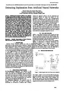
In using the traditional approaches (e.g. equations ( 1) and ( 5)), one is forced to adopt a linear or simple nonlinear form that must be explicitly designed by a researcher. Coe cients are then ® tted by traditional regression or simple numerical routines. If the researcher has not correctly envisioned all of the complex functional relationships between the input and output data, this approach will not work well. What is needed is a structure which adaptively develops its own basis functions, and their corresponding coe cients, from collected data. Neural networks have the ability to learn patterns or relationships given training data, and to generalize or extract results from the data (Anderson and Rosenfeld 1988, Wasserman 1989, Zornetzer et al. 1990 ). After training, the network is a machine that approximately maps inputs to the desired output(s). 3.1. T he structure of neural networks The approximation capability of neural networks is based on connectionism ( Fu 1994 ). A network’s structure consists of a number of processing nodes with weighted connections between these nodes. The multilayer perception (MLP) neural network in ® gure 1 shows the fundamental principles of many of the networks discussed in this paper. The network consists of multiple inputs (e.g. optical or radar signals), a single layer or multiple layers of hidden nodes, and a single layer of output nodes. The inputs are usually fully connected to the nodes in the hidden layer(s) which in turn are fully connected to output nodes. In addition, connections that bypass hidden layers are allowed. All signals ¯ ow from the input nodes through, or around, the hidden layer(s) to the output nodes (feed-forward ). No feedback processes are allowed. Each node (denoted as a circle) is a nonlinear processor of its input signals (® gure 2 ). Each node receives signals from previous nodes or from network input



2645

Figure 1. A neural network showing the fundamental principles of many of the networks discussed in this paper. The network consists of multiple inputs (e.g. optical or radar signals) , a single layer or multiple layers of hidden nodes, and a single layer of output nodes. The inputs are fully connected to the nodes in the hidden layer (s) which in turn are fully connected output nodes. All processing of signals ¯ ows from the input nodes through the hidden layer (s) to the output nodes (feed-forward ). No feedback processes are allowed. Each hidden node (denoted as circles) is a nonlinear processor of its input signals.

Figure 2. Each hidden node within a network is a nonlinear processor. Each node receives signals from previous nodes or from network input (e.g. optical or radar signals). The node then processes these signals and produces an output signal. The node in the ® gure has n input signals. Each input signal S i is weighted ( w i ). The total input signal I to a node is calculated as shown. The term b is the bias associated with the node. The weights and the bias term for each node are unique to that node and these terms are learned (optimized ) by the network. The output (O ) of the node is calculated as shown. f is the activation function, in many studies f is the sigmoid function.

(e.g. optical or radar signals). The node then processes these signals and produces an output signal. The node in the ® gure has n input signals. Each input signal S i is weighted (w i ). The total input signal I to a node, also called the net function ( Rumelhart et al. 1986 ), is I=

n

=

i 1

w i S i+b

( 6)

where b is the bias associated with the node. The weights and the bias term for each node are unique to that node and these terms are learned (optimized ) by the network.

2646

D. S. Kimes et al.

The knowledge contained in a network is encoded in the weights and biases. The output of a node is O =f (I )

or

O =f

A

n

=

i 1

w i S k+b

B

( 7)

where f is the activation function. In many studies f is the sigmoid function f (x )= 1/ 1+ eÕ x. Thus, when f is the sigmoid function equation ( 7 ) becomes O=

CA


1+ exp Õ

1

n

=

i 1

w i S i+b

BD

( 8)

The sigmoid function compresses all node output signals into the range 0± 1. This is necessary to prevent signal saturation and attenuation when the inputs are not bounded. In addition, it is a smooth function that permits calculation of gradients. The same type of activation function is generally applied to all hidden nodes in the network (® gure 1 ) as the signals are fed forward through the network. 3.2. Alternate structures A wide variety of neural network structures have been designed and applied to various applications, as reviewed by Lippman ( 1987 ) and Haykin ( 1994). In this paper, some of the common networks that have been used to extract continuous vegetation variables are mentioned. The MLP networks are the most well known and widely used networks. These networks display the fundamental principles of all the networks discussed in the previous section. A MLP network is a multilayer feedforward network ( ® gure 1 ). Another kind of network used in some studies has a cascade method of network construction ( Fahlmann and Lebiere 1988) that adds a hidden node one at a time during its training phase. As each hidden node is added it is fully connected to all previous nodes. Once a hidden node is added and trained its weights (® gure 2 ) are ® xed. The advantages of such a network are that it learns quickly, determines its own network size, and does not require the relatively slow backpropagation learning algorithm; such networks also seem to be robust in learning complex mapping functions relevant to the radiative transfer problem ( Kimes et al. 1996, 1997). 3.3. Important properties MLP neural networks have been shown to have desirable approximation properties by Cybenko ( 1989), Girosi and Poggio (1989 ), Hecht-Nielsen (1989 ), Chen and Manry ( 1990), Hartman et al. ( 1990), Hornik et al. ( 1990), and Fu (1994 ). Speci® cally, a three-layer network (input, hidden and output layers) as shown in ® gure 1 is su cient to approximate continuous functions arbitrarily well over a bounded compact set. Two speci® c examples of mapping are the operations of estimation and classi® cation from statistical signal processing. Recently, there have been some results that combine statistical signal processing theory and neural network theory. Neural net classi® ers have been shown to approximate Bayes discriminant by Ruck et al. ( 1990) and Wan ( 1990). MLP neural nets and Volterra ® lters ( Volterra 1887), which are nonlinear function approximators similar to functional link nets ( Pao 1989 ), have proven useful in estimation. They can be computationally e cient compared to conventional estimators, which are often brute force and iterative in nature. It has


2647


been shown by Manry et al. ( 1996 a) that feed-forward networks approximate the optimal minimum mean square estimator. Their approximation error variances are therefore governed by the Cramer± Rao maximum a posteriori bounds (CRM bounds). It has been shown that these bounds can be meaningful, even when the variables to be estimated are not Gaussian (Manry et al. 1996 b). 3.4. T raining Neural network training algorithms attempt to ® nd the best nonlinear approximation based on the network’s complexity and network structure without the constraint of linearity or pre-speci® ed nonlinearity used in regression analysis. This is an iterative process involving the modi® cation of the weights and biases and the evaluation of network error. These optimum weights and biases minimize the global error between the desired output and the actual output for all training patterns. Training patterns are input± output pairs that represent the `real’ world. Designing e cient and robust algorithms to ® nd the optimum weights and biases of networks is a critical aspect of neural network studies. This training process can be computationally intensive. However, the trained network can be applied with great speed to new input data (test data or ® eld data). In this case, the input data are introduced to the input layer and the output of each node of the network is calculated by applying equation ( 7) using the weights and biases determined during the training phase. The output from each node is propagated forward through the network until the ® nal output(s) of the network is(are) calculated. In this study, the outputs are continuous variables. The ® rst practical training algorithm was backpropagation ( Werbos 1974, 1994, Rumelhart et al. 1986 ). The backpropagation algorithm derives the network weights and biases (® gure 2 ) by using one version of steepest descent. In this study the inputs are typically optical or radar signals and any other ancillary data and the output(s) is(are) the variable(s) to be predicted. In most applications, the training time required for the backpropagation algorithm is long. E orts have been made to develop training techniques that are signi® cantly faster than the backpropagation algorithm. Many investigators have noted that linear equations can be solved for the output weights in the MLP. These investigators have developed algorithms which alternately solve for the output weights and improve the hidden unit weights. For example, Manry et al. ( 1994 ) and Dawson et al. ( 1993 ) presented several new training algorithms built upon an output weight optimization technique. These techniques were shown to be signi® cantly faster than the backpropagation algorithm. 3.5. Pruning of less usef ul units As with more traditional regression techniques, neural networks can produce models which under® t or over® t the data. A high training error (or inability to converge) is characteristic of under® tting. A high testing error is characteristic of over® tting. Ideally, one would like a close correspondence between the training and testing errors. Several methods can be used to avoid over® tting the training data. These techniques include reducing the network structure ( pruning or eliminating some hidden nodes), halting training when a test performance on independent data begins to decline, and transformation of the input variables. Several techniques have been used to improve the accuracy of neural networks. These techniques include numerical transformations of the input variables and input


2648

D. S. Kimes et al.

variable selection methods. Numerical transformations performed on the inputs often improve the performance of networks ( Tukey 1977, Chatterjee and Price 1991). Continuous transformation functions which may improve network performance include linear, log, exponential, square, fourth power, square root, inverse, inverse of the square, hyperbolic tangent functions, etc. Linear transformation of an input variable is always used, however, and other transformations of the input may be included as additional inputs. The transformations that produce distributions similar to the output variable of interest are those that may be useful in improving the accuracy of the network. Tukey ( 1977) and Chatterjee and Price ( 1991) discuss in detail the traits of transformations that may be useful and those that are de® nitely not useful. Jiang et al. ( 1994 ) developed methods for optimizing the network size (i.e. the number of hidden layers and nodes within a layer) of trained MLP neural networks. They modelled the network as a power series which allowed them to: ( 1) replace nodes from the network which can be approximated by zero or ® rst-degree polynomials; (2 ) measure the e ect of removing hidden layers; and ( 3) measure the degree of nonlinearity inherent in the trained network. This technique allows one to reduce the network size and analyse the network for advantages over conventional linear or multi-dimensional polynomial ® ts. 4.

Attributes of neural network extraction techniques

Neural networks have several attributes which facilitate the extraction of continuous vegetation variables from remotely sensed data. The advantages of neural networks as compared to traditional techniques are now discussed and studies that have made advances in this research area are reviewed. Neural network approaches have been shown to be equal or superior to conventional techniques, especially when strong nonlinear components exist in the system being studied ( Hewitson and Crane 1994, chapter 1 ). 4.1. Neural networks as initial models In many areas of research, physically based radiative scattering models do not exist or are not accurate. In cases where models are lacking, neural networks can provide the initial model. If accuracy is the only concern, then a neural network may be entirely adequate and desirable. A neural network can model the system on the basis of a set of encoded input/ output examples of the system. The network maps inputs to the desired output by learning the mathematical function underlying the system. With this method, input and output variables can be related without any knowledge or assumptions about the underlying mathematical representation. Several examples follow. Simpson ( 1994 ) used a neural network to predict crop yield. For many years the traditional method used to calculate crop yield was to develop a correlation between the cumulative NDVI index and the crop yield. The technique resulted in large errors in estimation (Simpson 1994). These simple traditional techniques can be greatly improved by including relevant ancillary information. In many cases, physically based crop yield models do not exist. Neural networks can provide accurate initial models in these cases. Simpson ( 1994 ) developed a network based on NDVI (derived from Thematic Mapper ( TM ) data), rainfall (monthly), hours of sunshine (monthly), temperature (monthly mean, minimum and maximum), and maximum soil moisture de® cit inputs. The standard error divided by the average yield was 5%. Pierce et al. ( 1994) used a MLP network as the initial model to predict trunk



2649

density, average trunk diameter, and average trunk height of Loblolly pine using AirSAR data ( P, L, and C bands with HH, VV, and HV polarizations). The network successfully predicted these variables with a worst-case error of 12% and an average error of 2%. As discussed in § 2, many transformations (ratios, indices, etc.) of optical and radar wavelengths are used to infer vegetation variables of interest. The goal of these studies is to ® nd the transformation that produces the maximum degree of accuracy when applied to a particular class of remote sensing problems. Researchers often use simple transformations (ratios, indices, etc.) because they are fast, easy to apply and well covered by the literature. However, they provide little if any physical insight that can be used e ectively to increase the accuracy of inference. Consequently, we propose that an adaptive learning technique such as a neural network would be superior to these simple transformations in many applications. Neural networks have the potential to learn more accurate relationships because they are not con® ned to the ® xed relationships represented by the above simple transformations. The neural network approach is free to learn complex relationships that could not be envisioned by researchers. However, neural networks do not provide any insight into physically based relationships between the dependent and independent variables (i.e. between output and inputs). As an example of the advantages of neural networks over vegetation index techniques the following example is presented. Baret et al. ( 1995 ) compared vegetation index techniques to a neural network approach for estimating the canopy gap fraction (nadir view) of sugar beet canopies using red and NIR re¯ ectances. Both ® eld data and simulated data from the SAIL model with hot spots ( Verhoef 1984, Kuusk 1991) and the PROSPECT model ( Jacquemoud and Baret 1990 ) were applied to each technique. The vegetation index technique used a simple nonlinear equation (equation ( 5)) as discussed in § 2.2. Equation ( 5) can be solved for parameters V Is , V I and K using a nonlinear optimization routine. Because of the inclusion of 2 equation ( 5 ), this index technique is more sophisticated and more accurate than most vegetation index techniques. Several vegetation indices were tested (SAVI, TSAVI, MSAVI, PVI, GEMI, and NDVI ) as well as a simple MLP network. The neural network approach generally performed signi® cantly better than the vegetation index techniques. For each of these vegetation index techniques, the researcher is adopting an equation form which is a combination of a linear transform (equation ( 1)) and a simple nonlinear equation (equation ( 5 )). Researchers are limited in the functional forms which are able to envisage. The neural network approach generally performed signi® cantly better because the neural network is free to learn functional relationships that could not be envisaged by the researchers. Kimes et al. ( 1996) used a MLP network as an initial model to extract forest age in a Paci® c Northwest forest using TM and topographic data. Understanding the changes of forest fragmentation through time are important for assessing alterations in ecosystem processes (forest productivity, species diversity, nutrient cycling, carbon ¯ ux, hydrology, spread of pests, etc.) and wildlife habitat and populations. The development of physically based radiative scattering models that incorporate forest growth and topography and that can be used to extract forest variables is in its infancy. Consequently, accurate models that are invertible in this context are lacking. Various MLP networks were trained and tested to predict forest age from TM data and topographic data ( Kimes et al. 1996 ). The results demonstrate that neural networks can be used as an initial model for inferring forest age. The best


2650

D. S. Kimes et al.

network used inputs of TM bands 3, 4, 5, elevation, slope and aspect. The RMS values (root mean square error of the predicted forest age versus true forest age) of the network were of the order of 5 years. Such studies serve as benchmarks for current and future modelling studies. Gopal and Woodcock ( 1996 ) developed a MLP to extract conifer mortality (represented as change in basal area) using TM data during a prolonged drought in Lake Tahoe Basin in California between 1988 and 1991. Inputs to the network were 2 TM bands 1± 5 for both a 1988 and 1991 scene. The R value ( between predicted and measured conifer mortality) and the RMS value were 0´89 and 6´80 respectively. The accuracy of this network was signi® cantly better than that obtained using traditional change detection techniques. For example, the accuracies obtained using the Gramm± Schmidt change detection approach (Collins and Woodcock 1995 ) were 2 between 0´48 and 0´70 for R , and between 9´91 and 7´85 for the RMS value. Gopal and Woodcock ( 1996 ) analysed why the neural network approach was signi® cantly better than the benchmark approach and found that the improvement was due to nonlinearities in the relationship between the spectral data and conifer mortality. Ultimately, the scienti® c community needs to develop physically based radiative scattering models for the above areas of research. These models need to be accurate and invertible for the desired variables. Until these activities mature, the neural network approach will provide an initial model for predicting vegetation variables. 4.2. Neural networks as baseline control A network can be used as a baseline control while developing adequate physically based models ( Fu 1994). Where adequate ® eld and ground data sets exist, a neural network can be trained and tested on these data sets. These networks attempt to ® nd the optimum functional relationships that exist between the input variables and the output variables of interest and can be trained in the forward direction on the ® eld data (e.g. vegetation canopy variables are the inputs and radiative scattering is the output). Improvements to the physically based model are advisable if it cannot surpass the accuracy of a neural network. Speci® cally, model accuracies less than neural network accuracies indicate that the physical processes embedded in the model must be improved (i.e. made more realistic). In this manner, neural networks provide a performance standard for evaluating current and future physically based models ( Fu 1994). 4.3. Neural networks for inverting physically based models In § 2.3 the di culties in inverting physically based models were discussed. In summary, the following di culties can occur when using numerical optimization techniques to invert models. These techniques can be time consuming and generally cannot be applied on a pixel-by-pixel basis for large regions. From a practical standpoint, it is often di cult to collect the measurements (multiple view angles and wavelengths) needed for an accurate inversion. Often models must be simpli® ed by decreasing the number of parameters and /or simplifying the radiative transfer function before a stable and accurate inversion can be developed. Simpli® ed models tend to be more inaccurate than the full models. Neural network approaches provide potential solutions to all or some of these problems. Signi® cant simpli® cations of physical models are made so that direct inversion using numerical techniques can be successfully applied. The disadvantage of this



2651

approach is that underlying relationships that may be useful in extracting the variables of interest may be deleted. In contrast, the neural network approach can be applied to the most sophisticated model without reducing the number of parameters or simplifying the physical processes. Models that have many parameters and include all physical processes tend to be the most accurate and robust models. Thus, the neural network approach applied to these models may, potentially, ® nd more optimal relationships between the desired input and output variables. This approach provides a sound bench mark in terms of accuracy for extracting various variables. If direct inversion techniques of simpli® ed models do not equal the accuracy obtained using the neural network approach on the full model, this signi® es that important underlying relationships are being deleted in the direct inversion approach. A neural network approach can be used to invert physically based models accurately and e ciently. The approach is as follows. The physically based model describes the mathematical relationships between all the vegetation and radiative parameters. The model is used to simulate a wide array of vegetation canopies (the range of all canopies that would be encountered in the application space) in the forward directionÐ that is, the vegetation canopy variables are the input and the radiative scattering above the canopy is calculated. Using the model a wide range of canopies and their associated directional re¯ ectances or backscatter values can be calculated. Using these model-based data, training and testing data sets can be constructed and presented to various neural networks. These data sets consist of pairs of data containing the desired network inputs (e.g. optical and /or radar) and the true outputs (e.g. vegetation variables of interest). Mathematical relationships between the inputs and the outputs are embedded in these data. In theory the neural network approximates the optimal underlying mathematical relationships used to map the inputs to the output. If only weak mathematical relationships between the input and output values exist then the network results will be poor. Thus, using this approach a neural network can be used to invert a model. This inversion scheme can be applied using input data that can be practically obtained in remote sensing missions. Many studies have successfully used this approach and are reviewed here. Chen et al. ( 1993 ) successfully used a MLP model to invert an active polarimetric microwave model of corn. A vector radiative transfer model with rough surface boundary conditions was used. The model results compared well with experimental data at L and C bands. The simultaneous inversion of three variables (corn height, volumetric moisture of corn stalks and volumetric soil moisture) was carried out using a MLP network. Inputs to the network were eight Muller matrix elements: M 11 , M 22 , M 33 and M 44 at both L and C bands. The accuracy of the neural network was high, with errors less than 10%. The accuracy was improved by using both the L and C bands and the Muller matrix elements M 33 and M 44 . These matrix elements contain phase di erence information between like polarizations. Smith ( 1993 ) used a MLP neural network to invert a multiple scattering model in the optical region. He developed networks to predict LAI from multiple spectral bands with accuracies comparable to ground observations and showed that this technique was robust when applied to varying soil backgrounds. Using a MLP network, Chuah (1993) inverted a Monte Carlo radar backscatter model to infer leaf moisture content and radius and thickness of a circular leaf. The vegetation layer was modelled as a half-space of randomly oriented and randomly distributed discs. The Monte Carlo model handles multiple scattering between the scatterers (Chuah and Tan 1989) and this model was used to simulate the radar


2652

D. S. Kimes et al.

backscatter coe cients, given the vegetation variables. Chuah and Tan trained two networks to invert the model for leaf moisture content. One network used a single frequency (1 GHz) with three view angles and three polarizations (HH, VV, HV ) for a total of nine inputs. This network had an accuracy of leaf moisture content to within Ô 2%. With the introduction of random noise to the inputs of Ô 1/2 dB and Ô 1 dB, the error in estimated leaf moisture content was less than Ô 5% and Ô 8% respectively. The second network used multifrequencies (1± 8 GHz with three view angles and three polarizations) and gave similar accuracies. Finally, a network was trained to estimate three variables simultaneously: leaf moisture content and the radius and thickness of the circular discs using the multifrequency data. The accuracy of this network for inferring plant moisture content and radius of the discs was approximately 8%, while the accuracy of inferring the thickness of the discs was within 10%. Pierce et al. ( 1994 ) used a MLP network for inverting the MIMICS model. The MIMICS model has been used successfully in predicting the radar response to vegetation canopies. The inputs to the network were the polarimetric backscatter values ( L and C bands with HH, VV, and HV polarizations) and the output was the desired variable (e.g. tree height, crown thickness, leaf density, etc.). Also included were ratios of some of the polarimetric backscatter terms. Aspen stands of di erent ages were modelled in the study. Using MLP networks, accurate inversions of these variables were achieved for the di erent stands of simulated aspen. Baret et al. ( 1995 ) successfully used a neural network to invert a combined optical model with hot spot e ects (SAIL model ( Verhoef 1984, Kuusk 1991)) and a leaf re¯ ectance / transmittance model ( PROSPECT model ( Jacquemoud and Baret 1990 )). The inputs were the simulated red and NIR re¯ ectances of sugar beet canopies and 2 the output was the canopy gap fraction in the nadir direction. The R value and the RMS error for the predicted versus true canopy gap fraction were 0´97 and 0´058 respectively. These results are generally better than traditional techniques. Kimes et al. ( 1997) used a neural network approach to invert a combined forest growth model and a radar backscatter model. The forest growth model captures the natural variations of forest stands (e.g. growth, regeneration, death, multiple species and competition for light). This model was used to produce vegetation structure data typical of northern temperate forests in Maine, USA. These data supplied inputs to the radar backscatter model which simulated the polarimetric radar backscatter (C, L, P, X bands) above the mixed conifer / hardwood forests. Using these simulated data, various neural networks were trained with inputs of di erent backscatter bands and output variables of total biomass, total number of trees, mean tree height and mean tree age. Techniques utilized included transformation of input variables, variable selection with a genetic algorithm and a cascade network. The accuracies ( RMS 2 and R values) for inferring various variables from radar backscatter were for total 2 1 biomass ( 1´6 kg mÕ , 0´94), number of trees ( 48 haÕ , 0´94), tree height ( 0´47 m, 0´88), and tree age ( 24´0 y, 0´83). The accuracy of these networks was therefore superior to traditional techniques. Several networks were shown to be relatively insensitive to the addition of random noise to radar backscatter. Abuelgasim et al. ( 1998) used a MLP network to invert the model of Li and Strahler ( 1992 ). This geometric optical model has been successful in predicting the bidirectional re¯ ectance of canopies as a function of the geometry and spatial distribution of trees/ shrubs, the component signatures of the canopy elements, and the illumination geometry. The model was used to generate input and output data from a conifer forest, savanna and shrubland. The inputs to the network were 18



2653

directional re¯ ectances consisting of nine views from the principal plane of the sun and nine views from across the principal plane of the sun. In addition, three component signatures and the solar illumination angle were inputs to the network. The output was the density of the canopy, crown shape of the trees/ shrubs, and canopy 2 height. The R values between the predicted canopy variables and the true canopy variables were 0´85, 0´75 and 0´75 respectively for density, crown shape and height. In this study and all of the studies mentioned above the trained neural networks act as e cient algorithms for inverting complex physically based models and require no estimation of unknown variables. Dawson ( 1994 ) suggested several steps in inverting physically based scattering models. One step is the selection of network inputs via a model sensitivity analysis. A sensitivity analysis identi® es input variables that are sensitive to the desired output. Presenting only sensitive variables to the network increases the probability that a global minimum can be found in the training phase. Fourty and Baret ( 1997) used a MLP to invert a coupled model ( leaf, soil, canopy and atmospheric models). The inputs to the MLP were simulated satellite re¯ ectance spectra within the 880± 2380 nm domain. Canopy-level variables (whole canopy water content, whole canopy dry matter content and LAI ) were retrieved accurately. Leaflevel variables (water content per unit leaf area and speci® c leaf weight) were retrieved with less accuracy. The neural networks demonstrated higher accuracies than multiple linear regression methods. Wang and Dong ( 1997) used MLPs to invert the Santa Barbra microwave canopy backscatter model for predicting forest stand density and dbh (tree trunk diameter at breast height ). This retrieval technique was tested using ground and AIRSAR backscatter data from two ponderosa pine forest stands near Mt Shasta, California. The RMS errors in retrieving the dbh and stand density for both stands were less 1 than or equal to 6´1 cm and 71´2 trees haÕ . 4.4. Neural networks for de® ning relevant variables Networks can be used as a variable selection tool to determine a set of variables that are relevant to the desired variable(s) to be inferred. If the mapping of a network is not accurate, then some input variable(s) could be missing. Furthermore, an input variable is relevant to the problem only if it signi® cantly increases the network’s performance. Alternately, if there is an unacceptably large number of input variables, several types of algorithms can be used to ® nd desirable subsets of input variables. Genetic algorithms ( Koza 1993 ) may be used to select an optimal subset of input variables. In this type of application, the genetic algorithm searches for a subset of input variables that behave synergistically to produce the highest network accuracy. The algorithm starts with a small subset of inputs of limited size and adds input variables according to the network performance. This evolutionary process is detailed by Koza ( 1993) and a speci® c application relevant to this paper is described by Kimes et al. ( 1997). In these ways, networks can be used to identify input variables which best predict the variable(s) of interest. Several examples follow. The network analysis in the forest age study discussed previously ( Kimes et al. 1996 ) de® ned a set of variables that were relevant to modelling e orts designed to infer forest age. Speci® cally it was discovered that the best inputs were TM bands 3, 4, 5, elevation, slope and aspect. TM bands 1, 2, 6, and 7 did not signi® cantly add information to the network for learning forest age. Furthermore, the study suggests that topographic information (elevation, slope and aspect ) can be e ectively utilized


2654

D. S. Kimes et al.

by a neural network approach. However, it was shown that this same topographic information was not useful when used in a traditional linear approach. Neural networks can also be applied to simulated data from physically based models to de® ne a set of variables which may be used to infer variable(s) of interest. As discussed previously, Kimes et al. ( 1997) used a neural network approach to develop accurate algorithms for inverting a complex forest backscatter model. Using these simulated data, various neural networks were trained with inputs of di erent backscatter bands and output variables of total biomass, total number of trees, mean tree height and mean tree age. The authors found that the networks that used only AIRSAR bands (C, L, P) had a high degree of accuracy. The inclusion of the X band with the AIRSAR bands did not seem to increase the accuracy of the networks signi® cantly. The networks that used only the C and L bands still had a relatively 2 high degree of accuracy for all forest variables (R values from 0´75 to 0´91). The signi® cance of this fact is that there is no current instrument or planned instrument that is collecting or will collect P band data. However, there are planned instruments 2 collecting C and L band data. Modest accuracies (R values from 0´65 to 0´84) were 2 obtained with networks that used only the L band and poor accuracies (R values from 0´36 to 0´46) were obtained with networks that used only the C band. In an alternate approach, it has been shown that optimal subsets of input variables can be identi® ed from smaller subsets by adding those inputs which reduce the CRM bounds the most. CRM bound calculation requires a model of the noisy inputs in terms of the desired outputs. Such models can include scattering or other known models plus Gaussian noise statistics (Apollo et al. 1992, Yu et al. 1993, Manry et al. 1996 c, Dawson et al. 1997 ). The CRM bounds have been extended to the case of non-Gaussian noise and parameters (Manry et al. 1996 b). Noise statistics, the input signal model, and the CRM bounds can also be found from neural network training data ( Liang et al. 1994). 4.5. Neural networks as adaptable systems Neural networks are readily adaptable. They can easily incorporate new ancillary information that would be di cult or impossible to use with conventional techniques. For example, Simpson ( 1994) used a neural network to predict crop yield. He used TM data ( NDVI values) along with monthly values of rainfall, hours of sunshine, temperature (mean, minimum and maximum) and maximum soil moisture de® cit. As new relevant information such as soil types, slopes, elevation, meteorological data, fertilizer methods, etc. becomes available, it can easily be incorporated into the neural network (Simpson 1994). New input variables can be introduced to the network and tested with ease. Incorporation of new ancillary information is di cult with conventional algorithms. Simpson ( 1994 ) noted that a signi® cant advantage of neural networks in estimating crop yield is their ability to improve the accuracy of crop yield forecasts continually by simply collecting more data and introducing it to the network for training. Kimes et al. ( 1996 ) included topographic data (slope, aspect, elevation) as ancillary information to infer forest age from TM data. They found that by introducing this ancillary information the network accuracy improved signi® cantly (from 8´0 y to 5´1 y root mean error squared). It was not known how to incorporate topographic information e ectively using traditional techniques. However, neural networks are ideally suited to learning new relationships between ancillary information, other input variables and the desired output variable. New input variables can be



2655

introduced to the network and tested with ease. This is especially useful when a researcher expects a new variable to add information to the problem of interest but does not have any knowledge of the functional form to use in introducing the new variable using traditional techniques. Traditional numerical methods have di culty in inverting multiple disconnected models. For example, Ranson et al. ( 1997 ) used a forest growth model to simulate growth and development of northern mixed coniferous hardwood forests. The output from this model was used as input to the canopy backscatter model that calculated radar backscatter coe cients for simulated forest stands. Classic numerical inversion of such a disconnected system (multiple models) is di cult when the functional connection between the di erent models is not explicitly de® ned. In these situations, researchers often adopt simple linear or nonlinear forms. For example, Ranson et al. ( 1997) chose to develop a simple relationship (equation ( 1 ) with transformations) to infer forest biomass from the radar backscatter coe cients. Neural networks are ideally suited for such problems. Networks ® nd the best nonlinear function based on the network’s complexity without the constraint of linearity or pre-speci® ed nonlinearity used in traditional techniques. No explicit functional relationships between the disconnected models are required. Kimes et al. ( 1997 ) found that networks were signi® cantly more accurate than traditional techniques for inverting the disconnected models of Ranson et al. ( 1997). Potentially, a combination of disparate wavelength regions can improve the accuracy of vegetation variable extraction. Di erent wavelength regions are sensitive to di erent vegetation variables. Theoretically, a synergism may be realized by combining these disparate wavelength regions, resulting in an improvement in the extraction of vegetation variables. However, radiative transfer models that combine, for instance, both optical and radar bands in one coherent model do not exist. Consequently, classical inversions using optical and radar wavelengths simultaneously cannot be performed. Most studies are forced to use traditional methods. For example, Hame and Solli (1994 ) applied a regression analysis to predict forest stand variables ( proportion of deciduous trees and tree stem volume) from TM, Advanced Very High Resolution Radiometer (AVHRR), and ERS-1 Synthetic Aperture Radar (SAR) data. Neural networks are ideally suited for providing an initial model for e ectively combining di erent wavelength regions. Networks have the potential of learning new optimum relationships using measured data or data from several di erent physically based models (e.g. an optical model and a radar backscatter model ). The di erent models can be used to generate data independently for the di erent wavelength regions. These data sets can be presented to the networks for training and testing. Networks can also accept as training data a combination of both measured and simulated data. The ¯ exibility of neural networks to accept combinations of measured and model-based data from di erent sources can be powerful and e ective in remote sensing missions. Although a number of studies have used neural networks to fuse optical and radar regions and perform classi® cations of data (e.g. Butini et al. 1992 ) little work on the extraction of continuous vegetation variables has been reported in the literature. 5.

New advances in neural network algorithms

5.1. Complexity estimation One of the principal di culties in designing neural networks for estimation and classi® cation is that the required complexity of the networks is unknown. Here, the


2656

D. S. Kimes et al.

complexity is de® ned in two parts as ( 1) the number of network weights and thresholds and ( 2 ) the network structure or topology in terms of the number of layers, units per layer and connectivity. Recently, two groups have attempted to use Akaike’s Information Criterion (AIC) (Akaike 1974) to estimate neural network size. Fogel ( 1991 ) applied the AIC to neural network classi® ers for two classes. Another group (Murata et al. 1994 ) applied the AIC to determine the required size of neural network estimators. Both approaches ( 1) use the minimum mean-square training error E * for each candidate network size, ( 2) use the number of network weights N w , and ( 3) require the training of hundreds or thousands of neural networks of various sizes. Both approaches are therefore impractical for determining the required neural network size in a reasonable amount of time, because of point ( 2). A third group of investigators ( Kim and Manry 1995) has developed a fast method for predicting the required MLP size. In this approach a nearest neighbour estimator ( NNE) is designed which has one output vector per cluster. As the NNE is iteratively trained using a relevant set of training data, more clusters are added and the training mean square error ( MSE) decreases. The predicted MLP structure at each iteration is a MLP which is theoretically capable of memorizing the NNE’s clusters and output vectors. At each iteration, the predicted MSE is that of the corresponding NNE. This approach is possible and worthwhile because: ( 1) training of a NNE is almost an order of magnitude faster than MLP training algorithms; ( 2) once trained, the MLP can be applied to data one or more orders of magnitude faster than the NNE’s; ( 3) a MLP can closely approximate the performance of a NNE if it can process the NNE’s cluster vectors without error (memorize the clusters and their associated output vectors); and ( 4 ) a MLP or Volterra ® lter can memorize as many patterns as it has free parameters per output node (its complexity) (Gopalakrishnan et al. 1994). 5.2. Modular networks Modular networks break a desired mapping down into simpler ones which are approximated separately and then recombined. There are many di erent ways to connect simple modules together to form a working network. In some approaches the modules are cascaded ( Rohani and Manry 1991, 1994 ). In others, the modules operate in parallel ( Hrycej 1990, Nowlan 1990, Jacobs and Jordan 1993). In an alternate parallel structure (Subbarayan et al. 1996), an input pattern is routed to only one of the many parallel modules for processing, thereby reducing the computations required to process an input vector. In all of these approaches, highly accurate mappings are obtained in a fraction of the time required to train a MLP. 5.3. Automated network design The remaining problems which have prevented the widespread acceptance of neural network technology include: ( 1 ) the di culty in determining the required network size or complexity; ( 2) the long training time required; and ( 3) the di culty in determining whether or not training has converged. Each of these problems has been addressed separately in the literature and in this paper. However, what is needed is a system which solves all three problems simultaneously. Such a system is being developed and has been applied to the short-term power load forecasting problem (Manry et al. 1996 c) and to data from remote sensing problems (Manry 1995 ). This system uses a complexity estimation algorithm to size the network ( Kim


2657

and Manry 1995 ), a fast training algorithm to obtain a small training error ( Manry et al. 1994 ), and a pruning algorithm to reduce network complexity and promote generalization ( Jiang et al. 1994 ).


6.

Conclusions and implications

E orts are being made to develop e cient algorithms that incorporate a wide variety of spectral data with other available ancillary data for extracting continuous vegetation variables. Inferring continuous variables implies that functional relationships must be made among the predicted variable(s), the remotely sensed data and the ancillary data. Neural networks have attributes which facilitate the extraction of vegetation variables. Neural networks have signi® cant advantages as compared to traditional techniques when applied to both measurement and modelling studies. In many areas of research, physically based radiative scattering models do not exist or are not accurate. In cases where accurate models are lacking, neural networks can be used as the initial model. If accuracy is the only concern then a neural network may be entirely adequate and desirable. A neural network can model the system on the basis of a set of encoded input/ output examples of the system. The network maps inputs to the desired output by learning the mathematical function underlying the system. Using this approach, input and output variables can be related without any knowledge or assumptions concerning the underlying mathematical representation. Neural networks can provide a baseline against which the performance of physically based models can be compared. The networks can be trained on ® eld data. Improvements to the physically based model are indicated if it cannot surpass the accuracy of a neural network. Speci® cally, model accuracies less than neural network accuracies indicate that the physical processes embedded in the model must be expanded and /or improved (i.e. made more realistic). In this manner, neural networks provide a performance standard for evaluating current and future physically based models. In many of the studies cited in this paper a physical modelling approach is necessary for realistic applications that span the entire range of vegetation conditions of interest. However, to actually use physically based models for extracting vegetation variables, the models must be inverted. In most cases these models are complex nonlinear systems which must be solved using numerical methods. The following di culties can occur when using numerical optimization techniques to invert models. These techniques are computationally intensive and generally cannot be applied on a pixel-by-pixel basis for large regions. From a practical standpoint, often it is di cult to collect the measurements (for example, multiple view angles and wavelengths) needed for an accurate inversion. Often models need to be simpli® ed before a stable and accurate inversion can be obtained. The models are simpli® ed by decreasing the number of parameters and /or simplifying the radiative transfer function. However, simpli® ed models tend to be less accurate than the full models. Neural network approaches provide potential solutions to all or some of these problems. The neural network approach can be applied to the most sophisticated model without reducing the number of parameters or simplifying the physical processes. The models that have many parameters and include all physical processes tend to be the most accurate and robust models. Thus, the application of neural networks to invert these models has the potential of ® nding more optimal relationships between the desired input and output variables. This approach provides a sound benchmark


2658

D. S. Kimes et al.

in terms of accuracy for extracting various variables. If direct inversion techniques of simpli® ed models do not equal the accuracy obtained using the neural network approach on the full model then important underlying relationships are being deleted in the direct inversion approach. Networks can be used as a variable selection tool to de® ne a set of variables which accurately predict variable(s) of interest. If the mapping of a network is not accurate, then perhaps some input variables are missing. Also an input variable is relevant to the problem only if it signi® cantly increases the network’s performance. Thus, networks can be used to identify relevant variables for physically based modeling development. Neural networks are readily adaptable. They can easily incorporate new information that would be di cult or impossible to use with conventional techniques. Neural networks are ideally suited to learning new relationships among ancillary information, other input variables and the desired output variable. New input variables can be introduced to the network and tested easily. This is especially useful when a researcher expects a new variable to add information to the problem of interest but does not have any knowledge of the functional form to use in introducing the new variable using traditional techniques. Neural networks attempt to ® nd the best nonlinear function based on the network’s complexity without the constraint of linearity or pre-speci® ed nonlinearity which is required in regression analysis. Neural networks represent a much more powerful and adaptive nonlinear equation form. This power and ¯ exibility is gained by repeating nonlinear activation functions in a network structure. This unique structure allows the neural network to learn complex functional relationships between the input and output data that cannot be envisaged by a researcher. Acknowledgement

This work was funded in part by the Ecological Process and Modeling Program, O ce of Mission to Planet Earth, NASA Headquarters. References A buelgasim, A . A ., G opal, S ., and S trahler, A . H ., 1998, Forward and inverse modeling of canopy directional re¯ ectance using a neural network. International Journal of Remote Sensing 19, 453± 471. A kaike, H ., 1974, A new look at the statistical model identi® cation. IEEE T ransactions on Automatic Control , 19, 716± 723. A nderson, J . A ., and R osenfeld, E . , (editors), 1988, Neurocomputing: Foundations of Research,

(Cambridge, MA: MIT Press).

A pollo, S . J ., M anry, M . T ., A llen, L . S ., and L yle, W . D ., 1992, Optimality of transforms for parameter estimation. Conference Record of the T wenty-Sixth Annual Asilomar Conference on Signals, Systems, and Computers, October 1992 ( Piscataway, NJ: IEEE),

vol. 1 pp. 294± 298.

A srar, G ., and D ozier, J ., 1994, EOSÐ

Science Strategy for the Earth Observing System , ( Woodbury, New York: AIP Press). A srar, G ., and G reenstone, R ., (editors), 1995, MTPE EOS Reference Handbook. EOS Project Science O ce, NASA / GSFC, Greenbelt, Maryland, USA. A tkinson, P . M ., and T atnall, A . R . L . , 1997, Neural networks in remote sensing. International Journal of Remote Sensing, 18, 699± 709. A ttema, E . P . W ., and U laby, F . T . , 1978, Vegetation modeled as a water cloud. Radio Science, 13, 357± 364. B aret, F ., C levers, J . G . P . W ., and S teven, M . D ., 1995, The robustness of canopy gap



2659

fraction estimates from red and near-infrared re¯ ectances: a comparison of approaches. Remote Sensing of Environment , 54, 141± 151. B utini, F ., C appellini, V ., and F ini, S ., 1992, Remote sensing data fusion on intelligent terminals. European T ransactions on T elecommunications and Related T echnologies , 3, 555± 563. C hatterjee, S ., and P rice, B . , 1991, Regression Analysis by Example ( New York: Wiley). C hen, M . S ., and M anry, M . T . , 1990, Back-propagation representation theorem using power series. Proceedings of International Joint Conference on Neural Networks (IJCNN) 90, San Diego, California 17± 21 June 1990 (Piscataway, NJ: IEEE), pp. I-643± I-648. C hen, Z ., T sang, L ., K uga, Y ., and C han, C . , 1993, Active polarimetric microwave remote sensing of corn and multiparametric retrieval of corn parameters with an arti® cial neural network. Microwave and Optical T echnology L etters, 6, 611± 615. C huah, H . T . , 1993, An arti® cial neural network for inversion of vegetation parameters from radar backscatter coe cients. Journal of Electromagnetic Waves and Applications , 7, 1075± 1092. C huah, H . T ., and T an, H . S ., 1989, A Monte Carlo method for radar backscatter from a half-space random medium. IEEE T ransactions on Geoscience and Remote Sensing, 27, 86± 93. C ollins, J . B ., and W oodcock, C . E . , 1995, Change detection using the Gramm± Schmidt transformation applied to mapping forest mortality. Remote Sensing of Environment , 50, 267± 279. C ybenko, G ., 1989, Approximations by superpositions of a sigmoidal function. Mathematical Control, Signals, and Systems, 2, 303± 314. D awson, M . S ., 1994, Applications of electromagnetic scattering models to parameter retrieval and classi® cation. In Microwave Scattering and Emission Models and T heir Applications , chapter 12, edited by A. K. Fung. ( Norwood, MA: Artech House). D awson, M . S ., F ung, A . K ., and M anry, M . T . , 1993, Surface parameter retrieval using fast learning neural networks. Remote Sensing Reviews, 7, 1± 18. D awson, M . S ., F ung, A . K ., and M anry, M . T . , 1997, A robust statistical-based estimator for soil moisture retrieval from radar measurements. IEEE T ransactions on Geoscience and Remote Sensing, 35, 57± 67. D obson, M . C ., U laby, F . T ., L e T oan, T ., B eaudoin, A ., K asischke, E . S ., and C hristensen, N . L . J r , 1992, Dependence of radar backscatter on coniferous forest biomass. IEEE T ransactions on Geoscience and Remote Sensing, 30, 412± 415. D obson, M . C ., U laby, F . T ., P ierce, L . E ., S harik, T . L ., B ergen, K . M ., K ellndorfer, J ., K endra, J . R ., L i, E ., L in, Y . C ., N ashashibi, A ., S arabandi, K ., and S iqueira, P ., 1995, Estimation of forest biophysical characteristics in Northern Michigan with SIRC / XSAR. IEEE T ransactions on Geoscience and Remote Sensing, 33, 877± 895. D raper, N . R ., and S mith, H ., 1966, Applied Regression Analysis (New York: Wiley). F ahlmann, S ., and L ebiere, C . , 1988, The cascade-correlation learning architecture. In Advances in Neural Information Processing Systems, vol. 2, edited by D. Touretzky (Aan Mateo, CA: Morgan Kaufmann), pp. 524± 532. F ogel, D . B . , 1991, An information criterion for optimal neural network selection. IEEE T ransactions on Neural Networks, 2, 490± 497. F ourty, T ., and B aret, F . , 1997, Vegetation water and dry matter contents estimated from top-of-the-atmosphere re¯ ectance data: a simulation study. Remote Sensing of Environment , 61, 34± 45. F u, L . , 1994, Neural Networks in Computer Intelligence ( New York: McGraw-Hill ). F ung, A . K ., 1994, Microwave Scattering and Emission Models and T heir Applications ( Norwood, MA: Artech House). G ao, B . C . , 1996, NDWIÐ a normalized di erence water index for remote-sensing of vegetation liquid water from space. Remote Sensing of Environment , 58, 257± 266. G irosi, F ., and P oggio, T . , 1989, Representation properties of networks: Kolmogorov’ s theorem is irrelevant. Neural Computation , 1, 465± 469. G oel, N ., 1987, Models of vegetation canopy re¯ ectance and their use in estimation of biophysical parameters from re¯ ectance data. Remote Sensing Reviews, 3, 1± 212. G opal, S ., and W oodcock, C . , 1996, Remote sensing of forest change using arti® cial neural networks. IEEE T ransactions on Geoscience and Remote Sensing, 34, 398± 404.

2660

D. S. Kimes et al.

G opalakrishnan, A ., J iang, X ., C hen, M .-S ., and M anry, M . T . , 1994, Constructive proof of e cient pattern storage in the multilayer perceptron. Conference Record of the T wenty-Seventh Annual Asilomar Conference on Signals, Systems, and Computers ,

November 1994 (Piscataway, NJ: IEEE), vol. 1, pp. 306± 390.


G ovaerts, Y ., and V erstraete, M . M . , 1994, Evaluation of the capability of BRDF models

to retrieve structural information on the observed target as described by a threedimensional ray tracing code. Proceedings of the Society of Photo-Optical Instrumentation Engineers, 2314, 9± 20. G oward, S . N ., M arkham, B ., D ye, D . G ., D ulaney, W ., and Y ang, J ., 1991, Normalized di erence vegetation index measurements from the advanced very high resolution radiometer. Remote Sensing of Environment , 35, 257± 277. G utman, G . G ., 1991, Vegetation indices from AVHRR: an update and future prospects. Remote Sensing of Environment , 35, 121± 136. H all, F . G ., T ownshend, J . R ., and E ngman, E . T . , 1995, Status of remote sensing algorithms for estimation of land surface state parameters. Remote Sensing of Environment , 51, 138± 156. H ame, T ., and S alli, A ., 1994, Estimation of forest stand characteristics using Landsat TM, NOAA AVHRR, ERS-1 SAR, and other image data. Proceedings of the Society of Photo-Optical Instrumentation Engineers, 2314, 233± 243. H artman, E . J ., K eeler, J . D ., and K owalski, J . M . , 1990, Layered neural networks with Gaussian hidden units as universal approximations. Neural Computation , 2, 210± 215. H aykin, S ., 1994, Neural Networks, A Comprehensive Foundation (New York: Macmillan). H echt- N ielsen, R ., 1989, Theory of backpropagation neural networks. Proceedings of International Joint Conference on Neural Networks (IJCNN)’89, Washington D.C., 18± 22 June 1989 (Piscataway, NJ: IEEE), vol. 1, pp. I-593± I-605. H ewitson, B . C ., and C rane, R . F . , 1994, Looks and uses. In Neural Nets: Applications in Geography , edited by B. C. Hewitson and R. C. Crane ( Dordrecht: Kluwer). H ornik, K ., S tinchcombe, M ., and W hite, H ., 1990, Universal approximation of an unknown mapping and its derivatives using multilayer feedforward networks. Neural Networks, 3, 551± 560. H rycej, T . , 1990, A modular architecture for e cient learning. Proceedings of International Joint Conference on Neural Networks (IJCNN)’90, San Diego, California 8± 12 July 1990 (Piscataway, NJ: IEEE), vol. I, pp. I-557± I-562. H uete, A . R ., 1988, A soil-adjusted vegetation index (SAVI). Remote Sensing of Environment , 25, 295± 309. H uete, A . R ., J ackson, R . D ., and P ost, D . F . , 1985, Spectral response of a plant canopy with di erent soil backgrounds. Remote Sensing of Environment , 17, 37± 53. H uete, A . R ., J ustice, C ., and L iu, H ., 1994, Development of vegetation and soil indices for MODIS-EOS. Remote Sensing of Environment , 49, 224± 234. J acobs, R . A ., and J ordan, M . I ., 1993, Learning piecewise control strategies in a modular neural network architecture. IEEE T ransactions on Systems, Man, and Cybernetics, 23, 337± 345. J acquemoud, S ., 1993, Inversion of the PROSPECT + SAIL canopy re¯ ectance model from AVIRIS equivalent spectraÐ theoretical study. Remote Sensing of Environment , 44, 281± 292. J acquemoud, S ., and B aret, F . , 1990, PROSPECT: a model of leaf optical properties spectra. Remote Sensing of Environment , 34, 75± 91. J akubauskas, M . E . , 1996, Thematic mapper characterization of Lodgepole Pine seral stages in Yellowstone National Park, USA. Remote Sensing of Environment , 56, 118± 132. J iang, X ., C hen, M ., M anry, M . T ., D awson, M . S ., and F ung, A . K ., 1994, Analysis and optimization of neural networks for remote sensing. Remote Sensing Reviews, 9, 97± 114. K asischke, E . S ., B ourgeau-C havez, L . L ., C hristensen, N . L . J r and D obson, M . C . , 1991, The relationship between above ground biomass and radar backscatter observed on airborne SAR imagery. Proc. T hird AIRSAR Workshop, NASA, JPL , Pasadena, California, May 1991 , edited by J. J. van Zyl, pp. 11± 21. K asischke, E . S ., C hristensen, N . L . J r and B ourgeau-C havez, L . L . , 1995, Correlating radar backscatter with components of biomass in Loblolly pine forests. IEEE T ransactions on Geoscience and Remote Sensing, 33, 643± 659.


2661

K aram, M . A ., F ung, A . K ., L ang, R . H ., and C hauhan, N . S ., 1992, A microwave scattering model for layered vegetation. IEEE T ransactions on Geoscience and Remote Sensing, 30, 767± 784. K aufman, K . J ., and T anre, D ., 1992, Atmospherically resistant vegetation index for EOSMODIS. IEEE T ransactions on Geoscience and Remote Sensing, 30, 261± 270. K im, K . K ., and M anry, M . T . , 1995, A complexity algorithm for estimating the size of the multilayer perceptron. Conference Record of the T wenty-Ninth Annual Asilomar Conference on Signals, Systems, and Computers 29 October± 1 November 1995


( Piscataway, NJ: IEEE), vol. 2, pp. 899± 903.

K imes, D . S ., H olben, B . N ., N ickeson, J . E ., and M c K ee, A ., 1996, Extracting forest age in a Paci® c Northwest forest from thematic mapper and topographic data. Remote Sensing of Environment , 56, 133± 140. K imes, D . S ., R anson, K . J ., and S un, G ., 1997, Inversion of a forest backscatter model using neural networks. International Journal of Remote Sensing, 18, 2181± 2199. K oza, J ., 1993, Genetic Programming (Cambridge, MA: MIT Press). K uusk, A ., 1991, The hot spot e ect in plant canopy re¯ ectance. In Photo-V egetation Interaction. Applications in Optical Remote Sensing and Plant Ecology, edited by R. B.

Myneni and J. Ross (Berlin: Springer-Verlag ), pp. 139± 159.

K uusk, A ., 1994, Multispectral canopy re¯ ectance model. Remote Sensing of Environment , 50, 75± 82. L eprieur, C ., V erstraete, M . M ., P inty, B ., and C hehbouni, A ., 1994, NOAA / AVHRR

vegetation indices: suitability for monitoring fractional vegetation cover of the terrestrial biosphere. Physical measurements and signatures in Remote Sensing, Sixth Symposium of International Society of Photogrammetric and Remote Sensing, V al d’Isere, France, 17± 21 January 1994 , pp. 1103± 1110. L e T oan, T ., B eaudoin, A ., R iom, J ., and G uyon, D ., 1992, Relating forest biomass to SAR data. IEEE T ransactions on Geoscience and Remote Sensing, 30, 403± 411. L i, X ., and S trahler, A . H ., 1992, Geometric optical bidirectional re¯ ectance modeling of the discrete crown vegetation canopy: e ects of crown chape and mutual shadowing. IEEE T ransactions on Geoscience and Remote Sensing, 30, 276± 292. L iang, W ., M anry, M . T ., Y u, Q ., A pollo, S . J ., D awson, M . S ., and F ung, A . K ., 1994, Bounding the Performance of neural network estimators, given only a set of training data. Conference Record of the T wenty-Eighth Annual Asilomar Conference on Signals, Systems, and Computers 31 October± 2 November 1994 (Piscataway, NJ: IEEE), vol. 2, pp. 912± 916. L ippman, R . P ., 1987, An introduction to computing with neural nets. IEEE ASSP Magazine , April, 4± 22. M anry, M . T . , 1995, A self-organizing system for the development of neural network parameter estimators. IEEE Workshop on Neural Networks for Signal Processing (NNSP ’95), Cambridge, Massachusetts 31 August± 2 September 1995 , pp. 105± 114. M anry, M . T ., A pollo, S . J ., and Y u, Q ., 1996 a, Minimum mean square estimation and neural networks. Neurocomputing , 13, 59± 74. M anry, M . T ., D awson, M . S ., F ung, A . K ., A pollo, S . J ., A llen, L . S ., L yle, W . D ., and G ong, W . , 1994, Fast training of neural networks for remote sensing. Remote Sensing Reviews, 9, 77± 96. M anry, M . T ., H sieh, C .-H ., A pollo, S . J ., D awson, M . S ., and F ung, A . K ., 1996 b, Cramer ± Rao maximum a posteriori bounds for non-Gaussian signals and parameters. International Journal of Intelligent Control and Systems, 1, 381± 391. M anry, M . T ., S hoults, R ., and N accarino, J ., 1996 c, An automated system for developing neural network short term load forecasters. Proceedings of the 58th American Power Conference, Chicago, Illinois, April 9 ± 11, 1996 (Chicago, IL: Illinois Institute of Technology), vol. 1, pp. 237± 241. M oghaddam, M . , 1994, Retrieval of forest canopy parameters for OTTER. Proceedings of the Society of Photo-Optical Instrumentation Engineers, 2314, 549± 558. M c D onald, K . C ., and U laby, F . T . , 1993, Radiative transfer modeling of discontinuous tree canopies at microwave frequencies. International Journal of Remote Sensing, 14, 2097± 2128. M urata, N ., Y oshizawa, S ., and A mari, S ., 1994, Network information criterion-determinin g


2662

D. S. Kimes et al.

the number of hidden units for an arti® cial neural network model. IEEE T ransactions on Neural Networks, 5, 865± 872. M yneni, R . B ., H all, F . G ., S ellars, P . J ., and M arshak, A . L . , 1995, The interpretation of spectral vegetation indices. IEEE T ransactions on Geoscience and Remote Sensing, 33, 481± 486. M yneni, R . B ., and R oss, J ., 1991, Photon± V egetation Interactions ( New York: SpringerVerlag). M yneni, R . B ., R oss, J ., and A srar, G ., 1989, A review on the theory of photon transport in leaf canopies. Agricultural Forest Meteorology , 45, 1± 153. N owlan, S . J ., 1990, Maximum likelihood competitive learning. In Advances in Neural Information Processing Systems, vol. 2, edited by D. S. Touretzky, pp. 574± 582. P ao, Y .-H . , 1989, Adaptive Pattern Recognition and Neural Networks (New York: AddisonWesley). P ierce, L . E ., S arabandi, K ., and U laby, F . T . , 1994, Application of an arti® cial neural network in canopy scattering inversion. International Journal of Remote Sensing, 15, 3263± 3270. P inty, B ., and V erstraete, M . M . , 1991, Extracting information on surface properties from bidirectional re¯ ectance measurements. Journal of Geophysical Research, 96, 2865± 2874. P inty, B ., and V erstraete, M . M . , 1992, GEMI: A non linear index to monitor global vegetation from satellites. V egetation , 101, 15± 20. P inty, B ., V erstraete, M . M ., and D ickinson, R . E . , 1990, A physical model of the bidirectional re¯ ectance of vegetation canopies. 2. Inversion and validation. Journal of Geophysical Research, 95, 11767± 11775. P olatin, P . F ., S arabandi, K ., and U laby, F . T . , 1994, An iterative inversion algorithm with application to the polarimetric radar response of vegetation canopies. IEEE T ransactions on Geoscience and Remote Sensing, 32, 62± 71. P revot, L ., and S chmugge, T . , 1994, Combined use of theoretical and semi-empirical models of radar backscatter to estimate characteristics of canopies. Physical Measurements and signatures in Remote Sensing, Sixth Symposium of International Society of Photogrammetric and Remote Sensing, V al d’Isere, France, 17± 21 January 1994 , pp. 415± 430. P rivette, J . L ., M yneni, R . B ., and E mery, W . J ., 1996, Optimal sampling conditions for estimating grassland parameters via re¯ ectance model inversions. IEEE T ransactions on Geoscience and Remote Sensing, 34, 272± 284. P rivette, J . L ., M yneni, R . B ., T ucker, C . J ., and E mery, W . J ., 1994, Invertibility of a 1-D discrete ordinates canopy re¯ ectance model. Remote Sensing of Environment , 48, 89± 105. Q i, J ., and K err, Y . H ., 1994 a, On current compositing algorithms. Physical Measurements and Signatures in Remote Sensing, Sixth Symposium of International Society of Photogrammetric and Remote Sensing, V al d’Isere, France, 17± 21 January 1994 , pp. 135± 142. Q i, J ., K err, Y . H ., and C hehbouni, A ., 1994 b, External factor consideration in vegetation index development. Physical Measurements and Signatures in Remote Sensing, Sixth Symposium of International Society of Photogrammetric and Remote Sensing, V al d ’Isere, France, 17± 21 January 1994 . R anson, K . J ., and S un, G ., 1994, Mapping biomass of a northern forest using multifrequency SAR data. IEEE T ransactions on Geoscience and Remote Sensing, 32, 388± 396. R anson, K . J ., S un, G ., W eishampel, J . F ., and K nox, R . G ., 1997, Forest biomass from combined ecosystem and radar backscatter modeling. Remote Sensing of Environment , 59, 118± 133. R ignot, E ., W ay, J ., W illiams, C ., and V iereck, L . , 1994, Radar estimates of above ground biomass in boreal forest of interior Alaska. IEEE T ransactions on Geoscience and Remote Sensing, 32, 1117± 1124. R ohani, K ., and M anry, M . T . , 1991, The design of multi-layer perceptrons using building blocks. Proceedings of International Joint Conference on Neural Networks (IJCNN) 91, Seattle, Washington (Piscataway, NJ: IEEE), pp. II-497± II-502. R ohani, K ., and M anry, M . T . , 1994, Multi-layer neural network design based on a modular concept. Journal of Arti® cial Neural Networks, 1, 349± 370.


2663


R oss, J . K ., and M arshak, A . L . , 1989, In¯ uence of leaf orientation and the specular component of leaf re¯ ectance on the canopy bidirectional re¯ ectance. Remote Sensing of Environment , 24, 213± 225. R ouse, J . W ., H aas, R . H ., S chell, J . A ., D eering, D . W ., and H arlan, J . C . , 1974,

Monitoring the vernal advancement of retrogradation of natural vegetation. Type III, Final report, NASA / GSFC, Greenbelt, Maryland, USA. R uck, D . W . , 1990, The multilayer perceptron as an approximation to a Bayes optimal discriminant function. IEEE T ransactions on Neural Networks, 1, 296± 306. R umelhart, D . J ., H inton, G . E ., and W illiams, R . J ., 1986, Learning representations by back-propagation errors. Nature , 323, 533± 536. S aatchi, S . S ., and M oghaddam, M . , 1994, Biomass distribution in boreal forest using SAR imagery. Proceedings of the Society of Photo-Optical Instrumentation Engineers, 2314, 437± 447. S impson, G ., 1994, Crop yield prediction using a CMAC neural network. Proceedings of the Society of Photo-Optical Instrumentation Engineers, 2315, 160± 171. S mith, J . A ., 1993, LAI inversion using a back-propagation neural network trained with a multiple scattering model. IEEE T ransactions on Geoscience and Remote Sensing, 31, 1102± 1106. S ubbarayan, S ., K im, K . K ., M anry, M . T ., D evarajan, V ., and C hen, H .-H ., 1996, Modular neural network architecture using piece-wise linear mapping. Conference Record of the T hirtieth Annual Asilomar Conference on Signals, Systems, and Computers, 3± 6 November 1996 ( Piscataway, NJ: IEEE), vol. 2, pp. 1171± 1175. S un, G ., and R anson, K . J ., 1995, A three-dimensional radar backscatter model of forest canopies, IEEE T ransactions on Geoscience and Remote Sensing, 33, 372± 382. T ukey, J ., 1977, Exploratory Data Analysis (Reading, MA: Addison-Wesley). U laby, F . T ., A llen, C . T ., E ger, G ., and K anemasu, E . , 1984, Relating microwave backscatter coe cients to leaf area index. Remote Sensing of Environment , 14, 113± 133. U laby, F . T ., S arabandi, K ., M c D onald, M ., W hitt, M ., and D obson, M . C . , 1990, Michigan microwave canopy scattering model (MIMICS). International Journal of Remote Sensing, 11, 1123± 1253. V erhoef, W . , 1984, Light scattering by leaf layers with application to canopy re¯ ectance modeling: the SAIL model. Remote Sensing of Environment , 16, 125± 141. V olterra, V . , 1887, Sopra le funzioni che dipendono da altre funzioni. Rend. Regia Academia dei L ince, 20 Sem., pp. 97± 105, 141± 146, 153± 158. W an, E . A ., 1990, Neural network classi® cation: a Bayesian interpretation. IEEE T ransactions on Neural Networks, 1, 303± 305. W ang, Y ., and D ong, D ., 1997, Retrieving forest stand parameters from SAR backscatter data using a neural network trained by a canopy backscatter model. International Journal of Remote Sensing, 18, 981± 989. W asserman, P . D ., 1989, Neural Computing: T heory and Practice ( New York: Van Norstrand Reinhold ), p. 230. W erbos, P . J ., 1974, Beyond regression: new tools for prediction and analysis in the behavioral sciences. PhD Thesis, Harvard University, Cambridge, MA, USA. W erbos, P . J ., 1994, T he Roots of Backpropagati on: From Ordered Derivative to Neural Networks and Political Forecasting ( New York: Wiley). Y u, Q ., A pollo, S . J ., and M anry, M . T . , 1993, MAP estimation and the multilayer perceptron. Proceedings of the 1993 IEEE W orkshop on Neural Networks for Signal Processing, L inthicum Heights, Maryland, 6± 9 September 1993 , pp. 30± 39. Z ornetzer, S . F ., D avis, J . L ., and L au, C . , 1990, An Introduction to Neural and Electronic Networks ( New York: Academic).

Attributes of neural networks for extracting continuous ...

Attributes of neural networks for extracting continuous ...

Suggest Documents

Deep BLSTM Neural Networks for Unconstrained Continuous ...

Neural Networks and Continuous Time

Neural Networks and Continuous Time

Extracting Stochastic Machines from Recurrent Neural Networks ...

Extracting Explanation from Artificial Neural Networks - CiteSeerX

Extracting Explanation from Artificial Neural Networks - international ...

Deep neural networks for extracting baum-welch statistics for speaker ...

Continuous Neural Networks - Proceedings of Machine Learning

Using Deep Neural Networks for Extracting Sentiment ...

Lipschitz Continuous Neural Networks On L_P - CiteSeerX

Statistical Discretization of Continuous Attributes

Continuous-Time Recurrent Neural Networks for Generative - CiteSeerX

Discretizing Continuous Attributes While Learning

Efficient Learning of Continuous Neural Networks Abstract ... - CiteSeerX

Continuous attractor neural networks - Faculty of Computer Science

The Most General Framework of Continuous Hopfield Neural Networks

Ontology Based Automatic Attributes Extracting ... - Semantic Scholar

Extracting structural attributes from IKONOS imagery for ... - CiteSeerX

Neural networks applications for multimedia processing - Neural

Discretization of Continuous Attributes for Learning Classification Rules

Spiking Neural Networks As Continuous-Time Dynamical Systems ...

Tracking Changing Stimuli in Continuous Attractor Neural Networks

Adaptive and Variational Continuous Time Recurrent Neural Networks

Discretization of Continuous Attributes for Learning Classification Rules