Automated Alphabet Reduction Method with Evolutionary Algorithms for Protein Structure Prediction
Jaume Bacardit, Michael Stout, Jonathan D. Hirst, Kumara Sastry, Xavier Llor` a and Natalio Krasnogor IlliGAL Report No. 2007015 April 2007
Illinois Genetic Algorithms Laboratory University of Illinois at Urbana-Champaign 117 Transportation Building 104 S. Mathews Avenue Urbana, IL 61801 Office: (217) 333-2346 Fax: (217) 244-5705
Automated Alphabet Reduction Method with Evolutionary Algorithms for Protein Structure Prediction Jaume Bacardit1 , Michael Stout1 , Jonathan D. Hirst2 , Kumara Sastry3 , Xavier Llor` a4 and Natalio Krasnogor1 1
2
ASAP research group, School of Computer Science and IT, University of Nottingham, Jubilee Campus, Nottingham, NG8 1BB, UK jqb,mqs,
[email protected] 3
Illinois Genetic Algorithms Laboratory University of Illinois at Urbana-Champaign 104 S. Mathews Ave. Urbana, IL 61801
[email protected]
School of Chemistry University of Nottingham, University Park, Nottingham NG7 2RD, UK
[email protected]
4
National Center for Supercomputing Applications University of Illinois at Urbana-Champaign 1205 W.Clark Street, Urbana, IL 61801, USA
[email protected]
April 30, 2007 Abstract This paper focuses on automated procedures to reduce the dimensionality of protein structure prediction datasets by simplifying the way in which the primary sequence of a protein is represented. The potential benefits of this procedure are faster and easier learning process as well as the generation of more compact and human-readable classifiers. The dimensionality reduction procedure we propose consists on the reduction of the 20-letter amino acid (AA) alphabet, which is normally used to specify a protein sequence, into a lower cardinality alphabet. This reduction comes about by a clustering of AA types accordingly to their physical and chemical similarity. Our automated reduction procedure is guided by a fitness function based on the Mutual Information between the AA-based input attributes of the dataset and the protein structure feature that being predicted. To search for the optimal reduction, the Extended Compact Genetic Algorithm (ECGA) was used, and afterwards the results of this process were fed into (and validated by) BioHEL, a genetics-based machine learning technique. BioHEL used the reduced alphabet to induce rules for protein structure prediction features. BioHEL results are compared to two standard machine learning systems. Our results show that it is possible to reduce the size of the alphabet used for prediction from twenty to just three letters resulting in more compact, i.e. interpretable, rules. Also, a protein-wise accuracy performance measure suggests that the loss of accuracy acrued by this substantial alphabet reduction is not statistically significant when compared to the full alphabet.
1
Introduction
One of the main open problems in computational biology is the prediction of the 3D structure of protein chains, known as Protein Structure Prediction (PSP). Solving this domain is computationally very expensive due to its size and difficulty. For instance, one of the PSP predictors that obtained top results in the last CASP (Critical Assessment of Techniques for Protein Structure 1
Prediction) experiment was the Rosetta@home system (Misura, Chivian, Rohl, Kim, & Baker, 2006) which used a massive collaborative computing system to predict protein structures with up to 10000 computing days per protein. One of the possible ways in which PSP can be tackled is by using a divide-and-conquer approach where the problem of predicting the tertiary structure of a given sequence is split up into smaller challenges such as predicting secondary structure, solvent accessibility, coordination number, etc. Another, complementary, approach would be to reduce the size of the alphabet of the variables that are involved in the prediction of tertiary structure. An example of a high cardinality alphabet that can have its size reduced is the primary sequence of a protein that consist of a 20-letter alphabet representing the 20 natural amino acids (AA). An example of a widely explored alphabet reduction option is to transform the 20 letters AA alphabet into a two letters hydrophobic/polar (HP) alphabet. This reduction is usually followed by constraining the residue locations of the predicted protein to those of a 2D/3D lattice (Yue, Fiebig, Thomas, Sun, Shakhnovich, & Dill, 1995; Krasnogor, Blackburne, Burke, & Hirst, 2002), although sometimes this HP alphabet reduction is applied to real non-constrained proteins. A recent paper (Stout, Bacardit, Hirst, Krasnogor, & Blazewicz, 2006) compared the performance of several learning methods applied to predicting the coordination number for lattice-based proteins, real proteins with either HP alphabet or AA alphabet. The experiments showed that there is a significant although not big performance gap between the HP and AA alphabets. Moreover, the criterion to divide the AA types between hydrophobic and polar was the one of Broome and Hecht (Broome & Hecht, 2000), although there are alternative HP assignment policies (Mandel-Gutfreund & Gregoret, 2002) as well as real-valued hydrophobicity scales (Cornette, Cease, Margalit, Spouge, Berzofsky, & DeLisi, 1987). Several interesting questions related to alphabet reduction for protein structure prediction are: Is is possible to obtain statistically similar performance between the original AA alphabet and another alphabet with reduced number of symbols? Moreover, can we tailor the alphabet reduction criteria to each specific problem we want to solve? That is, shall we use the same reduce alphabet for, lets say, predicting coordination number and disulfide bridges? The aim of this paper is to answer these two questions. We propose an automated method to perform alphabet reduction. This method uses the Extended Compact Genetic Algorithm (Harik, 1999) to optimize the distribution of the 20 letters of the AA alphabet into a predefined number of categories. We apply this alphabet reduction to the coordination number prediction domain. For the fitness function of such reduction process we have chosen a rigorous information theory measure, the Mutual Information (Cover & Thomas, 1991). This measure relates the dependence between two variables, in this case the input attributes and the predicted class of the coordination number domain. By optimizing this measure we are looking for the alphabet reduction criterion that maintains as much as possible the useful information existing in the input attributes related to the predicted feature. We have performed experiments trying to reduce the AA alphabet into two, three, four and five groups and verified the performance of the reduction criteria by using the reduced alphabet on a separate learning task and comparing the predictive performance with the reduced alphabet versus the one obtained by using the original 20-letters alphabet. The learning process used BioHEL (Bioinformatics-Oriented Hierarchical Evolutionary Learning) (Bacardit & Krasnogor, 2006), a recent Learning Classifier System. We have also analyzed the relation between the resulting groups of attributes and some standard categories in which amino acids can be grouped (Betts & Russell, 2003). For comparison purposes we have also used other standard machine learning methods. The rest of the paper is structured as follows: Section 2 will contain a brief summary of background information and related work. Section 3 will describe all techniques used for the optimiza2
tion and learning stages of the experiments reported in the paper, while section 4 will describe the dataset and experimental setup. Section 5 will report the results of the experiments. Finally, section 6 will describe the conclusions and further work.
2
Background and related work
Proteins are heteropolymer molecules constructed as a chain of residues or amino acids of 20 different types. This string of amino acids is known as the primary sequence. In its native state, the chain folds to create a 3D structure. It is thought that this folding process has several steps. The first step, called secondary structure, consists of local structures such as alpha helix or beta sheets. These local structures can group in several conformations or domains forming a tertiary structure. Secondary and tertiary structure may form concomitantly. The final 3D structure of a protein consists of one or more domains. In this context, the coordination number (CN) of a certain residue is a profile of the end product of this folding process. That is, in the native state each residue will have a set of spatial nearest neighbours. The number of nearest neighbours of a given residue is its contact number. Some of these contacts can be close in the protein chain but other can be quite far apart. Some trivial contacts such as those with the immediate neighbour residues in the sequence are discarded. Figure 1 contains a graphical representation of the CN of a residue for an alpha helix, given a minimum chain separation (discarded trivial contacts) of two. In this example, the CN is two. This problem is closely related to contact map (CM) prediction that predicts, for all possible pairs of residues of a protein, if they are in contact or not. Figure 1: Graphical representation of the CN of a residue
There is a large literature in CN and CM prediction, in which a variety of machine learning paradigms have been used, such as linear regression (Kinjo, Horimoto, & Nishikawa, 2005), neural networks (Baldi & Pollastri, 2003), a combination of self-organizing maps and genetic programming (MacCallum, 2004), support vector machines (Zhao & Karypis, 2003), or learning classifier systems (Bacardit, Stout, Krasnogor, Hirst, & Blazewicz, 2006; Stout, Bacardit, Hirst, Krasnogor, & Blazewicz, 2006). Recent years have seen a renewed interest in alphabet reduction techniques as applied to PSP (Meiler, Zeidler, & Schm¨ahke, 2001; Melo & Marti-Renom, 2006; Mintseris & Weng, 2004; Stout, Bacardit, Hirst, Krasnogor, & Blazewicz, 2006). One example of a previous application of an Evolutionary Algorithm for alphabet reduction is (Melo & Marti-Renom, 2006). In this case, a GA
3
was used to optimize a reduction into 5 letters applied to sequence alignment. The fitness function was based on maximizing the difference between the sequence identity of the training alignments and a set of random alignments based on the same sequences. Another approach (Mintseris & Weng, 2004) applies Mutual Information to optimize alphabet reduction for contact potentials. This approach is very tailored to the problem being solved because the mutual information is computed between AA types (or AA groups) potentially in contact. Finally, Meiler et al. (Meiler, Zeidler, & Schm¨ahke, 2001) propose a slightly different approach. Instead of treating the AA types at a symbolic level, they characterize them numerically with several physical features and then apply a neural network to generate a lower dimensionality representation of these features.
3
Evolutionary computation methods and fitness function
The experiments reported in this paper have two stages. In the first one, ECGA is used to optimize the alphabet reduction mapping given the number of symbols of the final alphabet by using Mutual Information as fitness function. In the second stage, BioHEL is used to validate the reliability of the alphabet groupings found by ECGA by predicting over the reduced dataset.
3.1
Extended Compact Genetic Algorithm
Extended Compact Genetic Algorithm (Harik, 1999) is an optimization method belonging to the family of Estimation of Distribution Algorithms (Larranaga & Lozano, 2002). This method iteratively optimizes a population of candidate solutions by first heuristically estimating the structure of the problem being solved and later recombining the population based on this structure. The structure of the problem in ECGA is defined as non-overlapping groups of variables that interact among them. A greedy approach using a fitness function based on the Minimum Description Length (MDL) principle (Rissanen, 1978) applied to a type of probabilistic models called Marginal Product Models is used to find these groups of variables. The recombination of the population uses uniform crossover based on the identified structure. Specifically we use the χ-ary version of ECGA (de la Ossa, Sastry, & Lobo, 2006), adapted to use non-binary nominal variables, and the code is an slightly modified version of the one available at ftp://www-illigal.ge.uiuc.edu/pub/src/ECGA/chiECGA.tgz. The default parameters of ECGA were used except for the population size that was set up to 40000 individuals when optimizing the alphabet reduction for two or three letters, and 40000 when optimizing for four or five letters.
3.2
The BioHEL learning system
BioHEL (Bioinformatics-oriented Hierarchical Evolutionary Learning) is Genetics–Based Machine Learning (GBML) system following the Iterative Rule Learning or Separate-and-Conquer approach (F¨ urnkranz, 1999), first used in the GBML field by Venturini (Venturini, 1993). BioHEL is strongly influenced by GAssist (Bacardit, 2004) which is a Pittsburgh GBML system. Several of BioHEL features have been inherited from GAssist. The system applies an almost standard generational GA, which evolves individuals that are classification rules. The final solution of the learning process is a set of rules that is obtained by applying iteratively a GA. After each rule is obtained, the training examples that are covered by this rule are removed from the training set, to force the GA of the next iteration to explore other areas of the search space. The rules are inserted into a rule set with an explicit default rule that covers the majority class of the domain. The evolved rules will cover all the other classes. Therefore, the stopping 4
criteria of the learning process is when it is impossible to find any rule where the associated class is not the majority class of the matched examples. When this happens, all remained examples are assigned to the default rule. Also, several repetitions of the GA with the same set of instances are performed, and we will only insert in the rule set (and therefore remove examples from the training set) the best rule from all the GA runs. Each individual is a rule, which consists of a predicate and an associated class. We use the GABIL (DeJong & Spears, 1991) knowledge representation for the predicates of these rules. The system also uses a windowing scheme called ILAS (incremental learning with alternating strata) (Bacardit, Goldberg, Butz, Llor`a, & Garrell, 2004) to reduce the run-time of the system, especially for dataset with hundreds of thousands of instances, as in this paper. This mechanism divides the training set into several non-overlapping subsets and chooses a different subset at each GA iteration for the fitness computations of the individuals. The fitness function of BioHEL is based on the Minimum Description Length (MDL) principle (Rissanen, 1978). The MDL principle is a metric applied to a theory (a rule) which balances its complexity and accuracy. BioHEL MDL formula is adapted from GAssist one as follows: F itness = T L · W + EL
(1)
where T L stands for theory length (the complexity of the solution) and EL stands for exceptions length (the accuracy of the solution). This fitness function has to be minimized. W is a weight that adjusts the relation between T L and EL. BioHEL uses the automatic weight adjustment heuristic proposed for GAssist (Bacardit, 2004). The parameters of this heuristic are adjusted as follows: Initial TL ratio: 0.25, weight relax factor: 0.90, max iterations without improvement: 10. T L is defined as follows: Pi=N A
T L(R) =
i=1
N umZeros(Ri )/Cardi NA
(2)
where R is a rule, N A is the number of attributes of the domain, Ri is the predicate of rule R associated to attribute i, NumZeros counts the number of bits set to zero for a given predicate in GABIL representation and Cardi is the cardinality of attribute i. T L always has a value between 0 and 1. It has been designed in this way in order to simplify the tuning of W . The number of zeros in the GABIL predicates are a measure of specificity. Therefore, promoting the minimization of zeros means promoting general and thus less complex rules. The design of EL has to take into account a suitable trade off between accuracy and coverage thus covering as many examples as possible without sacrificing accuracy. To this end, our proposed coverage measure is initially biased towards covering a certain minimum of examples and once a given coverage threshold has been reached the bias is reduced. The measure is defined as follows:
EL(R) = 2 − ACC(R) − COV (R) corr(R) ACC(R) = matched(R) (
COV =
RC M CR · CB M CR + (1 − M CR) ·
RC−CB 1−RC
If RC < CB If RC ≥ CB
RC =
5
matched(R) |T |
(3) (4) (5) (6)
COV is the adjusted coverage metric that promotes the coverage of at least a certain minimum number of examples, while RC is the raw coverage of the rule. ACC is the accuracy of the rule, corr(R) is the number of examples correctly classified by R, matched(R) is the number of examples matched by R, M CR is the weight given in the coverage formula to achieving the minimum coverage, CB is the minimum coverage threshold and |T | is the total number of training examples. For all the tests reported in the paper, M CR has 0.9 value, and CB has value 0.01. Finally, we have used a mechanism wrapped over BioHEL to boost its performance. We generate several rule sets using GAssist with different random seeds and combine them as an ensemble, combining their predictions using a simple majority vote. This approach is similar to Bagging (Breiman, 1996). BioHEL used the values for the parameters defined in (Bacardit, 2004) except for the followings: population size 500; GA iterations 200; repetitions of rule learning: 2; rule sets per ensemble; 10.
3.3
Mutual Information
The aim of the alphabet reduction optimization is to simplify the representation of the dataset in a way that maintains the underlying information that is really needed for the learning process. Therefore, the fitness function for such a process should give an estimation of what can the reduced input information tell about the output. Ideally, we could simply learn the reduced dataset generated by each individual that we evaluate and use the training accuracy as fitness function, but this option is not feasible due to the enormous computational cost that would be required. Therefore, we need to use some cheap estimation of the relationship between inputs and output as fitness function, and we have chosen the Mutual Information metric for this task. The mutual information is an information theory measure that quantifies the interrelationship that two discrete variables have among each other (Cover & Thomas, 1991), that is, how much information can one variable tell about the other one. The mutual information is defined as follows: I(X; Y ) =
X X y∈Y xinX
p(x, y)log
p(x, y) p(x)p(y)
(7)
Where p(x) and p(y) are the probabilities of appearance of x and y respectively and p(x, y) is the probability of having x, y at the same time. In our specific case, we use the mutual information to measure the quantity of information that the input variables of the alphabet-reduced dataset have in relation to the classes on the domain. That is, for a given instance, x represents a string that concatenates the input variables of the instance, while y encodes the associated class for that instance.
4
Problem definition and experimental design
4.1
Problem definition
The dataset that we have used in this paper is the one identified as CN1 with two states and uniform length class partition criteria in (Bacardit, Stout, Krasnogor, Hirst, & Blazewicz, 2006). Its main characteristics are briefly described as follows: 4.1.1
Coordination number Definition
The CN definition is the one proposed by Kinjo et al. (Kinjo, Horimoto, & Nishikawa, 2005). The distance used is defined using the Cβ atom (Cα for glycine) of the residues. Next, the boundary of 6
the sphere around the residue defined by the distance cutoff dc ∈ 2 X
(8)
where rij is the distance between the Cβ atoms of the ith and jth residues. The constant w determines the sharpness of the boundary of the sphere. The dataset used in this paper had a distance cutoff dc of 10 ˚ A. The real-valued definition of CN has been discretized in order to transform the dataset into a classification problem that can be mined by BioHEL. The chosen discretization algorithm is the well-known unsupervised uniform-length (UL) discretization. Moreover, for the experiments of this paper we have used the simplest version of the dataset, dividing the domain into two states, low or high CN. 4.1.2
Protein dataset
We have used the dataset and training/test partitions proposed by Kinjo et al. The protein chains were selected from PDB-REPRDB (Noguchi, Matsuda, & Akiyama, 2001) with the following conditions: less than 30% of sequence identity, sequence length greater than 50, no membrane proteins, no nonstandard residues, no chain breaks, resolution better than 2 ˚ A and a crystallographic R factor better than 20%. Chains that had no entry in the HSSP (Sander & Schneider, 1991) database were discarded. The final data set contains 1050 protein chains and 257560 residues. 4.1.3
Definition of the training and tests sets
The set was divided randomly into ten pairs of training and test set using 950 proteins for training and 100 for test in each set, using bootstrap. The proteins included in each partition are reported in http://maccl01.genes.nig.ac.jp/~akinjo/sippre/suppl/list/. The definition of the input attributes is the one identified as CN1 in (Bacardit, Stout, Krasnogor, Hirst, & Blazewicz, 2006). The input data will consist of the AA type of the residues in a window around the target one. A window size of 4 (4 residues at each side of the target) has been used. Therefore, each instance consist of 9 nominal attributes of cardinality 21 (the 20 AA types plus the symbol that represents end of chain, in case that the window overlaps with the beginning or the end of a protein chain). Figure 2 contains a representation of the windowing process that creates the instances of the dataset.
7
Sequence (AA,CN): (S,0),(K,0), (Y,0),(V,0),(D,0),(R,0),(V,1), (I,0),(A,0),(E,0) X,X,X,X,S,K,Y,V,D 0 X,X,X,S,K,Y,V,D,R 0 X,X,S,K,Y,V,D,R,V 0 X,S,K,Y,V,D,R,V,I 0 Instances S,K,Y,V,D,R,V,I,A 0 K,Y,V,D,R,V,I,A,E 0 Y,V,D,R,V,I,A,E,V 1 V,D,R,V,I,A,E,V,E 0 D,R,V,I,A,E,V,E,K 0 R,V,I,A,E,V,E,K,K 0
Figure 2: Representation of the windowing process used to generate the instances of the dataset 4.1.4
Performance measure
In section 5 we will report the performance of the learning process of BioHEL over the reduced datasets in two different ways. On one hand we will use the standard machine learning accuracy metric (#correct examples/#total examples) (called residue-wise accuracy). On the other hand, as usual in the protein structure prediction field (Kinjo, Horimoto, & Nishikawa, 2005), we will take into account the fact that each example (a residue) belongs to a protein chain. Therefore, we will first compute the standard accuracy measure for each protein chain, and then average these accuracies to obtain the final performance measure (called protein-wise accuracy). Because different chains have different lengths, residue-wise accuracy and protein-wise accuracy can differ greatly. The rationale for reporting the second measure is to mimic the real-life situation, in which a new protein is sequenced, and researchers are interested in the predicted properties based on the entire protein sequence, independent of its length.
4.2 4.2.1
Experimental design Steps of the experimental process
The following protocol was used for our experiments: • For alphabet size = 2 to 5 do: 1. ECGA is used to find the optimal alphabet reduction of size alphabet size based on the MI-based fitness function. 2. The alphabet reduction policy is applied to the dataset 3. BioHEL, C4.5 and Naive Bayes are applied to learn the dataset with optimal reduced alphabet For comparison purposes we have used two more learning algorithms as well al BioHEL. We chose two simple and fast methods as C4.5 (Quinlan, 1993) and Naive Bayes (John & Langley, 1995), using the implementation from the WEKA package (Witten & Frank, 2000) of both of them. 4.2.2
Representation and fitness function of the alphabet reduction process
The chromosome optimized by ECGA is very simple. It has one gene for each letter of the original alphabet (the 20 AA types plus the end-of-chain symbol) meaning the group of letters where this 8
AA type is assigned. This gene can take a value from the range 0..N − 1, where N is the predefined number of symbols of the reduced alphabet. Table 1 illustrates an example of such chromosome for a reduction process into two groups. Orig. Alphabet Genotype Phenotype
ACDEFGHIKLMNPQRSTVWXY 001100001001111110010 Group 1: ACF GHILM V W Y Group 2: DEKN P QRST X
Table 1: Representation of the chromosome for the alphabet reduction process for a two-letter reduction Each fitness computation follows these steps: 1. The reduction mappings are extracted from the chromosome 2. The instances of the training set are transformed into the low cardinality alphabet based on the extracted mappings 3. The mutual information between class attribute and the string formed by concatenating the input attributes is computed 4. This mutual information is the fitness value of the chromosome
5 5.1
Results Results of the alphabet reduction process
ECGA was used to find reductions to alphabets of two, three, four and five symbols; the results are reported in Table 2. ECGA was used to find alphabet reductions into two, three, four and five symbols alphabet. Table 2 describes the obtained reductions. For a better visualization of the physical properties of the AA groups obtained, we have painted each AA type using a different colour accordingly to the properties discussed in (Betts & Russell, 2003). The colored groups are further described in table 2. Table 2: Alphabet reductions generated by ECGA #letters 2 3 4 5
Groups of letters ACFGHILMVWY DEKNPQRSTX ACFILMVWY DEKNPQRX GHST AFHTY CILMV DEKPQX GNRSW AIS CHLV DEPQY FGMWX KNRT CLV - hydrophobic AIM - hydrophobic FWY - aromatic, neutral, hydrophobic DE - negatively charged KHR - positively charged
9
When optimizing for a two letters alphabet, the MI-based optimization process ends up finding two groups of AA types that separate the most hydrophobic residues (ACF GHILM V W Y ) from the rest. Hydrophobicity is one of the main factors in the folding process of proteins, so it is natural that a reduction process into only two symbols is equivalent to identifying the hydrophobic residues. From the experiment with three-letter alphabets we can observe that one of the groups still contains all-hydrophobic AA types (ACF ILM V W Y ) while the other two groups contain more mixed AA types. From the visualization of the obtained groups with colours we can see how only two of the colour groups (CLV and DE) are conserved across all reduced alphabet sizes. The colour mix for four-letter and five-letter alphabets is considerable, meaning that the obtained groups have very mixed physical properties difficult to explain and, as next subsection will show, make the problem more difficult to learn.
5.2
Validation of the reduced alphabets
The reduced alphabets were used to represent the datasets, and then the selected learning methods were applied over them. First of all, table 3 contains several results for BioHEL, such as the two studied accuracy measures (reside-wise and protein-wise) and statistics about the complexity of the solutions (in rules and expressed attributes per rule). As a baseline, results for BioHEL learning the original dataset with full AA type representation (labelled Orig.) are also included. These results were analyzed using statistical t-tests (95% conf.) to determine if the accuracy differences were significant, using the Bonferroni correction for multiple comparisons. The tests determined that the original dataset with AA alphabet significantly outperformed the representations with two and five letter alphabets for protein-wise accuracy and all of the reduced datasets for residue-wise accuracy. The rule sets obtained from all the reduced alphabets were more compact than the dataset using the AA type representation. Figure 3 contains a rule set obtained from the original dataset with full AA representation, while figure 4 contains a rule-set using the 2-letter alphabet, being much more simple and human-readable. Table 3: Residue-wise accuracy (RWA), Protein-wise accuracy (PWA), ave. rule set size and ave number of expressed attributes per rule of BioHEL applied to the reduced datasets. • marks the cases where the reduced dataset had significantly worse performance than the original dataset with AA type representation #letters Orig. 2 3 4 5
RWA 74.0±0.5 72.3±0.5• 73.0±0.6• 72.6±0.6• 72.0±0.6•
PWA 77.0±0.7 75.8±0.7• 76.4±0.7 76.1±0.8 75.7±0.8•
#rules 22.5±1.8 11.3±0.6 16.7±1.4 15.4±1.3 14.6±1.5
#expr. att./rule 8.88±0.34 5.39±0.49 5.95±0.98 6.18±1.17 6.93±1.05
Based on existing work (Stout, Bacardit, Hirst, Krasnogor, & Blazewicz, 2006) we expected that the reduction into two groups would suffer from a significant performance degradation as the alphabet reduction simplifies the input data substantially thus inevitably losing some information. Moreover, as the number of groups increases, we expected to see a reduction of the performance gap between reduced and original alphabet. Interestingly, this new experimental results show that, contrary to our expectations, the reduced dataset with higher performance is the one with three groups. Moreover, we also note that a higher number of symbols does not help increasing the performance. 10
1:If AA−4 ∈ / {E, N, Q, R, W }, AA−3 ∈ / {D, E, N, P, Q, R, S, X}, AA−2 ∈ / {E, P, S}, AA−1 ∈ / {D, E, G, K, N, P, Q, T }, AA ∈ {A, C, F, I, L, M, V, W }, AA1 ∈ / {D, E, G, P, Q}, AA2 ∈ / {D, H, K, P }, AA3 ∈ / {D, E, K, N, P, Q, R, S, T }, AA4 ∈ {A, C, F, G, I, L, M, V } then class is 1 2:If AA−4 ∈ / {T, X}, AA−3 ∈ / {E, N }, AA−2 ∈ / {E, K, N, Q, R, S, T }, AA−1 ∈ / {D, E, G, K, N, P, Q, R, S}, AA ∈ {C, F, I, L, V }, AA1 ∈ {C, F, G, I, L, M, V, W, X, Y }, AA2 ∈ / {E, K, N, P, Q, R}, AA3 ∈ / {E, K, P, R}, AA4 ∈ / {E, K, Q, X} then class is 1 . . . 18:If AA−4 ∈ / {E, K, N, P, X}, AA−3 ∈ {G, I, L, M, V, W, X, Y }, AA−2 ∈ / {D, E, K, N, P, Q, R, S}, AA−1 ∈ / {E, K, N, P, Q, R}, AA ∈ / {D, E, K, N, P, Q, R, S, T }, AA1 ∈ / {D, E, K, L, Q}, AA2 ∈ / {D, E, L}, AA3 ∈ / {D, K, M, N, P, Q, T }, AA4 ∈ / {C, N, T, X} then class is 1 19:Default class is 0
Figure 3: Rule-set obtained by BioHEL over the dataset with full AA type representation. AA±X means AA type for residue in position ±X in respect to the target residue 1:If AA−1 ∈ {0}, AA ∈ {0}, AA1 ∈ {0}, AA2 ∈ {0}, AA3 ∈ {0}, AA4 ∈ {0} then class is 1 2:If AA−3 ∈ {0}, AA−2 ∈ {0}, AA−1 ∈ {0}, AA ∈ {0}, AA3 ∈ {0}, AA4 ∈ {0} then class is 1 . . . 10:If AA−3 ∈ {0}, AA ∈ {0}, AA1 ∈ {0}, AA2 ∈ {0}, AA3 ∈ {0} then class is 1 11:Default class is 0
Figure 4: Rule-set obtained by BioHEL over the dataset with 2-letter alphabet representation. Letter 0 = ACFGHILMVWY, Letter 1 = DEKNPQRSTX. AA±X means the group of AA types for residue in position ±X in respect to the target residue A natural question that arises from these results is why reduced alphabets produce the above phenomena? Our hypothesis is that the mutual Information measure is not a robust enough fitness measure for this dataset. Table 4 contains the number of unique instances (inputs+output) and unique input vectors for the different reductions of the dataset. We can see how the datasets with four or five letters present a unique number of instance or inputs which is at least 64% of the dataset, meaning that there are many chances that there is a single instance representing certain unique inputs (thus, p(X) in the MI formula becomes 1/|T | in most cases). Mutual Information needs redundancy in order to estimate properly the relation between inputs and outputs, and there is almost no redundancy in the signal generated by the dataset. If the fitness function cannot provide appropriate guidance we cannot rely much on the obtained results. This is probably the reason why it is difficult to extract physical explanations from the groups of AA types that ECGA finds and, therefore, why it is not possible to obtain good performance when learning the reduced dataset. In this reduction process we have lost too much information by forming wrong groups of AA types. Table 4: Counts of unique instances and unique input vectors for the training fold 0 of the dataset # letters 2 3 4 5
Unique inputs 512 19254 150914 219943
Unique instances 1024 33839 175156 224747
Moreover, table 5 contains the accuracy obtained by the three tested learning algorithms. From 11
the table we can see how BioHEL, with the exception of the dataset with only two letters (and with very minor performance difference) is the method that reacts better to the alphabet reduction procedure as is able to obtain higher accuracy in most alphabet sizes as well as in the original 20-letter alphabet, showing its robustness. It is interesting to note that C4.5 is the only method that obtains higher accuracy in one of the reduced datasets than in the original one, but only because it behaved very poorly in the case of the original dataset, illustrating one of the benefits of the alphabet reduction process. We only included the results of the two alternative learning systems to BioHEL to briefly check that they show the same performance trends as BioHEL for the dataset with various alphabet sizes. A more exhaustive comparison is left for future work. Table 5: Residue-wise accuracy and Protein-wise accuracy of BioHEL, C4.5 and Naive Bayes applied to the reduced datasets #letters Orig. 2 3 4 5
6
Residue-wise Accuracy BioHEL C4.5 Naive Bayes 74.0±0.5 71.5±0.5 73.4±0.5 72.3±0.5 72.3±0.6 72.0±0.7 73.0±0.6 73.0±0.6 72.4±0.5 72.6±0.6 72.0±0.6 72.3±0.6 72.0±0.6 71.2±0.6 71.8±0.6
Protein-wise Accuracy BioHEL C4.5 Naive Bayes 77.0±0.7 75.1±0.7 76.3±0.7 75.8±0.7 75.9±0.8 76.0±0.8 76.4±0.7 76.2±0.7 76.0±0.7 76.1±0.8 75.4±0.7 75.9±0.9 75.7±0.8 74.8±0.7 75.6±0.8
Conclusions and further work
This paper has studied an information theory based automated procedure to perform alphabet reduction for protein structure prediction datasets that use the standard Amino Acid (AA) alphabet for its attributes. Several groups of AA types share physico-chemical properties among them and therefore could be grouped together thus reducing the dimensionality of the data that has to be learned. Our procedure uses an Estimation of Distribution Algorithm, ECGA to optimize the distribution of the AA types into a predefined number of groups, using the Mutual Information metric as fitness function applied over the training set of the data that is being reduced. After this procedure, an Evolutionary Computation based learning system (BioHEL) was used to learn the reduced datasets to validate whether the reduction was a reasonable one or not. Our experiments showed that it is possible to perform a reduction into a new alphabet with only three letters that has a performance lower but not statistically significantly different with 95% confidence level than the performance obtained by learning a 20 letters alphabet according to the protein-wise accuracy metric. We think that this metric measure is more relevant than the flat residue-wise accuracy, because it shows the reliability of the reduction in a more broad context with proteins of different lengths. Therefore we think that obtaining a three-letters alphabet with similar performance than a full AA type representation, even if it is only at a protein-wise level open the door to future improvements in protein structure prediction. Moreover the obtained rule-sets are more compact and human-readable. Moreover, BioHEL showed more robust performance when compared to two other learning systems. Interestingly, it was not possible to find appropriate groups of AA types when increasing the number of groups to four or five groups, because the dataset does not have enough number of instances for the Mutual Information to provide a reliable fitness function. Our automated alphabet
12
reduction procedure showed some promising performance, and if we are able to increase the robustness of the fitness function, it has the potential to be a very useful tool to simplify the learning process of several datasets related to structural bioinformatics. Further work will seek to adjust the Mutual Information based fitness function or find a suitable alternative. Also, it would be interesting to test this procedure in other datasets beside Coordination Number prediction to check two issues: (1) to see how general is this procedure and (2) to check if the reduction groups found by the procedure differ between domains. If this is true, it will be an answer of why this kind of automated alphabet reduction procedures are necessary. It would also be interesting to learn the reduced datasets with other kind of machine learning methods beside the ones tested for this paper, such as Support Vector Machines to check how well do they react to the dimensionality reduction performed by this alphabet reduction process, and rigorously compare their performance.
7
Acknowledgments
We acknowledge the support of the UK Engineering and Physical Sciences Research Council (EPSRC) under grants GR/T07534/01, EP/D061571/1, GR/62052/01 and GR/S64530/01. We are grateful for the use of the University of Nottingham’s High Performance Computer. This work was sponsored by the Air Force Office of Scientific Research, Air Force Materiel Command, USAF, under grant FA9550-06-1-0096, the National Science Foundation under ITR grant DMR-03-25939 at Materials Computation Center, UIUC. The U.S. Government is authorized to reproduce and distribute reprints for government purposes notwithstanding any copyright notation thereon. The views and conclusions contained herein are those of the authors and should not be interpreted as necessarily representing the official policies or endorsements, either expressed or implied, of the Air Force Office of Scientific Research, the National Science Foundation, or the U.S. Government.
References Bacardit, J. (2004). Pittsburgh genetics-based machine learning in the data mining era: Representations, generalization, and run-time. Doctoral dissertation, Ramon Llull University, Barcelona, Catalonia, Spain. Bacardit, J., Goldberg, D., Butz, M., Llor`a, X., & Garrell, J. M. (2004). Speeding-up pittsburgh learning classifier systems: Modeling time and accuracy. In Parallel Problem Solving from Nature - PPSN 2004 (pp. 1021–1031). Springer-Verlag, LNCS 3242. Bacardit, J., & Krasnogor, N. (2006). Biohel: Bioinformatics-oriented hierarchical evolutionary learning (Nottingham ePrints). University of Nottingham. Bacardit, J., Stout, M., Krasnogor, N., Hirst, J. D., & Blazewicz, J. (2006). Coordination number prediction using learning classifier systems: performance and interpretability. In GECCO ’06: Proceedings of the 8th annual conference on Genetic and evolutionary computation (pp. 247– 254). ACM Press. Baldi, P., & Pollastri, G. (2003). The principled design of large-scale recursive neural network architectures dag-rnns and the protein structure prediction problem. Journal of Machine Learning Research, 4 , 575 – 602.
13
Betts, M., & Russell, R. (2003). Amino acid properties and consequences of subsitutions. In Barnes, M., & Gray, I. (Eds.), Bioinformatics for Geneticists John Wiley & Sons. Breiman, L. (1996). Bagging predictors. Machine Learning, 24 (2), 123–140. Broome, B., & Hecht, M. (2000). Nature disfavors sequences of alternating polar and non-polar amino acids: implications for amyloidogenesis. J Mol Biol , 296 (4), 961–968. Cornette, J., Cease, K., Margalit, H., Spouge, J., Berzofsky, J., & DeLisi, C. (1987). Hydrophobicity scales and computational techniques for detecting amphipathic structures in proteins. J Mol Biol , 195 (3), 659–685. Cover, T. M., & Thomas, J. A. (1991). Elements of information theory. John Wiley & sons. de la Ossa, L., Sastry, K., & Lobo, F. G. (2006). χ-ary extended compact genetic algorithm in c++ (Technical Report 2006013). Illinois Genetic Algorithms Lab, University of Illinois at Urbana-Champaign. DeJong, K. A., & Spears, W. M. (1991). Learning concept classification rules using genetic algorithms. In Proceedings of the International Joint Conference on Artificial Intelligence (pp. 651–656). Morgan Kaufmann. F¨ urnkranz, J. (1999, February). Separate-and-conquer rule learning. Artificial Intelligence Review , 13 (1), 3–54. Harik, G. (1999). Linkage learning via probabilistic modeling in the ecga (Technical Report 99010). Illinois Genetic Algorithms Lab, University of Illinois at Urbana-Champaign. John, G. H., & Langley, P. (1995). Estimating continuous distributions in Bayesian classifiers. In Proceedings of the Eleventh Conference on Uncertainty in Artificial Intelligence (pp. 338–345). Morgan Kaufmann Publishers, San Mateo. Kinjo, A. R., Horimoto, K., & Nishikawa, K. (2005). Predicting absolute contact numbers of native protein structure from amino acid sequence. Proteins, 58 , 158–165. Krasnogor, N., Blackburne, B., Burke, E., & Hirst, J. (2002). Multimeme algorithms for protein structure prediction. In Proceedings of the Parallel Problem Solving from Nature VII. Lecture Notes in Computer Science, Volume 2439 (pp. 769–778). Larranaga, P., & Lozano, J. (Eds.) (2002). Estimation of Distribution Algorithms, A New Tool for Evolutionnary Computation. Genetic Algorithms and Evolutionnary Computation. Kluwer Academic Publishers. MacCallum, R. (2004). Striped sheets and protein contact prediction. Bioinformatics, 20 , I224– I231. Mandel-Gutfreund, Y., & Gregoret, L. (2002). On the significance of alternating patterns of polar and non-polar residues in beta-strands. Journal of Molecular Biology, 323 (9), 453–461. Meiler, J., Zeidler, M. M. A., & Schm¨ahke, F. (2001). Generation and evaluation of dimensionreduced amino acid parameter representations by artificial neural networks. J Mol Model , 7 , 360–369. Melo, F., & Marti-Renom, M. (2006). Accuracy of sequence alignment and fold assessment using reduced amino acid alphabets. Proteins, 63 , 986–995. Mintseris, J., & Weng, Z. (2004). Optimizing protein representations with information theory. Genome Informatics, 15 (1), 160–169.
14
Misura, K. M., Chivian, D., Rohl, C. A., Kim, D. E., & Baker, D. (2006). Physically realistic homology models built with rosetta can be more accurate than their templates. Proc Natl Acad Sci U S A, 103 (14), 5361–5366. Noguchi, T., Matsuda, H., & Akiyama, Y. (2001). Pdb-reprdb: a database of representative protein chains from the protein data bank (pdb). Nucleic Acids Res, 29 , 219–220. Quinlan, J. R. (1993). C4.5: Programs for machine learning. Morgan Kaufmann. Rissanen, J. (1978). Modeling by shortest data description. Automatica, vol. 14 , 465–471. Sander, C., & Schneider, R. (1991). Database of homology-derived protein structures. Proteins, 9 , 56–68. Stout, M., Bacardit, J., Hirst, J. D., Krasnogor, N., & Blazewicz, J. (2006). From hp lattice models to real proteins: Coordination number prediction using learning classifier systems. In Applications of Evolutionary Computing, EvoWorkshops 2006 (pp. 208–220). Springer LNCS 3907. Venturini, G. (1993). Sia: A supervised inductive algorithm with genetic search for learning attributes based concepts. In Brazdil, P. B. (Ed.), Machine Learning: ECML-93 - Proc. of the European Conference on Machine Learning pp. 280–296. Berlin, Heidelberg: SpringerVerlag. Witten, I. H., & Frank, E. (2000). Data Mining: practical machine learning tools and techniques with java implementations. Morgan Kaufmann. Yue, K., Fiebig, K. M., Thomas, P. D., Sun, C. H., Shakhnovich, E. I., & Dill, K. A. (1995). A test of lattice protein folding algorithms. Proc. Natl. Acad. Sci. USA, 92 , 325–329. Zhao, Y., & Karypis, G. (2003). Prediction of contact maps using support vector machines. In Proceedings of the IEEE Symposium on BioInformatics and BioEngineering (pp. 26–36).
15