Automated Cell Differentiation in Multispectral

Proceedings of the 11th WSEAS International Conference on COMPUTERS, Agios Nikolaos, Crete Island, Greece, July 26-28, 2007

618

Automated Cell Differentiation in Multispectral Microscopy Shishir Shah and James Thigpen University of Houston Department of Computer Science Houston, TX 77204 U.S.A. [email protected]

Fatima Merchant Advanced Digital Imaging Research, LLC. 104 Pecan Drive Friendswood, TX 77546 U.S.A. [email protected]

Abstract: This paper presents a multispectral microscopy system for differential cytology. While conventional practices rely on the analysis of grey scale or RGB color images, presented system uses thirty one spectral bands for analysis. Algorithms designed to enable image segmentation, feature extraction, and classification are presented. Results are presented for the problem of discriminating among four cell types. In addition, classification performance is compared to the case where multispectral information is not taken into consideration. Results show that the developed system and the use of multispectral information along with morphometric information extracted from spectral images can significantly improve the classification performance and aid in the process of cell differentiation. Key–Words: Multispectral Microscopy, Differential Cytology, Cell Classification

1 Introduction Automated cellular analysis and screening has rapidly become a major area for drug discovery processes as well as rapid diagnostics. Modern microscopy allows very large amount of visual information to be collected automatically. These systems make the visual inspection of the pictures totally obsolete, but also imposes the requirement of an objective quantitative measurements on cell experiments. Cell detection and identification is a common request for biological image analysis. Traditional approaches of cell identification have relied on the geometric parameters of the cell such as the area, radius, and the circumference [1]. In this paper, we present a multispectral microscopy system capable of acquiring spectral images under transmitted illumination and analyzing the same for cell differentiation. Spectral imaging allows for the measurement of the wavelength spectrum (transmitted or emitted) at every pixel of a two-dimensional image. A spectral image is a three-dimensional array of data, i.e. a cube of information Ix,y (λ) which contains the discrete measured spectrum at each pixel position (x, y) [2]. Several key steps have to be performed to analyze spectral images, including cell segmentation, feature extraction and classification. The remainder of the paper is organized as follows: section 2 presents the imaging system used to acquire spectral images. Section 3 presents the segmentation approach used to delineate cells in the images. The extraction of morphometric and spectral

features from the segmented cells and their classification is presented in section 4. Results of the developed system for classification of four cell types, red blood cells (RBC), white blood cells (WBC), squamous epithelial cells (SQP), and non-squamous epithelial cells (NSQP), are presented and the performance compared to that obtained without the use of spectral data. Finally, conclusions and a summary of our developed system appear in section 5.

2 Multispectral Imaging System The core element of any spectral imaging system is the spectral dispersion component which separates the light into its spectral components, and is coupled to a two-dimensional (2D) optical detector such as a CCD camera, or to an array of photomultiplier tubes (PMT). In this paper, we use a grating based spectral light source coupled to a standard optical microscope allowing 2D image acquisition using a high resolution CCD camera. Specifically, we use a quarter-meter class, Czerny-Turner type monochromator from PTI (http://www.pti-nj.com) that provides a tunable light emission spectrum at 10nm resolution. We utilize a wavelength range from 400-700nm for this study. The monochromator is connected to an Olympus (http://www.olympus.com) BX51 upright optical microscope such that the light output from the monochromator feeds in to the transmitted light path of the microscope. This allows for the use of conventional optical microscopy to acquire brightfield images at desired

Proceedings of the 11th WSEAS International Conference on COMPUTERS, Agios Nikolaos, Crete Island, Greece, July 26-28, 2007

wavelengths (transmitted light). An Olympus UPlanApo 40X NA 0.9 was used for imaging. The Photometrics (http://www.roperscientific.com) SenSysT M CCD camera having 768 x 512 pixels (9x9µm) at 8-bit digitization is used which provides for high resolution low light image acquisition. The illumination from the monochromator was adjusted by achieving K¨ohler illumination for uniform excitation of the specimen. The condenser, aperture diaphragm, and the field stop were kept constant during measurements. Focusing was performed at the central wavelength of 550nm to minimize the chromatic aberration at all wavelengths. The system was calibrated as per the method proposed in [3].

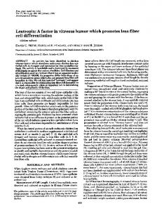
3 Image Segmentation As a precursor to feature extraction and the computation of spectral signatures for cells, segmentation of cells is required. Automatic cell segmentation is one of the most interesting segmentation problems due both to the complex nature of the cell tissues and to problems inherent to microscopy. Cytological spectral images share the following characteristics: • Poor contrast, i.e., cell gray levels may be close to that of background; • Many cluttered cells in a single view. A high number of occluding cells make image segmentation difficult; • Low quality. Traditional staining techniques introduce a lot of inhomogeneity into the images, where not all of the parts of the same tissue or cells are equally stained. • The grayscale intensity of cells vary with changing excitation wavelength. Figure 1 shows a subset of the spectral image (400nm, 500nm, 600nm, and 700nm) of a Papanicolaou stained cytological specimen where in the characteristic problems are clearly evident.

619

We employ a three-phase approach to segmenting cells in multispectral cytological images. This method is similar to the approach proposed in [4] which uses a two-phase approach for segment cells in immunostained images. We use blind deconvolution approach to identify a lower dimensional space that can be used to represent the spectral image for the purpose of segmentation. An unsupervised clustering approach coupled with cluster merging based on a fitness function is used in the second phase to obtain a first approximation of the cells location. A joint segmentation-classification approach incorporating ellipse as a shape model is used in the third phase to detect the final cell contour. Specifically, the first phase formulation is based on the use of principal components analysis followed by representativebased clustering coupled with cluster merging using proximity graphs in the second phase. Third phase formulation is based on the Level Set approach proposed by Osher and Sethian [5] coupled with a feature-based classification model and the elliptical shape prior.

3.1 Principal Component Analysis The principal component analysis or Karhunen-Loeve transform is a mathematical way of determining the linear transformation of a sample of points in Ndimensional space which exhibits the properties of the sample most clearly along the coordinate axes. Along the new axes the sample variances are extremes (maxima and minima), and uncorrelated. In addition to being able to determine the linear relationship between transformed dimensions of the data, using a cutoff on the spread along each axis, a sample may be reduced in its dimensionality [6]. In our case, we transform the spectral image, which has 31 values for each pixel, into a 3 dimensional value. We chose the first three principal components to represent the lower dimensional space and map them to an RGB image for visualization. The transformed image of the spectral image of figure 1 is shown in figure 2.

3.2 Clustering and Cell Localization

Figure 1: Four channels of a spectral image of a stained cytological smear.

The objective of the second phase analysis is to find a set of locations corresponding to the cells of interest based on the PCA transformed image. We utilize the K-Means clustering algorithm that hierarchically splits the representative color space containing colors from the cells and background regions. One of the limitations of unsupervised approaches like K-Means is the inability to predict the true number of clusters as well as the lack of arbitrary cluster shape representation. We address this problem based on post-

Proceedings of the 11th WSEAS International Conference on COMPUTERS, Agios Nikolaos, Crete Island, Greece, July 26-28, 2007

620

and Vese proposed piecewise constant active contour model [9] based on Mumford-Shah segmentation model [8], given by ∂φ(x, y) ∂t

= δǫ (φ(x, y))[νκ(φ(x, y))

(1)

−(I(x, y) − µ1 )2 + (I(x, y) − µ2 )2 ],

Figure 2: PCA transformed image of the cytological smear using the first three principal components of the spectral image. processing of the realized clusters, leading to a merge criteria to realize the final localization of cells. We utilize a post-processing technique that is similar to agglomerative hierarchical clustering in that we iteratively merge two candidates. However, it differs from a hierarchical clustering algorithm in that it merges neighboring clusters that enhance a given fitness function the most, and not necessarily merge clusters that are closest to each other. A fitness function is used that utilizes the principles of cohesion and separation [7]. The fitness function is Q(x) = Separation(x)δ /Cohesion(x)(2−δ) where, Separation(x) is defined as the ratio of total inter-cluster distances across all clusters to the inter-cluster distance of the cluster of interest, and Cohesion(x) is the ratio of the total intra-cluster distances across all clusters to the intra-cluster distance of the cluster of interest. The distances are measured as the L2-norm between a point in the cluster and the cluster center. In general, separation measures how well-separated a cluster is from other clusters while cohesion measures the tightness of a cluster. Hence, δ weighs the importance of distinct clusters to cluster compactness. The final clustering results in the optimal separation of cells and background. All pixels labeled as cells are separated into a new image and a blob coloring operation performed to count the total number of regions. Each region is than isolated as a new image for the next stage in segmentation.

3.3 Variational Segmentation Model The Mumford-Shah model [8] has been regarded as a general model within variational segmentation methods. According to Mumford-Shah′ s conjecture, the image segmentation is a variational problem of finding an optimal piecewise-smooth approximation f (x, y) of the given scalar image I(x, y) and a set of boundaries C, such that the approximation f (x, y) varies smoothly within the connected components of the subsets excluding the boundaries Ω\C. Chan

where δǫ (.) denotes the regularized form of Dirac delta function, and {µ1 , µ2 } denotes the mean of the image intensity I measured at the inside and the outside of the contours. Mumford and Shah proposed to solve the variational segmentation problem by minimizing the following global energy function: E(f, C) ≡

Z

|I(x, y) − f (x, y)|2 dxdy

(2)

Ω

+µ

Z

|∇f (x, y)|2 dxdy + ν|C|

Ω\C

The variational boundaries C have the role of approximating the edges of I(x, y) by smoothing f (x, y) only on Ω\C. The minimization of the global energy function approximates the image I(x, y) with f (x, y), smoothes f (x, y), and reduces the length of boundaries |C|. The global energy function given in equation 2 for all regions can be generalized by: E(f, C) ≡

XZ

Ωi

i

+µ

ei (x, y)dxdy

Z

Ωi \C

(3)

|∇fi (x, y)|2 dxdy + ν|C|,

where the objective function ei (x, y) determines the condition of region-based segmentation for each subset Ωi for the piecewise-constant contours shown in equation 1. Our goal here is to extend the energy functional 3 in order to force the level set to segment only the regions of interest, namely the cells constrained by specific image features and a known parametric shape. This is done in general by modifying the objective function ei (x, y) and adding a term Eshape to the global energy function that measures how well the level set represents the cell. The modified global energy functional is given by: E(f, C, Θ) ≡

X i

β

Z

Ωi

Eshape + µ

Z

α

Z

Ωi

Ωi \C

ei (x, y)dxdy + (4)

|∇fi (x, y)|2 dxdy,

Within this formulation, the smoothness constraint is automatically ensured and therefore not needed from the original Mumford-Shah model.

Proceedings of the 11th WSEAS International Conference on COMPUTERS, Agios Nikolaos, Crete Island, Greece, July 26-28, 2007

Let the (vector-valued) image intensity I be a multidimensional random variable given by I ∈ ℜB where B denotes the dimension of the image intensity I, which is also equivalent to the number of features extracted from the image I(x, y). We propose an objective function to measure how much an image pixel is likely to be an element of a subset using a probability density function (PDF) estimated from training samples. The objective function is given by ei (x, y) ≡ − log(pi (I(x, y)+P (Ωi )), ∀(x, y) ∈ Ω, ∀i, (5) where pi (I) : ℜB → ℜ denotes the multivariate conditional PDF of a vector-valued image intensity I on the condition that the image pixel I(x, y) is an element of the subset Ωi , and P (Ωi ) denotes the a priori probability of the subset Ωi . Based on the objective function of equation 5, minimizing the the first term of energy E in function 4 is equivalent to maximizing the log a posteriori probability given by pi (I(x, y))+P (Ωi ) for each subset Ωi . The computation of posterior probability is based in the use of Bayesian classification scheme as detailed in [10]. The second term Eshape is based on knowing that most human cells have elliptical shaped boundaries. To impose such a priori knowledge, we use the implicit form of the ellipse equation to describe the cell boundary given as: [(x − x0 ) cos θ + (y − y0 ) sin θ]2 a2 [(x − x0 ) sin θ + (y − y0 ) cos θ]2 b2

+

(6)

= 1

The segmentation according to an ellipse then is equivalent to the recovery of five parameters, where the space to be optimized is given by Θ = [a, b, θ, x0 , y0 ] where (x0 , y0 ) denotes the center of the ellipse, θ denotes the orientation of the ellipse, and a, b denote the major and minor axis of the ellipse, respectively. Segmentation based on explicit incorporation of cell classification and its shape representation is now equivalent to deforming an ellipse according to Θ so it is attracted to the desired image classification. The global energy function of the level set contour model and the associated Euler-Lagrange equation obtained by minimizing the global energy function E with respect to φ = φ1 , . . . , φj , . . . , φJ can be given by ∂φj (x, y) = δǫ (φ(x, y))[−µ − (7) ∂t m−1 X

α(

i=0

Pi,cell (I(x, y)) −

m−1 X i=o

Pi,bckg (I(x, y))) −

m−1 X

β(

i=0

(1 −

621

q

(A/a)2 + (B/b)2 ))]

where, A = (xi − x0 ) cos θ + (yi − y0 ) sin θ and B = −(xi − x0 ) sin θ + (yi − y0 ) cos θ. The solution to the Euler-Lagrange is implemented using gradient descent where the parameters for the ellipse, Θ, are solved at each iteration of the level set evolution [11, 4]. Figure 3 shows three representative localized regions and the corresponding cell segmentation obtained based on segmentation approach. A total of 40

Figure 3: Segmentation of three cells within the corresponding localized regions. The top row shows the localized regions and the contour initialization. The bottom row shows the final contour for each of the regions. spectral images were segmented to evaluate the approach. This resulted in cell segmentation accuracy rate of 92.1% with a missed segmentation rate of 4.3% and a false segmentation rate of 2.7%. The segmentation errors encountered were primarily due to the failure of the localization stage in identifying the correct region of interest.

4 Feature Extraction and Classifiers To evaluate the utility of spectral imaging, we performed classification studies for automated identification of the different cell types, specifically for the automated differentiation between red blood cells (RBC), white blood cells (WBC), squamous epithelial cells (SQP), and non-squamous epithelial cells (NSQP). A total of 51 clinical samples were imaged. The number of samples and the number of cells processed for each cell type are listed below in table 1. Each spectral image set was PCA transformed and cells segmented. A binary mask was generated for each segmented cell to extract the corresponding area from each of the 31 spectral images. Gray level image intensities were used to determine the portion of light transmitted by each cell across the exciting spectra. The radiation transmitted by the cell was measured as the integrated intensity of the cell divided by the area of the cell. The intensity of the incident light

Proceedings of the 11th WSEAS International Conference on COMPUTERS, Agios Nikolaos, Crete Island, Greece, July 26-28, 2007

Type Samples Cells

RBC 7 154

WBC 16 151

SQP 13 72

NSQP 15 49

Features MORPH (38) SPEC+MORPH (40)

NBC 68.8% 79.9%

Classifier BN 66.5% 81.1%

622

MLP 61.2% 85.2%

Table 1: Number of samples and cells processed. was estimated by measuring the average intensity of the background (i.e. the surrounding media around the cell). The background area was chosen as an extension around the cell area, three pixels away and five pixels thick. The transmission factor was T = It /Ii , where It is the intensity of the light transmitted by the cell and Ii is the intensity of incident light. Using the Beer-Lambert law [12], the absorption parameter is calculated by Abs = log(1/T ). This computation was performed for each of the 31 wavelengths, resulting in 31 spectral measures for each cell (spectral profile). In addition, 71 morphological features were also computed. These features ranged from standard descriptors such as area, size, perimeter, to textural and fractal features [13]. These measure are computed using only the 550 nm wavelength image. A total of 102 features were computed for each cell, comprised of 31 absorption parameter factor values, and 71 morphological features, including image; size, mean, standard deviation, contrast, and cell; width, height, perimeter, area, shape factor1, shape factor2, mean, standard deviation, contrast, fractal dimension1, fractal dimension2, average entropy, entropy homogeneity, roughness, low entropy emphasis, high entropy emphasis, low graylevel entropy emphasis, high graylevel entropy emphasis, concavity and 48 statistical geometric features. In order to design optimal classifiers, a first analysis was performed to select a smaller subset of morphological and spectral features. We performed feature selection for the spectral and morphological measures separately. This was based on an exhaustive search of all combinations of the features, with the criteria of selection based on maximizing the correlation of the chosen features to the cell classes. This resulted in a smaller set of features comprising 2 spectral measures and 38 morphological features. The spectral features chosen included the normalized transmission factor for 400nm and 700nm, while the morphological features selected included image; size, mean, standard deviation, contrast, and particle; width, perimeter, area, shape factor1, shape factor2, mean, contrast, fractal dimension1, fractal dimension2, average entropy, entropy homogeneity, high graylevel entropy emphasis, concavity and 20 statistical geometric features. Thus a total of 40 features, of the original 102, were used.

Table 2: Classification accuracy for three classifiers without bagging. Features MORPH (38) SPEC+MORPH (40)

NBC 70.2% 85.2%

Classifier BN 78.7% 81.5%

MLP 73.8% 88.0%

Table 3: Classification accuracy for three classifiers with bagging. To evaluate the merit of the extracted features, we used six different classification methods. They were based on a Na¨ıve Bayes classifier (NBC), a Bayesian Network (BN), and a Multilayer Perceptron (MLP) neural network [14]. We also tested a metaclassification approach based on bagging [15]. Bagging, a common approach used to improve the performance of a classifier, uses multiple classifiers that vote to generate a final decision. We created a baggingbased classifier for each of the classifiers. We further wanted to compare the benefit of using the spectral features versus morphological features. We ran the classifiers using only morphological features, and then using a combined set of spectral and morphological features. All performance analysis was based on the leave-one-out cross validation approach. The best classification performance resulted from using MLP with bagging. An overall increase of 15% in classification accuracy is seen with the use of the combination of spectral (SPEC) and morphological features (MORPH). Tables 2 and 3 show the correct classification rates for the three classifiers, with and without bagging, respectively. We chose the Bagging MLP, as it was the classifier with the best classification rate. In addition, to understand the behavior of the classifier, we computed the sensitivity and positive predictive value (PPV) for each of the individual classes. The sensitivity is computed as the percentage of the cells that actually belong to one category that are assigned to that category. Positive predictive value is computed as the percentage of the cells that are assigned to one category that actually belong to that category. Tables 4 and 5 show the sensitivity and PPV for the Bagging MLP, compared across classification based on morphological features and on the combined spectral and

Proceedings of the 11th WSEAS International Conference on COMPUTERS, Agios Nikolaos, Crete Island, Greece, July 26-28, 2007

Type MORPH SPEC & MORPH

RBC 88.3 87.7

WBC 88.1 88.1

SQP 93.5 93.5

NSQP 53.8 61.5

Table 4: Sensitivity (%) of the Bagging MLP Classifier. Type RBC WBC SQP NSQP MORPH 97.3 97.2 99.0 98.8 SPEC & MORPH 97.7 97.7 98.8 99.2 Table 5: Positive Predictive Value (%) of the Bagging MLP Classifier. morphological features. As seen, the spectral features generally improve classification of cell subtypes, with increased sensitivity, and reduced false positive rates. These results prove the feasibility of using spectral data for improved automated cell differentiation.

5 Summary and Conclusions We have presented a multispectral microscopy system and shown its benefit to the problem of cell differentiation. Algorithms for automated cell segmentation, spectral and morphological feature extraction, and the design and evaluation of classifiers are discussed. While conventional practices in microscopy rely on the analysis of grey scale or RGB color images, presented system uses thirty one spectral bands for analysis. Results of the developed system are presented and classification performance is compared to the case where multispectral information is not taken into consideration. Results show that the developed system and the use of multispectral information along with morphometric information extracted from spectral images can significantly improve the classification performance and can aid in the process of identifying and differentiating various cell types present in a cytological sample. Acknowledgements: The data collection and analysis was supported by the NIH SBIR Grant (grant No. 1 R43 DK67750). References:

623

Imaging, Chemical Analysis Series. John Wiley & Sons, New York, 1996. [3] S. Shah, J. Thigpen, F. Merchant, and K. Castleman, “Photometric calibration for automated multispectral imaging of biological samples,” in Proc. of Workshop on Microscopic Image Analysis with Applications in Biology (in conjunction with MICCAI, Copenhagen), D.N. Metaxas, R.T. Whitaker, J. Rittscher, and T.B. Sebastian, Eds., 2006, pp. 27–33. [4] S. Shah, “Automatic cell segmentation using a shapeclassification model,” in Proceedings of IAPR Conference on Machine Vision Applications, 2007, pp. –. [5] S. Osher and J. Sethian, “Fronts propagating with curvature dependent speed: Algorithms based on Hamilton-Jacobi formulations,” Journal of Computationl Physics, pp. 12–49, 1988. [6] C. M. Bishop, Neural Networks for Pattern Recognition, Oxford University Press, New York, 1995. [7] J. Choo, R. Jiamthapthaksin, C. Chen, O. Celepcikay, C. Giusti, and C. Eick, “Mosaic: A proximity graph approach to agglomerative clustering,” in Proc. 9th International Conference on Data Warehousing and Knowledge Discovery (DaWaK), 2007. [8] D. Mumford and J. Shah, “Optimal approximation by piecewise smooth functions and associated variational problems,” Communication Pure and Applied Mathematics, p. 577, 1989. [9] L. Vese and T. Chan, “A multiphase level set framework for image segmentation using the Mumford and Shah model,” International Journal of Computer Vision, , no. 3, pp. 271–293, 2002. [10] S. Shah, “Segmenting biological particles in multispectral microscopy images,” in Proceedings of IEEE Workshop on Application of Computer Vision. 2007, pp. 44–49, IEEE Computer Society. [11] Y. Tang, X. Li, A. von Freyberg, and G. Goch, “Automatic segmentation of the papilla in a fundus image based on the c-v model and a shape restraint,” in Proc. of International Conference on Pattern Recognition, 2006, pp. I: 183–186. [12] R. L. Ornberg, M. Woerner, and D. A. Edwards, “Analysis of stained objects in histopathological sections by spectral imaging and differential absorption,” J. Histochem. Cytochem., vol. 47, no. 10, pp. 1307– 1313, 1999.

[1] H.S. Wu, J. Barba, and J. Gil, “A parametric fitting algorithm for segmentation of cell images,” IEEE Trans Biomed Eng, vol. 45, pp. 400–407, 1998.

[13] K. R. Castleman, Digital Image Processing, Prentice Hall, 1998.

[2] Y. Garini, N. Katzir, D. Cabib, R. Buckwald, D. Soenksen, and Z. Malik, Fluorescence Imaging Spectroscopy and Microscopy, chapter Spectral Bio-

[15] R. O. Duda, P. E. Hart, and D. G. Stork, Pattern Classification, Wiley, 2001.

[14] T. Mitchell, Machine Learning, McGraw Hill, 1997.