Automated, Contract-based User Testing of Commercial - CiteSeerX

Carleton University, TR SCE-05-16

October 2005

Automated, Contract-based User Testing of CommercialOff-The-Shelf Components Lionel, C. Briand ‡,§

Yvan Labiche ‡

‡

Carleton University Department of Systems and Computer Engineering 1125 Colonel By Drive Ottawa, ON K1S5B6, Canada {briand, labiche, msowka}@sce.carleton.ca

Michal Sówka ‡ §

Simula Research Laboratory Department of Software Engineering Martin Linges v 17, Fornebu P.O.Box. 134, 1325 Lysaker, Norway [email protected]

ABSTRACT Commercial-off-the-Shelf (COTS) components provide a means to construct software (component-based) systems in reduced time and cost. In a COTS component software market there exist component vendors (original developers of the component) and component users (developers of the component-based systems). The former provide the component to the user without source code or design documentation, and as a result it is difficult for the latter to adequately test the component when deployed in their system. In this report we propose a framework that clarifies the roles and responsibilities of both parties so that the user can adequately test the component in a deployment environment and the vendor does not need to release proprietary details. Then, based on this framework we combine and adapt two specification-based testing techniques and describe (and implement) a method for the automated generation of adequate test sets. An evaluation of our approach on a case study demonstrates that it is possible to automatically generate cost effective test sequences and that these test sequences are effective at detecting complex errors.

KEYWORDS COTS, Component, UML, Adequacy Criteria

1


October 2005

1 INTRODUCTION The concept of software components, software modules, or more generally software reuse, is not new and dates back to the late 1970s. The structure-oriented software development methodology of the time often limited the reuse of the software modules to within the scope of a project. More recently, object-oriented development methodologies have facilitated packaging of sub-systems into software modules for reuse across development teams and projects. Modern software models such as ActiveX, CORBA, and Enterprise JavaBeans (EJB) take a further step in promoting code reuse. A software component, adopting the definition provided in [36], is a “unit of composition with contractually specified interfaces and context dependencies only. A software component can be deployed independently and is subject to composition by third parties.” Composition is the assembly of one or more software components into composite software systems. Contractually specified interfaces are either of the two following types: provides representing the functionality that the component provides; or requires representing the functionality that the component requires (e.g., from other components). By specifying strict interfaces through which they are deployed and exercised, modern component models1 allow component reuse across organizations and create a Commercial-off-the-Shelf (COTS) component market which consists of component vendors and component users. Component users purchase the vendors’ components for use in their component-based software systems deployed on a specific deployment platform. The deployment platform typically consists of computer hardware and network, operating system, system services (e.g., email address lookup), and a component container providing (among other things) the interfaces required for component deployment. Component containers are implemented strictly according to the specification of a particular component model (e.g., EJB). Component-based software engineering has many advantages [36]: the most obvious ones are reusability and reduced costs. But they also pose new challenges to component users that are 1

In this report, unless accompanied by contractually specified (possibly standard-based) provides and requires interfaces, class packages and libraries are not considered software components. 2


October 2005

non-issues in traditional software development practices [20]. One of these challenges is the evaluation (verification and validation) of a component by the user on a specific deployment platform, for instance by means of testing techniques. Four main reasons are: -

Heterogeneity of deployment platforms: The user may not necessarily use a platform on which the component has been evaluated by the vendor.

-

Limited Test model: Because no source code or design information is usually provided, the information to develop a test model is often limited to textual documentation and an API. Controllability and observability are then limited [7].

-

Difficult definition of testing adequacy criteria: Although component interfaces are described according to specific component models, they often do not provide much information that can be used to define functional testing adequacy criteria. The component user has to mostly rely on the textual documentation of the component. For instance, the often used adequacy criteria all-method and all-exception have been shown to be insufficient [21].

-

Generality of components: Components are often designed for broad applicability, whereas users often require only a subset of the provided functionalities. Users cannot afford to test the entire component and need techniques to select component partitions to be tested. This need has been illustrated for instance by the formal component model provided in [33].

The main contributions of our work include: (i) The definition of test adequacy criteria in a context where no source code and design information is available (Section 4); (ii) An automation framework, including an algorithm for the construction of an adequate but minimal set of test sequences for those criteria (Section 5). The report starts with a review of related work (Section 2) and discusses how the component vendor could facilitate deployment testing activities performed by the user without revealing proprietary details (Section 3). Our test technique is then detailed in Sections 4 and 5. It is evaluated in Section 6 on an actual component and conclusions are drawn in Section 7.

3


October 2005

2 RELATED WORK A variety of functional testing techniques can be considered for component testing. First of all, some that rely only on a textual documentation come to mind (e.g., Category Partition [31]). However, we describe in Sections 2.1 to 2.3 three other techniques that can be used by the component user and are amenable to the automatic generation of adequate test sets. Section 2.4 discusses a strategy that component vendors can use to conveniently provide (testing) artifacts to the component user.

2.1 CSPE Constraint-Based Testing Constraints on Succeeding and Preceding Events (CSPE) is a testing technique originally used for the functional testing of concurrent programs [10], and more recently used for class unit testing [14]. Following the CSPE technique, CSPE constraints on sequences of invocation of pairs of methods are first derived from the specification. We denote them as 3-tuples (preceding method, succeeding method, constraint predicate) indicating that a call to the succeeding method can be performed after a call to the preceding method when the constraint predicate is true. CSPE constraints, and more specifically constraint predicates, can be derived from method preconditions and postconditions. The postcondition of the preceding method either implies, contradicts, or partially implies the precondition of the succeeding method, resulting in four types of constraints: Always Valid, Never Valid, Possibly Valid, and Possibly Invalid. In the first two cases, the 3-tuple predicate is always true or always false. The latter two are complementary: Invoking the succeeding method immediately after the preceding method is valid (resp. invalid) only when a specific predicate is true (resp. false). A Possibly Valid constraint occurs when the postcondition of the preceding method does not imply the precondition of the succeeding method, but the conjunction of the preceding method’s postcondition and the 3-tuple predicate implies the precondition of the succeeding method. Test cases based on CSPE constraints are constructed by concatenating constraints together. Constraints are concatenated such that the succeeding method of the first constraints matches the preceding method of the second constraints. Consecutive constraints are concatenated in a similar manner until all constraints have been covered. Since a test case has to begin with a

4


October 2005

constraint void of a preceding method, a method labeled # is used to represent the start of a test case [10]: for instance, constraint (#, m1, true) indicates that component interface method m1 can always be executed at the start of the test case. In the context of component testing, this also corresponds to component instantiation. With this in mind, a component of n interface methods, then has n2+n constraints to be considered: the first term accounts for constraints of ordered pairs of methods, whereas the second accounts for constraints with preceding method #. CSPE constraints can be used to generate test cases according to four CSPE constraint coverage criteria [14]. Always Valid Coverage (A) requires that all Always Valid constraints be covered at least once. Always/Possibly Valid Coverage (AP) includes both Always Valid and Possibly Valid constraints. Never Valid/Possibly Invalid Coverage (NP) requires that all Never Valid and Possibly Invalid constraints be covered at least once. Finally, Always/Possibly Valid/Never Valid/Possibly Invalid Coverage (ANP) requires that all constraints be covered at least once. It is also possible to add a Never Valid Coverage criterion (N) that requires covering only the Never Valid constraints. It is important to note that Possibly Valid and Possibly Invalid constraints conceptually represent only one constraint since the predicates involved in the latter are the negations of predicates involved in the former. Automatically constructing adequate test sets for these criteria is possible, as suggested in [14], by following the heuristic approach presented in [23]: It consists in building a tree where nodes are the CSPE constraints to be covered according to the selected criterion and arcs represent the concatenation of the CSPE constraints into test sequences: concatenating constraints (m1, m2, true) and (m2, m3, true) for instance amounts to executing methods m1, m2 and m3 in

sequence. Tree paths then form an adequate test for the selected criterion. The tree is grown breadth first, appending method sequence constraints from the set of constraints to be covered. Growth is terminated once all of the constraints have been covered in the tree, such that each constraint is covered at least once. The construction of the tree path also stops when a Never Valid or Possibly Invalid constraint is reached as this would result in an exception being thrown, reporting the incorrect use of the succeeding method. The tree is then pruned to reduce its size while still satisfying the criterion, resulting (because of the breadth first construction) in a test set composed of a large number of short test cases (tree paths).

5


October 2005

2.2 Testing Logical Expressions A number of coverage criteria have been defined for logical expressions. We use them when defining our test criteria in Section 4.2 in cases where complex predicates are involved in CSPE constraints: predicate coverage, combinatorial coverage, implicant coverage, prime implicant coverage [2, 7]. Predicate Coverage (PC) requires that the selected tuples of predicate clauses test the predicate twice, once such that it evaluates to true and once for false. Combinatorial Coverage (CoC) requires that all possible combinations of clauses’ truth values be exercised2. Implicant Coverage (IC) requires that the selected tuples test the predicate such that each implicant is true at least once, where implicants are disjuncts in the Disjunctive Normal Form of the predicate and its negation. Prime Implicant Coverage (PIC) requires that the selected tuples test the predicate such that, for the predicate and its negation, each implicant is set to true while all other implicants are false. The reader interested in more formal definitions is refered to [2, 7]. PC is a weak criterion (only two test cases are required), and CoC is an exhaustive criterion. The other two criteria, IC and PIC, are intermediate criteria in terms of cost (i.e., number of test cases), PIC being more costly than IC. Additionally, PIC has been shown to be very cost effective [39].

2.3 Statechart-Based Component Testing Following the strategy reported in [5], components used in a component-based systems are assumed to be described with state machines. Those state machines are used to build a control flow graph of the overall behavior of all the components. The component user can then apply traditional control and data flow testing techniques for devising test cases. It is worth mentioning that the level of details in the components’ state machines can have an important impact on what the user can achieve. If the state based behaviors are specified with too much detail, the control flow graph will likely be very large and difficult to use for devising test

2

A clause is a Boolean variable, the negation of a Boolean variable, or, in the context of OCL, an OCL constraint, i.e., an OCL expression that evaluates to true or false, without logical connectors. 6


October 2005

cases (structural testing techniques, for instance, based on control flow graphs are not known to scale up very well). Note also that too many details would likely reveal vendor proprietary information, which contradicts one of our working hypotheses. If on the other hand the behavior is provided at a high level of abstraction, state machines will likely not be very useful to the user to devise interesting test cases. If the component is large and complex, the statechart is in any case likely to be unwieldy and difficult to use, especially for users having no detailed design information about the component. As a result of the above issues, this report will not make use of state machine representations to test the components’ behavior.

2.4 Component Metadata to Support Testing A standard was suggested in [11, 30] as an extensible way for the component vendor to provide varying kinds of artifacts to be used by the component user, which are referred to as metadata. It is argued that any software engineering artifact used in component based development (e.g., testing artifacts) can be a metadatum for a given component as long as 1) the component vendor is involved in its production, 2) it is packaged with the component in a standard way, and 3) it can be processed by automated development tools and environments. Metadata describe either static (they never change) or dynamic (they may change at runtime) aspects of the component. Examples of static metadata include deployment information, textual descriptions, and version information. Structural coverage achieved when executing component methods is an example of dynamic metadata [30].

3 OVERVIEW Figure 1 is a UML activity diagram depicting an overview of our COTS component testing strategy. It illustrates the roles and responsibilities of the component vendor and user (the two horizontal swim lanes of the diagram) in terms of the information that is generated and used for component testing purposes. Recall that in a UML activity diagram [19] rounded boxes denote activities, squares boxes denote objects (data, documents, or artifacts in our case), plain arrows denote control flow, and dashed arrows dependencies between activities and objects.

7


October 2005

More specifically, the vendor (upper swim lane) defines CSPE constraints for the component interface methods (activity 1), for instance from design documents of the component. The vendor is also responsible for providing CSPE probes (activity 2), that is built-in methods that the user can use to increase controllability and observability during component testing (e.g., to put the component in a specific state). On the other hand (lower swim lane), the first task of the user (activity 3) is to identify the component functionalities that are required by the component-based system being developed (e.g., from the design documentation): the user does not necessarily need to test the whole component. Depending on constraints such as budget, the user also selects a CSPE-based testing criterion among the ones we define in Section 4.2 (activity 4). Once activities 1 to 4 have been completed (the vertical bar denotes a join), the user can proceed with the generation of an adequate test set (automated as described in Section 5), given the component functionalities under test and the selected criterion (activity 5). Then the test scaffolding (drivers, stubs, oracles) can be produced and the test cases executed (activities 6 to 7). COTS component API documentation

CSPE constraints

1: Generate CSPE Constraints

2: Implement CSPE Probes

CSPE probes

control flow data flow

Component Vendor Component User

3: Specify Targeted Functionality

4: Specify Criteria

COTScomponent-based system design

CSPE criteria

5: Generate Test Sequences

6: Generate Test Scaffolding

7: Execute Test Suite

targeted functionalities

test sequences

test scaffolding

Figure 1. COTS Component Testing Strategy Overview (UML Activity Diagram) Applying the approach proposed in Section 4, which is based on CSPE constraints, requires that some component metadata be available. First, to derive test sequences, we will need the

8


October 2005

component to provide us with the CSPE constraints themselves (static metadata). Note that clauses in predicates should not and need not be provided in any detail: symbols can be used as placeholders for clauses, as described in section 4.1. That way, no (proprietary) details are provided to the user who can still use CSPE constraints to generate test. (Note however that in the rest of the report we will use complete clauses instead of symbols to ease comprehension.) Required dynamic metadata include whether a method pre or post-condition holds at run-time and is used as an oracle during the execution of test suites. Accessing such dynamic metadata is performed through calls to specific methods that need to appear in the component interface, referred to as Built-In Test (BIT) support [7] or probes. Probes are also required to increase controllability, i.e., to make sure clauses are true when needed. Note that BIT support is a vendor technique widely discussed (e.g., many chapters in [6] describe possible approaches). They however all assume that test cases be defined by the vendor and directly embedded into the component, thus preventing any tailoring of the testing activity by the user, besides enabling auto-testing. Figure 1 captures the framework to be used when reasoning on component vendor and user responsibilities to ease component testing in the context of a particular component deployment. It’s worth noting that this framework, although described in the specific context of CSPE-based testing, is generic enough and can be used with other component-oriented testing techniques. Although vendors and users may consider another testing technique, the following activities are still required: the vendor must provide testing information and built-in test support (activities 1 and 2); the user must be able to target a specific subset of the component functionalities and use the information provided by the vendor to generate test cases from testing criteria and execute them (activities 3 through 7). Providing strategies for all these activities is a long term effort and this report is mostly concerned with activities 3, 4, and 5. Existing approaches can be considered to help automate activities 6 and 7 [32].

9


October 2005

4 COTS COMPONENT TEST STRATEGY Our COTS component test strategy is described by first revisiting a number of additional issues regarding CSPE constraints (Section 4.1). We then provide definitions for our CSPE-based test adequacy criteria (Section 4.2) which combines CSPE constraints and the testing of logical expressions. Section 0 shows how the user can identify the parts of the component to be tested. A simple example illustrates those concepts in Section 4.4.

4.1 Revisiting CSPE Constraints Recall that a CSPE constraint is composed of three parts represented in a 3-tuple (m1, m2, p): m1 is the preceding method, m2 is the succeeding method, and p is the constraints predicate. The constraint predicate implies the validity of the constraint, i.e., it evaluates to either true or false and this specifies whether the constraint is valid or invalid, respectively. The constraint predicate p is expressed in a Boolean expression. For Always Valid constraints the predicate p is a

Boolean literal true, for Never Valid constraints it is a Boolean literal false, and for Possibly Valid and Possibly Invalid constraints it is an actual Boolean expression composed of one or more Boolean variables. Note that these CSPE constraints, including constraint predicates, can be derived from a number of different sources such as: contracts in OCL [38] (or any formal language), sequence diagrams, statecharts, or even partially from textual documentation of how the component is to be used. Therefore, CSPE-based testing can be used in different contexts and in a variety of situations. The use of method preconditions and postconditions was mentioned in Section 2.1, and in fact, for our case studies such method contracts were used to derive CSPE constraints and constraint predicates. Additionally, those contracts are written in OCL. In other words, for each constraint (m1, m2, p), p is derived such that the OCL postcondition of m1 in conjunction with p implies the OCL precondition of m2. OCL expressions require a context, that is the model element for which the OCL expression is defined, which is in genEral either a class or an method [38]. Since predicate p is derived from m1’s postcondition and m2’s precondition, both m1 and m2 are candidates for the context of p. On the other hand, since p indicates what is not ensured by m1 but

10


October 2005

required by m2, p may contain parts of m2’s precondition (e.g., p may indicate that some parameters of m2 have specific values). The context of p is thus succeeding method m2. OCL pre and postconditions, and thus constraint predicates may reveal too many details about the component, suggesting for instance its design (e.g., parts of its class diagram), which can be considered proprietary information by the component vendor. Indeed, a constraint predicate may contain an OCL expression like self->MyClass.attr=1, suggesting that the component contains a class named MyClass with an attribute of type integer named attr. (Class MyClass may not be publicly available through the component interface.) The issue of deciding what information the component vendor has to provide in constraint predicates is out of the scope of this report. We however provide here some directions for future work. One way to address this issue is to study different levels of details for OCL expressions such as those reported in [40]. Another solution is to use symbols as placeholders for clauses in OCL constraint predicates. That way, no (proprietary) details are provided to the user who can still use CSPE constraints to generate tests. Specifically, if a detailed version of a constraint predicate reads self.MyClass->attr=1 or self.a=10, which is considered to reveal too many internal details by the component vendor, the component vendor can simply provide constraint A or B to the component user. The user is still able to use predicate testing criteria. The user

simply requires mechanisms, provided by the vendor in the component interface, to ensure (without knowing the details) that clauses A or B are satisfied when executing a test case. The component vendor can for example provide methods isA() and isB(), both returning Boolean values, to check whether clauses A and B are true. Additionally, the vendor can provide methods setA() and setB() to allow the user to set the value of the clauses. Alternatively, when setting

the value of a clause turns out to be difficult with one method call, the component vendor can provide a sequence of public method executions that result in A or B being true.

4.2 CSPE-Based Test Adequacy Criteria Because the predicates involved in CSPE constraints can be complex, and because we need to make sure that testing exercises the various situations under which two methods can execute in a sequence, CSPE-based testing criteria need to account for both the constraint type and the logic of the constraint predicate. We thus combine CSPE criteria (Section 2.1) and logical expression 11


October 2005

testing criteria (Section 2.2), and define a total of 14 CSPE-based test adequacy criteria as reported in Table 1. We therefore have five ways to account for constraint types (first two columns in Table 1): A, AP, N, NP, and ANP. Then, for AP, NP, and ANP, which involve Possibly Valid and Possibly Invalid constraints, we also account for varying ways of exercising predicates, using criteria PC, IC, PIC, and CoC (third column). PC and CoC provide two extreme situations whereas IC and PIC are intermediate in terms of cost-effectiveness (where, again, PIC has been found to have a good cost-effectiveness in [39]). Table 1 (last column) shows the acronyms for our 14 CSPEbased test adequacy criteria. Table 1. Definition of CSPE-based Test Adequacy Criteria Definition The criterion requires that every Always Valid constraint be covered at least once. The criteria require that every Always Valid constraint be covered at least once, and that every Possibly Valid constraint be covered according to one of the predicate criteria Predicate Coverage (PC), Implicant Coverage (IC), Prime Implicant Coverage (PIC), Combinatorial Coverage (CoC). Only solutions to the selected predicate criterion leading to a truth value of the predicate are selected. The criterion requires that every Never Valid constraint be covered at least once. The criteria require that every Never Valid constraint be covered at least once, and that every Possibly Valid constraint be covered according to one of the predicate criteria Predicate Coverage (PC), Implicant Coverage (IC), Prime Implicant Coverage (PIC), Combinatorial Coverage (CoC). Only solutions to the selected predicate criterion leading to a false value of the predicate are selected.

Constraint type(s)

Acronyms Predicate CSPE-based Criterion criterion

A

N/A

A

PC

AP–PC

IC

AP–IC

PIC

AP–PIC

CoC

AP–CoC

N/A

N

PC

NP–PC

IC

NP–IC

PIC

NP–PIC

CoC

NP–CoC

PC

ANP–PC

IC

ANP–IC

PIC

ANP–PIC

CoC

ANP–CoC

AP

N

NP

The criteria require that every Always Valid and every Never Valid constraints be covered at least once, and that every Possibly Valid constraint be covered according to ANP one of the predicate criteria Predicate Coverage (PC), Implicant Coverage (IC), Prime Implicant Coverage (PIC), Combinatorial Coverage (CoC).

In some cases (for constraint types AP and NP), the definitions indicate that only a subset of the test cases required by the selected logical expression testing criterion is used. The reason is that these CSPE-based criteria exercise either true or false values of the predicate (but not both). 12


October 2005

4.3 Targeting Functionalities Recall that the component user should be able to specify which parts of the component, i.e., functionalities of the component, under test, since the component-based system being built by the user may not use all of the component’s functionalities. We have identified two complementary partitioning strategies, referred to as Required Methods, and Required Constraints. The Required Methods partitioning consists of two steps. First, the user specifies a subset of the component interface methods that are actually used. (The initialization method, labeled #, is always part of this set.) This can be done manually from the user understanding of how the component-based system uses the component, or automatically from UML sequence diagrams showing how that system interacts with the component. The second step is to select a subset of the CSPE constraints based on this subset of component interface methods. Only constraints that involve preceding and succeeding methods identified during the first step are selected. In other words, if component methods m1 and m2 appear in UML sequence diagrams, then constraints (m1, m2, p) and (m2, m1, p’) are selected.

For the Required Constraints partitioning, the user directly selects CSPE constraints to be exercised. This can be done manually or automatically too. For instance, in the latter case, if UML sequence diagrams show two interface methods m1 and m2 called always in that order, then only constraint (m1, m2, p) should be selected. Once constraints have been selected, according to either of the two partitioning strategies described above, the user can use any of the CSPE-based criteria to further select constraints.

13


October 2005

4.4 Example We illustrate the concepts introduced above with the simple Queue component example in Figure 3. Figures (a) and (b) are the component class diagram and a possible usage by a user, respectively. Figure (c) recalls the methods that appear in Figure (a) but also provides pre and postconditions in OCL for the component interface methods. Figure (d) is an excerpt of the CSPE constraints for Queue: a total of 56 constraints, including 10 Always Valid constraints, 15 Never Valid constraints, and 31 Possibly Valid constraints. (A complete list can be found in Appendix A.) The Queue component wraps and provides access to a linked list of arbitrary objects. It requires initialization before use, including setting its initial state. The component has seven interface methods: init, empty, eque, dque, top, getLock, and rlsLock. Method init initializes the component before it can be used, empty checks if the Queue is empty, eque and dque add and remove an item to the queue respectively, and top fetches the last item off the queue without removing it. The Queue component exposes two provides interfaces (Figure 2): Producer, and Consumer. Each is an interface to a subset of the seven interface methods of the component. The Producer interface is meant to be used by a client program that initializes the Queue component and enqueues to it, while the Consumer interface is meant to be use by a client program that checks for the status of the queue and de-queues from it. Some interface methods are exclusive to each of the interfaces (eque appears in Producer, whereas dque appears in Consumer), while others are accessible from both (empty, getLock, rlsLock). Producer Consumer

Queue

Producer

Consumer

+init(): void +empty(): boolean +eque(obj:Object): void +getLock(lock:Lock): void +rlsLock(lock:Lock): void

+empty(): boolean +dque(): Object +top(): Object +getLock(lock:Lock): void +rlsLock(lock:Lock): void

Figure 2. Requires and Provides interfaces for the Queue

14


October 2005

Methods getLock and rlsLock are used to get and release a synchronization lock on the Queue instance making the component thread safe in a multi-threaded environment: methods that modify the Queue component require that the Queue component be in either an unlocked state (for a single-threaded client), or that the calling thread hold the current lock (for a multi-threaded client). The constraints reported in Figure 3 (d) are devised from the component OCL contracts in Figure 3 (c). For instance, pre and post-conditions show that calling empty immediately after init is always possible (c9) whereas calling init twice is never valid (c8). Calling eque immediately after init requires that the client holds the current lock or there is no locking mechanism as specified in the two clauses of predicate p1 (c10). Selecting the Always Valid constraints for testing (A) requires exercising 10 constraints. Selecting Always Valid and Possibly Valid constraints (e.g., with AP-PC) requires exercising 41 constraints. In combination with AP, PC requires that each Possibly Valid predicate (e.g., p1) be exercised once. Variants of ANP (e.g., ANP-CoC) require exercising all 56 constraints. CoC, in combination with ANP, implies that predicate p1 (for instance) be exercised four times (four truth value combinations of the two clauses of p1). Assuming the usage of Queue specified in Figure 3 (b) and following the Required Methods partitioning strategy, constraints c10 and c22 are selected (among others). On the other hand, following the Required Constraints strategy would lead to the selection of only c10 if no sequence diagram shows eque being executed before init.

15


October 2005

Initial value is uninitialized

top():Object

Lock

-lock Lock instance is empty in case the Queue is not held in a lock

0..1 ...

getLock():void top():Object

(a) Component class diagram

(b) Example of component usage context Queue::getLock(l:Lock) pre : post: if lock@pre->isEmpty()then lock = l endif

context Queue::init() pre : state = #uninitialized post: state = #empty context Queue::empty():Boolean pre : state #uninitialized post: if state = #empty then result = true else result = false endif

context Queue::rlsLock(l:Lock) pre : lock = l post: lock->isEmpty() context Queue::dque(l:Lock):Object pre : state = #partiallyFill and (lock = l or lock->isEmpty) post: size = size@pre – 1 and result = top()@pre and if size = 0 then state = #empty else state = #partiallyFull endif

context Queue::eque(obj:Object,l:Lock) pre : state #uninitialized and (lock = l or lock->isEmpty) post: size = size@pre + 1 and top() = obj context Queue::top():Object pre : state #uninitialized state #empty post: not result->isEmpty

init():void eque(obj:Object):void

...

+init() +empty(): boolean +eque(obj: Object,lock: Lock) +dque(lock: Lock): Object +top(): Object +getLock(lock: Lock) +rlsLock(lock: Lock)

q:Queue

Component-based System

-state State 1 uninitialized empty partiallyFull

Queue

and

(c) Component methods with OCL pre and postconditions c1=(#,init,true) c2=(#,empty,false) c10=(init,eque,p1) c9=(init,empty,true) c8=(init,init,false) c13=(init,getLock,p2) c26=(eque,top,true) c11=(init,dque,false) c24=(eque,eque,p1) c30=(dque,empty,true) c22=(eque,init,false) c47=(getLock,top,p5) c37=(top,empty,true) c48=(getLock,getLock,false) c38=(top, dque, p1) c44=(getLock,empty,true) c12=(init, top, false) p1 = (lock->isEmpty or lock = l) p5 = (size 0) p2 = (lock->isEmtpy())

(d) Excerpt of CSPE constraints (with predicates) Figure 3. The Queue example

5 AUTOMATION We have automated the generation of adequate test sets for the criteria defined in Section 4.2. This involves representing constraints in a graph (Section 5.1), associating costs to arcs in the graph (Section 5.2), and devising algorithms to traverse the graph (Section 5.3).

16


October 2005

5.1 Graph Representation We decided to adopt a graph representation for constraints that have to be covered according to the selected CSPE criterion. In this graph, nodes are component interface methods (including #) and arcs represent CSPE constraints. Each Always Valid constraint c = (m1, m2, true) is modeled as an arc from node labeled m1 to node labeled m2, and the arc is labeled c. Each Never Valid constraint c = (m1, m2, false) is modeled as an arc from node labeled m1 to an error node for method m2, labeled m2 , and the arc is labeled c. There is only one way to leave an error node, which is to follow an arc from this node to node #. This arc is labeled ‘~’ and represents the re-instantiation of the component. In order to facilitate the identification of short test cases or test cases of low cost, such reinstantiation arcs are added to all the nodes in the graph. Then, during the traversal of the graph, looking for an adequate test set, those arcs can be taken if it means reducing the overall cost of the test set3. Each Possibly Valid constraint c = (m1, m2, p) leads to two different arcs because both valid and invalid outcomes might need to be exercised according to the selected criterion. Additionally, Possibly Valid constraints may have to be exercised several times according to the selected predicate criterion (e.g., CoC), for different combinations of clauses truth values. Thus, for each selected combination of clause truth values resulting in a true value for the predicate there is one arc, labeled “c [true, n]” where n is the integer value corresponding to the combination4, from node labeled m1 to node labeled m2. Similarly, for each selected Boolean variable value combination resulting in a false value of the predicate there is one arc, labeled “c [false, n]”, from node m1 to (error) node m2 , where n is the integer value of the clauses truth

value combination4. These notations are illustrated on the Queue example in Figure 4. For instance, Figure 4 (a) shows Always Valid constraint c9, modeled as an arc directed out of node init and into node 3

For instance, assuming that the test case being constructed currently ends with method mk and constraint (mi, mj, p) remains to be exercised, it might be less expensive to exercise (mk, #, true), that is the re-instantiation arc, followed by a path from # to mi (followed by mj), than a path from mk to mi. 4

If three Boolean variables are involved in the predicate and values 0, 1, and 1 (for the three variables respectively) are selected according to the predicate criterion, the integer representation is 3 (0.2^2 + 1.2^1 + 1.2^0). 17


October 2005

eque, labeled c9. The Figure also shows three Never Valid constraints: c11, c12 and c22. Each

constraint’s succeeding method is modeled as an error node: dque , top , and init , respectively. Those nodes have only one outgoing arc, a re-instantiating arc labeled ‘~’, leading to node #. As discussed before, in order to facilitate the construction of less expensive test cases, nodes init and eque also have such outgoing re-instantiating arcs. Figure 4 (b) additionally shows nodes and arcs for Possibly Valid constraints on one example, namely constraint c38. Assuming that the selected predicate criterion is Prime Implicant Coverage (PIC), and considering that the three-clause predicate of constraint c38 is of the form A and (B or C), two combinations of clause truth values must be selected for the true value of the

predicate, and two more combinations must be selected for the false value of the predicate. This results in two arcs from node top to node dque, labeled c38 [t, 5] and c38 [t, 6], and two arcs from node top to node dque , labeled c38 [f, 3] and c38 [f, 4]. #

~ ~

~

#

~

~

~ c1 c9

init

c11

~

eque

eque

~ c22

init

~

c12

top

c26[t]

init

c33[f]

c12

dque

c10[t]

~ c1 ~

top

c38[t,5] c38[t,6]

dque

c32[f]

dque

c38[f,3] c38[f,4]

top

(a) Always and Never Valid Constraints

(b) Possibly Valid Constraints

Figure 4. Graph representation (excerpt) for the Queue

5.2 Cost Measures When building an adequate test set, the objective is often to minimize costs. When associating costs to arcs in the graph, different solutions can be considered. A first possible measure for arc cost is to account for the execution time of the succeeding methods in the corresponding constraint, based for example on the complexity of the method, or its possible interactions with a database or a network. A second, simpler measure, often considered in the literature and used in this report, is to count 1 for each succeeding method execution. A third possibility is, in addition to the cost of method executions, to account for the cost of satisfying predicates when exercising

18


October 2005

Possibly Valid constraints: e.g., the more complex the predicate, the more costly the driver that ensures the predicate is true (or false).

5.3 Algorithms Once the graph has been built, it can be used to generate an adequate test set. This can be done by traversing the graph and ensuring that the required arcs (as specified by the selected partition and criterion) are indeed covered. Additionally, since a main objective is to have an adequate test set of reasonable cost, we allow the algorithm to traverse non-required arcs if they help reduce cost or must be traversed to reach a required arc. This is exactly the formulation of the (NPcomplete) Directed Rural Postman Problem (DRPP), which is an extension of the Chinese Postman Problem, itself similar to the well-known Traveling Salesman Problem [16]. We adapted a solution to the DRPP problem presented in [12]. This graph-based heuristic transforms the original graph into an Eulerian graph and then computes an Euler tour, i.e., a traversal of the graph that goes through all the arcs of the graph exactly once. The transformations aim at identifying which of the non-required arcs will be used in the final solution to the DRPP, and how many times each arc (including required arcs) will be used. These transformations require, among other things, the use of solutions to two standard, well-known graph problems, namely the Shortest Spanning Arborescence Problem (SSA) [17] and the Minimum Cost Maximum Flow Problem (MCMF) [8]. The interested reader is referred to the listed references for additional details on those two problems. Complete details on how we adapted the solution to the DRPP problem using solutions to the SSA and the MCMF problems can be found in Appendix B. A prototype tool implementing our approach, called PrestoSequence, has been implemented (29 Java classes and 1200 LOC). It reads component metadata and test specification provided by the component vendor and component user and outputs test sequences based on the DRPP solution. This tool was used in the following case study.

19


October 2005

6 CASE STUDIES This section presents two case studies: the Queue example already described in Section 4.4 and the Petstore component described here in Section 6.1. The two main objectives of this section are to evaluate this work in terms of both cost and effectiveness. First, both case studies, Queue and Petstore, are used to evaluate the benefits of using the DRPP-based algorithm presented in Section 5 against an existing solution to the problem of deriving test cases from CSPE constraints (Section 6.2). Second, the Petstore case study is used in section 6.3 to investigate the fault detection effectiveness of the CSPE coverage criteria we proposed in Section 4.2. In section 6.3, we also discuss and further analyze the results of the Petstore case study in an effort to demonstrate practical significance of this work. Before reporting our results, we first need to clarify the issue of repeatability of our case study. When building an adequate test set, random variations can come from the construction of the initial Eulerian graph and from the computation of the Euler tour (e.g., there are different ways to traverse the Eulerian graph to produce the Euler tour). As a result, since there exist many ways to build an adequate test set for any of our criteria, is the cost-effectiveness we observe always comparable? A first answer is that, using various randomly generated problems of varying sizes, the heuristic solution to the DRPP problem we use was shown to be very often close to the optimal in [12]: more precisely, the heuristic based solution is on average within 1.4% of the optimal solution (determined with a branch and bound algorithm). This implies that the cost of adequate test sets will not vary substantially across adequate test sets. As for the effectiveness at detecting faults, we computed nine other Euler tours, thus building a total of 10 adequate test sets for one of our criteria, namely ANP-PC. We observed that the fault-detection results we report below were consistent over those 10 sets and can therefore be trusted as representative.

6.1 Description of the Petstore Case Study The Petstore component is part of the Petstore system found in Sun's J2EE Blueprints collection [35]. Specifically, it is the order fulfillment component based on the Petstore excerpt found in the book “JUnit in Action” [27]. It is responsible for handling the creation of new orders and their processing until fulfillment. Figure 5 shows the component description from the point

20


October 2005

of view of a component user: e.g., operation createOrder() is used to create an order, operation fulfillOrder() and clearPestore() and used to fulfill or cancel an order. The component is implemented using the Enterprise Java Bean (EJB) component model [34] and is deployed on the JBoss Application Server [22]: it is therefore a representative example of component that was developed independently from the current work. We modeled the component with UML through use case scenarios, UML class and component diagrams, and OCL contracts which are defined for each of the component’s interface methods. PlaceOrder Petstore

ManagerOrder

PlaceOrder

ManageOrder

+createOrder():Integer +verifyOrder(id:Integer) +printOrder(id:Integer)

+printOrder(id:Integer) +fulfillOrder (id:Integer) +orderCount():Integer +clearPetstore():String +confirmClearPetstore(c:String) +cancelClearPetstore(c:String)

Figure 5. Petstore Order Fulfillment Component from the User’s perspective The following example OCL contract5 for the fulfillOrder() interface method specifies that the order to be fulfilled (identified by the parameter of type Integer) should exist and be in state VERIFIED before executing fulfillOrder(), and that fulfillOrder() changes the order’s

state to FULFILLED: context: Petstore::fulfillOrder(id:Integer) pre: Order.allInstances->exists(o: Order | o.orderId = id and o.state = #VERIFIED) post: Order.allInstances->exists(o: Order | o.orderId = id and o.state = #FULFILLED)

From the height interface method contracts, we derive 72 the CSPE constraints as described in Section 4.1: 27 Always Valid constraints, 0 Never Valid constraints and 45 Possibly Valid constraints (four different constraint predicates are used). An example constraint is c12=(createOrder,printOrder,p3),

where

5

predicate

p3

is

OCL

expression

In this contract, Order.allInstances represents all the orders recorded by the Petstore, uniquely identified by attribute orderId. 21


Order.allInstances->exists(o

October 2005

|

o.orderId

=

id), that is, the argument passed to

printOrder(), namely id, must correspond to an existing order.

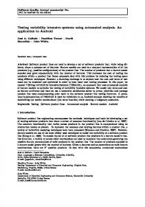
6.2 Cost of Generated Tests One of our objectives is to assess the reduction in cost brought by the DRPP algorithm. This raises two questions. Since we do not have cost data for test suites, what surrogate measure can we use? Second, assuming we have such a measure, what do we compare the results of DRPP with? Regarding the first question, we use test suite size, measured as number of executed methods, as a surrogate measure for cost. It is reasonable to expect the cost of developing and running test suites to be proportional to the number of methods executed. Though different methods usually entail varying costs, this is expected to average out over an entire test suite and is therefore considered a good approximation at the test suite level. As for the second question, we compare DRPP test suites with the algorithm by Karçali and Tai (KT) [23] which was briefly introduced in Section 2.1, as this is the only possible point of comparison in the literature. Test sequences were generated for all the different CSPE constraint criteria for a fixed CSPE constraint predicate criterion: Predicate Coverage. Since KT’s approach does not address the coverage of predicates and simply covers Possibly Valid constraints once, this point of comparison corresponds to our Predicate Coverage criterion. By fixing the CSPE constraint predicate criterion to Predicate Coverage, we thus make sure that we can compare the two techniques and investigate without bias whether the DRPP algorithm is good at minimizing test sequences. Using more complex predicate criteria would only increase the relative improvement of DRPP over KT. Sequences were therefore generated for A, AP-PC, NP-PC, and ANP-PC. Figure 6 is a chart depicting the size of the DRPP-based test sets and the size of the KT test sets on Petstore system in terms of number of methods executed in the test suites. The DRPP-based test sequences clearly show a significantly lower size for all criteria which corresponds to relative improvements ranging from 26% to 53% over the KT based test sequences. Recall that the Petstore case study does not include any Never Valid constraints; therefore the N test adequacy criterion is not applicable.

22


October 2005

250

Test Suite Cost

200

150

KarTai PrestoSequence

100

50

0 A

AP

NP

ANP

Criterion

Figure 6. Costs of DRPP-based vs. KT Test Sequences for Petstore The N criterion is of particular interest and in order to show this we repeat the test size analysis on another example component, the Queue component. The CSPE constraints based on this component do include Never Valid constraints. Figure 7 is a chart depicting the size of the DRPP and KT-based test sequences on the Queue case study. The relative improvements of DRPP over KT for criteria A, AP, NP, and ANP are consistent with the Petstore results (ranges from 26% to 54%). For the N criterion the DRPP-based approach shows no improvement as the sequences sizes are exactly the same (30 methods). The reason for this is that both approaches handle Never Valid constraints in the same way. Recall that the breadth first construction of a tree path, following KT algorithm, stops when a Never Valid constraint is encountered: this ends the tree path (i.e., test case) construction. When such a test case is executed and a Never Valid constraint, ending the test case, is reached, a new test case in the test suite has to be selected, requiring a reinitialization of the component. This is exactly what our algorithm is doing: the only way to leave an error node, e.g., after exercising a Never Valid constraint, is to re-initialize the component. 250

Test Suite Cost

200

150

KarTai PrestoSequence

100

50

0 A

AP

N

NP

ANP

Criterion

Figure 7. Costs of DRPP-based vs. KT Test Sequences for Queue

23


October 2005

6.3 Effectiveness of CSPE-based Tests Let us now turn to the analysis of the fault-detection effectiveness of our CSPE-based coverage criteria. Due to size constraints, the results reported here are for the most complete criterion: ANP-PC. From a practical standpoint we want to determine whether deriving such test suites based on interface method contracts brings any significant advantage over simpler test strategies. In order to investigate this question, a number of issues have to be addressed. Since we have no known faults on the component we use, how do we seed faults to allow ourselves to experiment? Second, with what other test strategy should we compare our CSPE results? It is common in testing research to resort to seeding faults to investigate the effectiveness of testing techniques [28]. The main reason is practical: researchers rarely have access to large numbers of actual faults. The question is now how to seed such faults in a systematic and unbiased manner? To do so, most researchers have used mutation operators [25] and recent results have shown this practice to be reasonably accurate [3]. However, in order to be as realistic as possible, we assumed that the component was correct to start with and that the application properly used the component interface. This is not necessarily the case in practice but should be representative in most situations with professional vendors and skilled users. Furthermore, as discussed above, in a component-based context, test cases (in our case CSPEbased test cases) are derived to investigate whether the component can work correctly on the selected platform, i.e., to investigate the impact of defects or discrepancies in the component platform (or other components) on the component under investigation. To do so, the most straightforward solution is to seed mutants in the component platform (or other components). This turns out to be at best very difficult because of the complexity of the deployment platform. Another simpler solution is to simulate platform failures (e.g., the platform fails to throw an exception), which is the approach we adopt here by simulating such failures directly in the component. A set of mutation operators were then selected and faults were seeded manually and randomly through the entire component code. The mutation operators were selected so as to potentially simulate component deployment failures. So, for example, interface mutation operators [21] were not selected as we assumed that the component application used correctly the component

24


October 2005

interface and that this interface was correct. In our experiment, we used both generic mutation operators [25] and others specifically defined for Java [24]. Table 2 lists the mutation operators that were used and the number of times each was seeded. Table 2. Types of Mutant Operator Types Used and the Number of Times Each was Seeded Operator Type

Count

AOR – Arithmetic Operator Replacement ROR – Relational Operator Replacement UOI – Unary Operator Insertion SDL – Statement Deletion CRP – Constant Replacement SVR – Scalar Variable Replacement EHR – Error Handler Removal Total

2 7 4 30 31 18 10 102

Furthermore, given our testing objective above and since the deployment platform involves the component container and a database, we selected mutants that could possibly lead to such deployment platform failures. Note that these mutants were manually seeded before any test suite was generated. For example, in the following mutant, a relation operator == is replaced with another relation operator >=: Original: if (orderState == OrderState.UNVERIFIED) Mutant: if (orderState >= OrderState.UNVERIFIED) The all methods and exceptions (AME) test strategy was used as a baseline of comparison to assess the effectiveness of the generated CSPE test suite. AME requires that all of the methods and all of the exception instances be covered at least once by a compliant test suite. An exception instance is defined as an exception type thrown by a method, i.e., the same exception type may be thrown by a number of methods and each one is an exception instance. AME [21] is a simple but thorough testing technique applicable without source code, and is therefore a good baseline of comparison. Out of the entire set of 102 mutants, 21 were identified as equivalent, 81 were killed by the CSPE test suite, and 76 were killed by the AME test suite. Therefore, the CSPE test suite killed all non-equivalent mutants, five more than the AME test suite. However, the number of methods executed in the 45 test cases of the CSPE test suite is 149, a much higher number than the 22 methods contained in the 5 AME test cases. The questions that now arise are: (1) How can we

25


October 2005

characterize the mutants killed only by CSPE and are they expected to correspond to critical, frequent faults in practice (Section 6.3.1)? (2) Can we decrease the cost of CSPE test suites while retaining (most of) their fault detection effectiveness (Section 6.3.2)? 6.3.1

Mutant Analysis

Regarding question (1), a careful analysis indicates that these mutants were all found in two specific areas of the Petstore component: where the order processing functionality (1 mutant) and the Petstore clear and confirm/cancel functionality (4 mutants) of the component are implemented. Both of these areas in the component share a common characteristic in that they implement part of the state-based behavior of the component. As an example, the clear and confirm/cancel functionality is used to clear the Petstore database of all the orders. This is done in two steps through the clearPetstore, and either the confirmClearPetstore or cancelClearPetstore methods. The clearPestore method returns a confirmation code, and

clearing the database requires that the same confirmation code be provided in the confirmClearPetstore method. In the same way, the clearing of the database can be revoked

by calling the cancelClearPetstore method with the confirmation code. (A set of confirmation codes is maintained in the component—attribute confirmCodes—and stored in the database.) This behavior can be modeled by the (incomplete) state diagrams in Figure 8 (transitions have been numbered for convenience). If a code does not exist when calling confirmClearPetstore or cancelClearPetstore (while the Petstore is not empty), then an exception is thrown (transition 2 or 3). [ confirmCodes ->exists (code )] confirmClearPetstore (code ) / confirmCodes .remove(code )

5

1

code=clearPetstore () / confirmCodes .add (code ) NON-EMPTY

2 [not confirmCodes ->exists(code)] cancelClearPetstore (code) / throwException ()

EMPTY

[confirmCodes ->exists(code)] cancelClearPetstore (code) / confirmCodes . remove(code)

4

3 [not confirmCodes ->exists(code)] confirmClearPetstore (code) / throwException ()

Figure 8. Statechart of the Petstore clearing functionality As a result of the mutants the incorrect behavior results in confirmClearPetstore and cancelClearPetstore failing to properly remove the valid confirmation code from the set of

26


October 2005

maintained codes after their execution. This corresponds in Figure 8 to removing the actions circled with dashed lines. As a result, if a call to confirmClearPetstore is made with a code that has already been used, for instance in a previous call to confirmClearPetstore, then transition 5 is taken clearing the database again. The second call to confirmClearPetstore should have triggered transition 3, resulting in an exception being thrown (the code exists in the set of valid codes when it should not). The Petstore can be cleared or the clearing can be cancelled multiple times with the same confirmation code. Note that these mutants emulate a deployment failure as this would correspond to a scenario where the container does not forward the request properly to the database or where the database would not properly remove the code from its records. The reason why only CSPE killed these mutants is that it ensures that the faulty behaviors were exercised (i.e., trying to execute confirmClearPetstore twice) whereas the AME technique only verifies the basic Petstore clearing functionality by asserting that the database is empty after a confirmClearPetstore with valid confirmation code, that it has been unaltered after a cancelClearPetstore with valid confirmation code, or that it has been unaltered and an

exception has been thrown after a confirmClearPetstore (or cancelClearPetstore) with an invalid confirmation code. If we now generalize, the mutants missed by AME and killed by CSPE are faults related to the state behavior of parts of the component and AME does not fully exercise this state behavior. From what we know on testing OO systems [7], detecting state behavior-related faults is crucial as many critical functionalities in such systems exhibit such behavior. Many test techniques relying on detailed design information or code are state-based [7] and are defined in terms of state model coverage. This clearly reflects the fact that detecting such faults is of practical importance. We can therefore conclude that our CSPE-based approach is likely to be useful in detecting certain types of faults, namely state-based faults, and this is going to be of practical importance. Note that our approach achieves such results without providing any explicit state model of the component to the user, as discussed in Section 2.3.

27


6.3.2

October 2005

Reducing the cost of CSPE-based test sets

If we now come back to question (2) above, can we find a way to select of subset of CSPE test cases that would retain a high fault detection effectiveness with a cost comparable to that of AME? To achieve this, we devised the following test case selection heuristic based on mutant analysis: 1. Seed representative mutants in the component (following the procedure described above); 2. Evaluate each individual CSPE test case with respect to its mutation score; 3. Order the test cases in descending score order; 4. Select the first n test cases, n being determined by available test resources. The idea is to use mutant analysis as an indicator of test cases with high fault detection capability so as to select them for testing. The tasks of creating and executing test suites on mutants can easily be automated, as done in this case study, and the effort overhead should therefore not be an issue. But the question remains of whether such a heuristic is likely to work in practice. Continuing with our case study, we determined based on the average number of methods per test case in CSPE and AME test suites, that we would need to select a subset of 7 CSPE test cases to ensure the size of the resulting test suite would not be larger than that of the AME test suite. In order to obtain realistic results, we needed to set up the experiment so that the heuristic would be based on a subset of mutants (learning set) and be evaluated on a different set (evaluation set). We randomly generated 10 pairs of such sets to be able to statistically compare the results of AME with those of CSPE subsets. Over 10 evaluation sets the average number of mutants killed by AME and CSPE were 37.9 and 40.5, respectively. Given that 40.5 is the maximum possible average6, 100% of the mutants were systematically killed by our subsets of 7 CSPE test cases whereas AME killed an average of 94% of the mutants. A statistical test of significance, whether using a paired t-test or a non-parametric Wilcoxon signed rank test [15], indicates that the difference is significant with a p-value < 0.0001. Furthermore, in terms of cost, the average number of methods in CSPE subsets was smaller than in the AME test suite: 19.2 and 22,

6

Five of the evaluation sets contain 40 mutants and another five contain 41 mutants. 28


October 2005

respectively. We can therefore conclude that the heuristic presented above can be effective at selecting a subset of CSPE test cases so as to significantly reduce its cost while retaining its fault detection capability.

7 CONCLUSION This report presented a systematic methodology for the testing of deployed COTS components based on a careful analysis of interface method contracts to generate interface method sequential constraints. This methodology does not require the component design or code but implies that the component vendor provides a specific test interface as part of the component’s public interface so as to allow the component to be controllable and observable, two basic testability requirements. This report also proposed an optimization algorithm to generate test sequences of minimal length to fulfill the proposed coverage criteria, thus reducing the cost of testing. A case study using mutation analysis, performed on a representative component, shows that the proposed test strategy is effective at killing mutants and that its cost can be significantly reduced by using a simple test selection heuristic based on mutation analysis. More precisely, a careful analysis revealed that it is particularly effective at killing mutants affecting the state behavior of parts of the component thus suggesting it is particularly effective at detecting state-related faults, a category of faults very common in object-oriented software.

ACKNOWLEDGEMENTS This work was partly supported by a Canada Research Chair (CRC) grant. Lionel Briand and Yvan Labiche were further supported by NSERC operational grants. This work is based on M. Sówka’s Masters thesis and is part of a larger project (www.sce.carleton.ca/Squall).

REFERENCES [1] [2]

R. K. Ahuja, T. L. Magnanti and J. B. Orlin, Network flows : theory, algorithms, and applications, Prentice Hall, 1993. P. Ammann, J. Offutt and H. Huang, “Coverage criteria for logical expressions,” Proc. IEEE International Symposium on Software Reliability Engineering, pp. 99-107, 2003.

29


[3]

[4] [5]

[6] [7] [8] [9] [10]

[11]

[12] [13] [14]

[15] [16] [17] [18] [19] [20] [21]

[22]

October 2005

J. H. Andrews, L. C. Briand and Y. Labiche, “Is Mutation an Appropriate Tool for Testing Experiments?” Proc. IEEE International Conference on Software Engineering, pp. 402411, 2005. M. O. Ball and M. J. Magazine, “Sequencing of Insertions in Printed Circuit Board Assembly,” Operations Research, vol. 36 (2), pp. 192-201, 1987. S. Beydeda and V. Gruhn, “An integrated testing technique for component-based software,” Proc. IEEE International Conference on Computer Systems and Applications, pp. 328-334, 2001. S. Beydeda and V. Gruhn, Testing COTS Components and Systems, Springer, 2005. R. V. Binder, Testing Object-Oriented Systems, Addison-Wesley, 1999. R. G. Busacker and P. J. Gowen, “A Procedure for Determining a Family of Minimal-Cost Network Flow Patterns,” John Hopkins University, O.R.O. Tech. Paper 15, 1961. P. M. Camerini, L. Fratta and F. Maffioli, “Ranking arborescences in O(Km log n) time,” European Journal of Operational Research, vol. 4 (4), pp. 235-242, 1980. R. H. Carver and K.-C. Tai, “Use of sequencing constraints for specification-based testing of concurrent programs,” IEEE Transactions on Software Engineering, vol. 24 (6), pp. 471-490, 1998. A. Cechich and M. Polo, “Use of Sequencing Constraints for Specification Based Testing of Concurrent Programs,” in S. Beydeda and V. Gruhn, Eds., Testing COTS Components and Systems, Springer, pp. 71-88, 2005. N. Christofides, V. Campos, A. Corberan and E. Mota, “An algorithm for the rural postman problem on a directed graph,” Mathematical Programming Studies (26), pp. 155-66, 1986. A. Corbéran, G. Mejía and J. M. Sanchis, “New Results on the Mixed General Routing Problem,” Operations Research, vol. 53 (2), pp. 363-376, 2005. F. J. Daniels and K. C. Tai, “Measuring the effectiveness of method test sequences derived from sequencing constraints,” Proc. Technology of Object-Oriented Languages and Systems, pp. 74-83, 1999. J. L. Devore, Probability and Statistics for Eng. and the Sciences, Duxbury Press, 5 Edition, 1999. M. Dror, Arc Routing: Theory, Solutions and Applications, Kluwer, 2000. J. Edmonds, “Optimum branchings,” J. Res. Nat. Bur. Standards Sect. B, vol. 71B, pp. 233-240, 1967. Fleury, “Deux problemes de geometrie de situation,” Journal de mathematiques elementaires, pp. 257-261, 1883. U. S. FTF, UML 2.0 Superstructure Final Adopted Specification, http://www.omg.org/cgibin/doc?ptc/2003-08-02, (Last accessed 26 Jan. 2005) J. Z. Gao, H.-S. Jacob Tsao, Ye Wu, Testing and Quality Assurance for Component-based Software, Artech House, 2003. S. Ghosh and A. Mathur, “Interface Mutation to assess the adequacy of tests for components and systems,” Proc. International Conference on Technology of ObjectOriented Languages and Systems, pp. 37-46, 2000. JBoss, JBoss Application Server, http://www.jboss.com, (Last accessed 26 Jan. 2005)

30


October 2005

[23] B. Karçali and K.-C. Tai, “Automated test sequence generation using sequencing constraints for concurrent programs,” Proc. International Symposium on Software Engineering for Parallel and Distributed Systems, pp. 97-108, 1999. [24] S. Kim, J. A. Clark and J. A. McDermid, “Class Mutation: Mutation Testing for ObjectOriented Programs,” Proc. Net.ObjectDays, 2000. [25] K. N. King and A. J. Offutt, “A Fortran language system for mutation-based software testing ” Software. Practice and Experience. , vol. 21 (7 ), pp. 685-718 1991 [26] J. K. Lenstra and A. H. G. Rinnooy-Kan, “Complexity of vehicle routing and scheduling problems,” Networks, vol. 11, pp. 221-227, 1981. [27] V. Massol and T. Husted, JUnit in Action, Manning Publications Co., 2004. [28] A. J. Offutt, “A practical system for mutation testing: help for the common programmer,” Proc. Proceedings of International Test Conference, pp. 824-30, 1994. [29] J. B. Orlin, “A polynomial time primal network simplex algorithm for minimum cost flows,” Proc. ACM-SIAM Symposium on Discrete Algorithms, pp. 474-481, 1996. [30] A. Orso, M. J. Harrold, D. Rosenblum, G. Rothermel, M. L. Soffa and H. Do, “Using component metacontent to support the regression testing of component-based software,” Proc. IEEE International Conference on Software Maintenance, pp. 716-725, 2001. [31] T. J. Ostrand and M. J. Balcer, “The Category-Partition Method for Specifying and Generating Functional Test,” Communications of the ACM, vol. 31 (6), pp. 676-686, 1988. [32] A. Polini and A. Bertolino, “A User-Oriented Framework for Component Deployment Testing,” in S. Beydeda and V. Gruhn, Eds., Testing COTS Components and Systems, Springer, 2005. [33] D. S. Rosenblum, “Adequate testing of component-based software,” Department of Information and Computer Science, University of California Technical Report 97-34, 1997. [34] Sun Microsystems, Enterprise JavaBeans Technology, http://java.sun.com/products/ejb/, (Last accessed 26 Jan. 2005) [35] Sun Microsystems, Java Blueprints, http://java.sun.com/reference/blueprints/, (Last accessed 26 Jan. 2005) [36] C. Szyperski, with Dominik Gruntz and Stephen Murer, Compnent Software – Beyond Object-Oriented Programming, Component Software, Addison-Wesley, 2nd ed., 1999. [37] R. E. Tarjan, “Finding optimum branchings,” Networks, vol. 7 (1), pp. 25-35, 1977. [38] J. Warmer and A. Kleppe, The Object Constraint Language, Addison Wesley, 2nd ed., 2003. [39] E. Weyuker, “Automatically Generating Test Data from a Boolean Specification,” IEEE Transactions on Software Engineering, vol. 20 (5), pp. 353-363, 1994. [40] L. C. Briand, Y. Labiche and H. Sun, “Investigating the Use of Analysis Contracts to Improve the Testability of Object-Oriented Code,” Software - Practice and Experience, vol. 33 (7), pp. 637-672, 2003.

31


Appendix A

October 2005

The Queue Example (complete data)

Table 3 shows the complete list of (56) CSPE constraints for the Queue example discussed in Section 4.4, using labels instead of complete predicates. The exact CSPE constraint predicates p1 to p6 can be found in Table 4. Table 3. CSPE constraints for the Queue c1=(#,init,true) c2=(#,empty,false) c3=(#,eque,false) c4=(#,dque,false) c5=(#,top,false) c6=(#,getLock,p2) c7=(#,rlsLock,p3) c8=(init,init,false) c9=(init,empty,true) c10=(init,eque,p1) c11=(init,dque,false) c12=(init,top,false) c13=(init,getLock,p2) c14=(init,rlsLock,p3) c15=(empty,init,false) c16=(empty,empty,true) c17=(empty,eque,p1) c18=(empty,dque,p4) c19=(empty,top,p5)

c20=(empty,getLock,p2) c21=(empty,rlsLock,p3) c22=(eque,init,false) c23=(eque,empty,true) c24=(eque,eque,p1) c25=(eque,dque,p1) c26=(eque,top,true) c27=(eque,getLock,p2) c28=(eque,rlsLock,p3) c29=(dque,init,false) c30=(dque,empty,true) c31=(dque,eque,p1) c32=(dque,dque,p4) c33=(dque,top,p5) c34=(dque,getLock,p2) c35=(dque,rlsLock,p3) c36=(top,init,false) c37=(top,empty,true) c38=(top,eque,p1)

c39=(top,dque,p1) c40=(top,top,true) c41=(top,getLock,p2) c42=(top,rlsLock,p3) c43=(getLock,init,false) c44=(getLock,empty,true) c45=(getLock,eque,p1) c46=(getLock,dque,p4) c47=(getLock,top,p5) c48=(getLock,getLock,false) c49=(getLock,rlsLock,p6) c50=(rlsLock,init,false) c51=(rlsLock,empty,true) c52=(rlsLock,eque,p2) c53=(rlsLock,dque,p3) c54=(rlsLock,top,p5) c55=(rlsLock,getLock,p2) c56=(rlsLock,rlsLock,false)

Table 4. CSPE constraint predicates for the Queue Predicate Literal p1 p2 p3 p4 p5 p6

Constraint Predicate lock->isEmpty() or (lock = l) lock->isEmpty() lock->isEmpty() and (lock = l) (size 0) and ( lock->isEmpty() or (lock = l) ) size 0 lock = l

32


Appendix B

October 2005

Algorithm Details

The Directed Rural Postman Problem is an extension of the Chinese Postman Problem, which in turn is similar to the well-known Traveling Salesman Problem7. The book edited by Mosh Dror [16] provides a comprehensive review of such graph routing problems and solutions, and the reader is referred to it for further details on the above-mentioned problems. In the formulation of the Directed Rural Postman Problem (DRPP) the directed graph denoted by

G = ( N , A) contains a set of nodes N, and a set of arcs A of costs cij ≥ 0 . (Note that this constraint on costs is satisfied in our application problem.) The set of arcs A contains a subset of arcs AR ⊆ A that are referred to as required arcs. In the DRPP only the required arcs need to be traversed at least once, and all the other arcs do not necessarily have to be traversed, but may be traversed if they are needed to create the shortest possible path in the solution to the problem. Figure 9 is a small example of a graph demonstrating the DRPP. The graph contains four arcs, a1 through a4, and three nodes, n1 through n3. Arcs a1 and a3 are the only two required arcs, displayed as solid lines. An example path solution to the DRPP on this graph is [a1, a4, a2, a3]. Note that although the arcs a2 and a4 are not required they are used in the solution in order to be able to traverse all the arcs that are required (arcs a1 and a3). a1 :1

n1

a2 :2

n2

a3 :2

n3

a4 :1

Figure 9. Directed Rural Postman Problem Example Graph

The DRPP is NP-Complete [26], and as such does not have a polynomial time solution and is generally not easy to solve. The solution to the DRPP used in this report is adapted from [12],

7

The Traveling Salesman Problem is to find the shortest way of visiting all the cities from a graph showing cities as nodes and indicating the travel costs between cities on nodes. In the Chinese Postman Problem, on the other hand, it is required that all the arcs of the graph be traversed at the lowest cost possible. 33


October 2005

which is first detailed in Section B.1. Our adaptation of Christofides’ solution is then detailed in Sections B.2, B.3 and B.4.

B.1 Christofides’ Solutions to the DRPP problem A heuristic solution and an exact algorithm for solving the DRPP are presented in [12]8, simply referred to as Christofides’ solution. Using the exact algorithm, Christofides et al. were able to solve DRPP for |N| ranging from 13 to 80, and |A| ranging from 24 to 180. We decided to adapt the heuristic solution, which is based on graph theory, instead of the exact solution, in order to have a more general (scalable), although not always optimal, solution, especially since, according to experimental evidence reported by Christofides, the heuristic graph-based solution is reasonably close to the optimal. (The reader is referred to [12] for further details on this experimental evidence and on the integer linear programming problem specification.) We will however consider in future work the exact solution to the DRPP by Christofides [12], as well as other more recent solutions9 to the DRPP [13]. The objective of the DRPP solution by Christofides is to identify which of the non-required arcs will be used in the final solution to the DRPP, and how many times each of the arcs of the entire set of arcs will be traversed. The graph based solution consists eventually in finding an Euler tour in an Eulerian graph. In order to do so, the initial graph (which is our case represents CSPE constraints) has to undergo a set of four initial transformations (Section B.2) and then be made Eulerian (Section B.3). Section B.4 then shows how an Euler tour can be determined and why the Euler tour is a solution to the DRPP problem. Broadly speaking, the graph transformations below aim at promoting non-required arcs to the set of required arcs because, based on observation provided in [12], they will be part of any solution to the DRPP. Then the graph containing only those required arcs (either part of the original set of required arcs or promoted) is ensured to be Eulerian and an Euler tour is found. 8

This DRPP solution was applied to printed circuit board manufacturing [4]. The article by Corbéran et al. presents an advanced solution to the mixed general routing problem, where the DRPP is a special case of such a problem. 9

34


October 2005

B.2 Initial Transformations First, recall that the required arcs, denoted as AR, are identified by the targeted functionalities and the selected CSPE predicate coverage criterion. Any node in the graph that is not the source or the target of at least one required arc is not a required node. There is one exception to this rule, namely the node labeled #. This node corresponds to the initialization of the component and will start any test case used to test the component, i.e., it must be part of the solution. Node labeled # is thus always a required node. Additionally, since the only arcs leaving error nodes are those labeled ‘~’, those arcs are required arcs. We thus identify in G=(N,A) a set of required nodes AR and a set of required nodes NR. Second, it is worth mentioning that because of our definition of the initial graph, i.e., the way we build nodes and arcs, and especially the re-initialization arcs, the initial graph is strongly connected. Additionally, if only considering the required arcs, the initial graph may be component disconnected. The purpose of the initial transformations is to find paths in the original graph, made of required and non-required arcs, that will facilitate (because they are the shortest path between two nodes) the identification of a nearly optimal solution. In order to ease reading in this section, the graph transformation steps numbers are indicated as superscripts to G (the graph), N (the set of nodes) and A (the set of arcs): e.g., graph G1=(N1,A1) is the result of the first transformation on graph G=(N,A). Transformation Step 1—Prune Non-required Nodes and Arcs: Remove all nodes that do not have at least one adjacent a ∈ AR and all arcs that are not in AR . The resulting graph is denoted as G1 = ( N R1 , AR1 ) . ( N1R ⊆ N and A1R = A R .) The next step of the transformation adds additional arcs, which are referred to as virtual arcs, to the directed graph G1 . Virtual arcs are used to record the cheapest path in G (the original graph) between every ordered pair of nodes in G1 (i.e., required nodes), and can represent either a single arc or a path formed by a sequence of arcs of graph G. These paths can potentially help finding a cheap solution to the DRPP problem: it may be cheaper to traverse non-required nodes and arcs (i.e., a path in G) rather than traversing only required nodes and arcs (i.e., in G1 ).

35


October 2005

Transformation Step 2—Add Virtual Arcs10: Construct a graph G 2 by adding virtual arcs between every ordered pair of nodes (i, j ) ∈ N R1 . The cost of virtual arc c(i , j ) is equal to the lowest cost path V(i,j) in G between required nodes i

(

)

and j. The resulting graph is denoted as G 2 = N R2 , A 2 , where N R2 = N R1 , A 2 = A1R ∪ AV2 , and 2 V

A is the set of new virtual arcs. The graphs of Figure 10 illustrate the first two steps of the graph transformation. Required arcs are drawn with solid lines, non-required arcs are draw with dashed lines, and virtual arcs are drawn with dotted lines. Figure 10 (a) shows the original graph G. In step 1, non-required arcs (a3, a4, a5, a6) and non-required node (n4) are removed from G. The result is graph G1 shown in Figure 10 (b). Virtual arcs are then added to graph G1, based on the shortest paths in the original graph G, and the resulting graph G2 is shown in Figure 10 (c). For example: Virtual arc a9 (cost 1) corresponds to path [a1] of cost 1 in G (there are other paths in G from n1 to n2 but of higher costs); Virtual arc a8 (cost 2) corresponds to path [a5, a6] (both cost 1); Virtual arc a12 (cost 3) corresponds to path [a5, a6, a1] in G (all cost 1).

a 7:1

a 8:2

a 2:3

a 2:3

a1 :1

a1 :1

n2

a 12:3 a 11 :3

a 2:3

:1 a4

a 3:1

a 10:2

1

n4

a 9:1

n2

a6:

n2

n1 a1 :1

n1

n1

:1 a5

n3

n3

n3

(a) Original Graph G (b) Graph G1 after Step 1 (c) Graph G 2 after Step 2 Figure 10. The First Two Steps of Graph Transformation

In the third transformation, redundant virtual arcs are identified. A virtual arc is redundant when we can find a path in G2 between the same two nodes (including required and/or non required arcs) of the same cost.

10

Note that the mapping between virtual arcs and the corresponding path of non-required (and/or required) arcs in the original graph is recorded. Eventually, if a virtual arc is used in the solution to the DRPP, it will be expanded and replaced by the corresponding path in the original graph to form a complete, concrete test case. 36


October 2005

Transformation Step 3—Remove Redundant Virtual Arcs: From the set of virtual arcs AV2 of graph G 2 remove: (a) any arc (i, j ) ∈ AV2 for which there exists k ∈ N R2 such that cij = cik + ckj; (b) any arc (i, j ) ∈ AV2 such that there exists a required arc in AR2 from node i to node j. (Note that transformations (a) and (b) are repeated until no further removal is possible.)

(

)

The resulting graph is denoted as G 3 = N R3 , A3 , where N R3 = N R1 , A3 = A1R ∪ AV3 , and AV3 is the reduced set of virtual arcs. The two graphs of Figure 11 illustrate transformation 3 from graph G 2 in Figure 10 (c). In Figure 11 (a), an arc that meets condition (a) is identified (an ‘X’ crosses the arc): arc a12 is redundant with the sequence of arcs a8 and a1. In Figure 11 (b), arcs that meet condition (b) are identified: arc a11 is redundant with required arc a2, and arc a9 is redundant with required arc a1.

a 8:2

a 2:3

n3

a 11 :3

a12:3

a 11 :3

a 2:3

a 7:1

n2

a 7:1

a 8:2

a 10:2

n2

a 9:1

a 10:2

a1 :1

n1 a 9:1

a1 :1

n1

n3

(a) Transitive-equivalent Arcs Removed (a) Arcs Equivalent to Required Arcs Removed Figure 11. Third Step of the Graph Transformation

After redundant virtual arcs have been removed, between each pair of required nodes there is either (a) a required arc, or (b) a virtual arc representing the shortest path in G made of required and non-required arcs between the two nodes, or (c) both a required arc and a virtual arc in which case we have found a cheapest way than the required arc to go from its source to target node.

(

)

The resulting graph G 3 = N R3 , A3 is strongly connected. The graph induced by the required set

(

)

of arcs only, i.e., N R3 , A1R , may be component disconnected. We refer to this graph as being component disconnected with respect to (w.r.t.) required arcs and we denote it as Gcd3 . In the rest

37


October 2005

of the text, unless otherwise specified, a graph that is component disconnected w.r.t. the required arcs is simply called component disconnected. The component disconnected graph Gcd3 is partitioned into components C1,…,Cp and can be

(

)

3 represented in a condensed way by graph GC3 = N C3 , AVC , such that the nodes of such graph

represents the component Ci in graph Gcd3 , and the only arcs between those nodes correspond to some of the virtual arcs of the not condensed graph. The example graph of Figure 12 (a) is a component disconnected graph ( Gcd3 ) made of two components C1 and C2. Component C1 is strongly connected, while component C2 is not. The corresponding condensed graph is shown in Figure 12 (b) where only the virtual arcs spanning the two components C1 and C2 are involved. C1

a1

c1 a3

a4

C2

a3

a4

a2

a1

c2 3 (b) Condensed Graph GC3 (a) Component Disconnected (w.r.t. required arcs) Graph Gcd Figure 12. Component Disconnected Graph and Corresponding Condensed Graph, an

Example

The last step of the graph transformation promotes virtual arcs from set AV3 to required arcs set AR3 , because they will be involved in any solution to the DRPP, and is based on two observations

presented in [12]. First, if for two components Ci and Cj in the component disconnected graph the unique arc from Ci to Cj is a virtual arc, then this virtual arc must be in any solution to the DRPP. Second, if the only way to reach or leave a required node in a component is to take a virtual arc, then again, this virtual arc must be in any solution to the DRPP. The reason for these arc promotions is that only required arcs are traversed in the final solution, if there is only one arc connecting a component or node then it must be a required arc. 38


October 2005

Transformation Step 4—Promote Virtual Arcs: Virtual arc (i, j) is promoted from AV3 to the set of required arcs if it meets any one of the following three conditions: there is a partition of G3 into two components Ci and Cj such that (i,j) is the unique (a) arc of Ci to Cj; (b) (i,j) is the only arc directed out of node i ∈ N R3 ;

(c)

(i,j) is the only arc directed into node j ∈ N R3 .

(

)

The resulting graph is G 4 = N R4 , A 4 , where N R4 = N R1 , A 4 = A1R ∪ AR4new ∪ AV4 , and AR4new is the set of promoted virtual arcs ( AR4new ∪ AV4 = AV3 ). AV4 is the reduced set of virtual arcs. The set of required arcs in G4 is AR4 = A1R ∪ AR4new . For example, in the graph of Figure 12 (a), two virtual arcs a1 and a2 are promoted into the set of required arcs according to transformation step 4. Arc a1 is the only arc that is directed out of component C1 and into component C2 whereas arc a2 is the only arc directed into its target node. The promotion of virtual arcs into required arcs in the last step does not guarantee that G4 is not component disconnected w.r.t. to required arcs. We however have to ensure it is strongly connected w.r.t. required arcs and symmetric, i.e., it is Eulerian. Making the graph strongly connected and symmetric is the objective of the following section.

B.3 Connected and Symmetric (i.e., Eulerian) Graph These additional transformations of the graph, to make it Eulerian, are mentioned in [12] but without any details as to how to proceed. Graph theory can help us find problems, and thus algorithms, to transform G4 into a connected (Section B.3.1) and symmetric (Section B.3.2) graph with respect to required arcs. B.3.1 Towards a Connected Graph: The Shortest Spanning Arborescence Problem

The shortest spanning arborescence problem (SSA) [17] is based on a directed graph G = ( N , A) . The problem is stated as follows: starting from a root node tα ∈ N , a set of arcs Asol ⊂ A must be chosen such that there exists paths from the root node to every other node of

39


October 2005

the graph with the lowest possible cost of the whole arborescence11. (Note that this does not necessarily mean that the paths from the root node of the arborescence to the leaf nodes are the shortest.) The selection of the root node tα from the set of nodes N depends on the context in which the SSA problem is applied to. An example of a shortest spanning arborescence is depicted in Figure 13, where the set of arcs Asol is highlighted. The solution to the SSA is the set of arcs Asol = {a1, a2, a4, a6, a7} with a total cost of 5. A set of arcs {a1, a3, a5, a8, a9} also connects the arborescence rooted at tα, but is not a SSA since its total cost is 13. ta a1:1

a2:1 a3:3

a4:1

a5:3

a6:1

a8:3

a7:1 a9:3

Figure 13. Example of Shortest Spanning Arborescence

Acknowledging that graph G4, obtained after the four initial transformations is potentially component disconnected (w.r.t. required arcs), our use of the SSA is to find a cost-effective way of making it connected. We will see that this is required for the next step of the transformations, i.e., to make the graph symmetric. In the case G4 is already connected then the current step is not required. Otherwise, as already mentioned, G4 can be represented by a condensed graph GC4 . We solve the SSA on GC4 , with root node tα as the component that contains node labeled #. This is a heuristic, based on a theory that node labeled # is the most connected node, and as already mentioned, node labeled # will start any of the test cases produced. The arcs of the SSA solution, Asol, are then promoted from the set of virtual arcs to the set of required arcs. The SSA is used to

tell us which arborescence is the cheapest, i.e., which virtual arcs in GC4 will likely be part of the oprimal solution, and thus should be promoted as required arcs.

11

The solution to the SSA was first presented by Edmunds in [17], and a better alternative solution, based on the work of Tarjan [37], can be found in [9]. 40


October 2005

Transformation Step 5—Promote Virtual Arcs from the SSA solution:

Determine the Shortest Spanning Arborescence on the condensed graph GC4 , generated from G4, and promote the virtual arcs that are part of the solution to the SSA problem.

(

)

The resulting graph is G 5 = N R5 , A5 , where N R5 = N R4 , A5 = AR4 ∪ AR5new ∪ AV5 , and AR5new is the set of promoted virtual arcs because part of the SSA solution ( AR5new ∪ AV5 = AV4 ). AV5 is the reduced set of virtual arcs. The set of required arcs in G5 is AR5 = AR4 ∪ AR5new . The graph of Figure 14 (a) is an example of graph G4 which is component disconnected. Figure 14 (a) shows what the components are. The virtual arcs labeled a through d (identifying them in this example, as otherwise they are not labeled) are the arcs used to find the Shortest Spanning Arborescence. In this simple example the shortest spanning arborescence rooted at the node containing # is formed by the arcs a and b. These arcs are then promoted to required arcs making the graph G5 connected (w.r.t. required arcs): Figure 14 (b). #

#

d:5

a:3

d:5

a:3

c:5

c:5 b:3

(a) Component Disconnected Graph G

b:3

4

(b) Connected Graph G5 Figure 14. Connecting (w.r.t. required arcs) using SSA (re-initializing arcs are omitted) B.3.2 Towards a Symmetric Graph: The Minimum Cost Maximum Flow Problem

Recall that our overall objective is to build a graph made of required arcs and required nodes that is Eulerian (connected and symmetric). The subgraph of G5 containing only required arcs and nodes is connected (this is ensured by the previous transformation) but not necessarily symmetric. If it is symmetric, then the transformation described in the current section is not necessary. In this section we first introduce the Minimum Cost Maximum Flow (MCMF) problem (Section B.3.2.1). Then we show how we use a solution to the MCMF problem to make our graph

41


October 2005

symmetric with respect to required arcs (Section B.3.2.2), i.e., the in-degree and out-degree when only accounting for required arcs are equal for all the required nodes. B.3.2.1 Minimum Cost Maximum Flow

The minimum cost maximum flow (MCMF) problem is a variation of the maximum flow family of problems reviewed in [1]. The variation of the MCMF problem used in this report is known as the supply and demand problem. In this kind of problem, a directed graph is seen as a flow network and used to solve problems about flow of goods between locations (i.e., nodes) where those goods are produced (supply) and where they are used (demand). The solution accounts for quantities that are produced and used by the supply and demand nodes (through a solution to the maximum flow), but also for the cost it takes to send trucks on specific routes (by making the flow minimum cost). In other words, we have a directed graph G = ( N , A) , where the nodes are either of the source type, n ∈ N r , associated with a positive value (supply), or sink type, n ∈ N s , associated with a negative value (demand). In the supply and demand problem, it is required that arcs are assigned a flow value such that source nodes have a net flow directed out equal to their supply (producers of goods sell all their stock), and sink nodes have a net flow directed in equal to their demand (users receive what they need), at the lowest possible cost. The graph G = (N0, A0) specifying the flow problem contains supply and demand nodes. These nodes are labeled by the quantities produced and used. The arcs are labeled with how much a unit of flow costs. In order to solve the supply and demand problem this graph defining the flow is modified into graph G1 = (N1, A1). First, two additional arcs are added to the set of nodes: root source node r and root sink node s. Then, so called utility arcs (set Au) are added from r to all the supply nodes and from all the demand nodes to s. The utility arcs are labeled by capacities, indicating the maximum flow that can go through them: the capacity is thus set to the arc’s target node quantity (for an arc leaving the root source node) or the arc’s source node quantity (for an arc going to the root sink node). The utility arcs are not assigned any cost (rather the cost is 0) and the original arcs have an unlimited capacity.

42


October 2005

An r-s flow is then defined as a set of paths V(r,s) from r to s. A flow value f(i,j) is defined as the number of times arc (i,j) appears in the r to s flow, i.e., in the paths of the flow. The cost of the rs flow that is to be minimized is defined as the sum of the products of each of the arc’s flow

value and cost: costr -s =

∑

( i , j )∈ Ao

f ( i , j ) c( i , j ) . At the end of the solution of the supply and demand

problem, root source node r, root sink node s, and their adjacent arcs are removed, such that source nodes are left with a net flow directed out and sink nodes a net flow directed in. An example of the MCMF problem and solution is illustrated in Figure 15, which shows graph G1. Nodes with positive values (supply) are the source nodes {n1, n2, n3}, and nodes with

negative values (demand) are the sink nodes {n4, n5}. Arcs a1 through a7 are the arcs of Ao, and the arcs adjacent to nodes r and s are the arcs of Au. A solution to the MCMF problem of Figure 15 is an r-s flow where the path [r, n2, n5, s] appears twice, path [r, n1, n4, n5, s] appears three times, path [r, n3, n4, s] appears 4 times, and path [r, n3, n4, n5, s] once. The flow on the arcs of Ao is: {fa1=0, fa2=0, fa3=3, fa4=0, fa5=2, fa6=5, fa7=4}, and each of the node’s supply or demand is met. ::2

a1:3

n1:3

n2:2

::3

r

a2:1

a3:4

s

a5:1

a4:1

::6

::5 n3:5

a6:3

n4:-4

a7:3

n5:-6

::4

Figure 15. Directed Graph of a Minimum Cost Maximum Flow Problem

A solution to the MCMF problem was presented by Busackar and Gowen in [8]. This algorithm is advantagous because of its simplicity, but requires that all arc costs be non-negative (which is our case for building CSPE component test cases). Other fast solutions to the problem include those by Ahuja, Golderg, Orlin, and Tarjan [1]; and Orlin [29]. B.3.2.2 Use of MCMF to Make a Graph Symmetric

43


October 2005

In order to make a non-symmetric graph symmetric w.r.t. to the required arc set we need to duplicate some of the existing arcs and possibly promote some more of the virtual arcs to the required arc set such that every node as an equal in degree and out degree w.r.t. required arcs. The difficulty with this is that duplicating arcs in order to make one node of the graph symmetric has an effect on the net degree of the node on the other end of the arc. This indeed becomes a difficult problem. The MCMF is used to tell us which arcs have to be duplicated in order to make the graph symmetric and do this with a minimum cost of the arcs duplicated. Graph G5, result of the previous transformation (Section B.3.1), is used to solve a MCMF problem. Recall that the nodes of G5 are required nodes, and that its arcs are required arcs or virtual arcs. Costs associated with arcs in G5 are the cost associated with the corresponding CSPE constraints: either the cost of a required arc in G, i.e., the arc in G5 corresponds to one CSPE constraint, or the sum of the costs of the path in G represented by a virtual are or a promoted virtual arc in G5. Source and sink nodes, and their quantities (either supply or demand), are determined with respect to only required arcs. For each node n in G5 we compute D(n ) = d in (n ) − d out (n ) Where din(n) and dout(n) are the in degree and out degree of n when counting only required arcs. If D(n)0 then node n is

considered a source with supply equal to D(n). Otherwise, i.e., if D(n)=0, the node is already symmetric (with respect to required arcs): it is neither a sink or source. Figure 16 illustrates this. In Figure 16 (a), node m has two incoming required arcs (i.e., din(m)=2) and one outgoing required arcs (i.e., dout(m)=1), making it a supply node of quantity 1 (i.e., din(m)-dout(m)=2-1). Node n has one incoming required arc (i.e., din(n)=1) and three outgoing required arcs (i.e., dout(n)=3), making this node a demand node of quantity 2 (i.e., din(n)-dout(n)=1-3). Note that the presence of a virtual arc from node m to node n in Figure 16 (b) does not change the kind of those nodes and their quantities as only required arcs are accounted for. Figure 16 (a) and Figure 16 (b) are the two main situations that we can encounter and are worth discussing here: i.e., a source node is linked to a sink node. Other situations like the one in Figure 16 (c), where two symmetric nodes appear in the path from m to n, also (in the end) entail a source node and a sink node.

44


October 2005

When solving the MCMF problem, we connect sink nodes to the root sink node and the root supply node to supply nodes (Figure 16) and we account for the whole graph, i.e., we account for both required and virtual arcs, and consider that arcs have infinite capacities. This means that the maximum flow solution can involve required arcs as well as virtual arcs. r ::1

r s

:: 1

::2 m:1

s

::1

::1

::2

n:-2

m:1

:1

n:-2

:1

(a)

(b) r

:0

:0

s

:: 1

::2 m:1

n:-2

:1

(c) Figure 16. Preparing the graph for MCMF

Figure 17 illustrates the MCMF solution from Figure 16 (a). A first flow of capacity 1, labeled f1 starts from root node r, goes through nodes m and n and stops at root node s: Figure 17 (a). This results in the supply of node m being reduced by 1 (it is now 0) and the demand of node n augmented by 1 (it is now -1). Another flow, labeled f2 in Figure 17 (b) is necessary to meet the demand of n. This flow of capacity 1 starts from r, goes through the unlabeled node and then m and n, and stops at s. This results in the supply of the unlabeled node reduced by 1 and the demand of node n augmented by 1 (it is now 0). (Note that the supply of m has not changed because m is only traversed by the flow, instead of being its source.) In the end, the total flow through arc m-n is 2. r ::1

r

f1=1 f1=1 ::2

::1 m:0

f1=1

s f2=1 ::1

f1=1 ::1 m:0

n:-1 :0

:1

f2=1 f1=1

f2=1

(b)

(a) Figure 17. MCMF flows from Figure 16 (a)

45

f2=1 f1=1 ::2 n:0

s


October 2005

Figure 18 illustrates the MCMF solution from Figure 16 (b) in which we have added costs for the two arcs between m and n: the required arc costs 2 whereas the virtual arc costs 1. This time, because MCMF tries to minimize the cost of the maximum flow, the two flows f1 and f2 go through the virtual arc, instead of the required arc. This results in a flow for required arc m-n of 0 and a flow of 2 for virtual arc m-n. r ::1

f1=1

f1=1 :1

r

f1=1 ::2

::1 m: 1

:2

s

f2=1

::1

f1=1

f1=1 : 1 f2=1

m: 1

n:-2 :1

:1

f1=1 f2=1 ::2

::1 :2

s

n:-2

f2=1

(b)

(a) Figure 18. MCMF flows from Figure 16 (b)

In the solution to the MCMF problem, the flow on (required and virtual) arcs indicate where to add arcs, which arcs have to be added, and how many arcs have to be added. Consider for instance the flow result in Figure 17 (b). The flow on arc m-n is two, indicating that two new arcs (i.e., the arc flow) has to be created between m and n. Indeed, if two other arcs exist from m to n, then n has three incoming required arcs and three outgoing required arcs. Additionally, m then has three outgoing required arcs and three incoming required arcs, because one incoming required arc to m has a flow of one indicating that a new incoming arc to m is needed. In this case, the arcs to be added between m and n are necessarily duplicates of the required arcs because m and n are only linked by a required arc12. (We cannot create arcs that do not correspond to CSPE constraints.) Consider now the flow result in Figure 18 (b). The flow on required arc m-n is 0 which, according to what precedes, indicates that required arc m-n is not duplicated. The flow of two is instead on the virtual arc m-n, because the virtual arc has a lower cost than the required arc. In such a case, the virtual arc is promoted to a required arc and duplicated once (i.e., the virtual arc flow minus one). This again results in a total of three (required) arcs between m and n, making those nodes symmetric. Note the number of duplicates is the arc flow minus one because we already promote it once, i.e. the nodes to which it is adjacent have already been adjusted once.

12

Note that in the case of the example of Figure 16 (c), the flow of all the required arcs in the path from m to n will be two, leading to two duplications of these required arcs. All the nodes are then symmetric. 46


October 2005

As a result of the last transformation, summarized below, the graph made of the required nodes and required arcs is connected and symmetric, i.e., it is Eulerian. Transformation Step 6—Duplicate and Promote Arcs from the MCMF solution: Determine the MCMF solution from graph G5 according to the following settings: A sink node n is a node for which D(n ) = d in (n ) − d out (n ) 0, where din and dout only account for required arcs. Account for the whole graph, i.e., all its nodes and arcs in the MCMF solution. Arcs have infinite capacities. From the solution to the MCMF: A required arc with a flow of x is duplicated x times. A virtual arc with a flow of x is promoted and the promoted arc is duplicated x-1 times.

(

)

The resulting graph is G 6 = N R6 , A 6 , where N R6 = N R5 , A6 = AR5 ∪ AR6new , AR6new is the set of duplicated and promoted arc from the MCMF solution, and the remaining virtual arcs have been removed.

B.4 Eulerian Paths The graph transformations described in previous sections produce the graph that we labeled

(

)

G 6 = N R6 , A 6 . Graph G6 contains only required nodes and required arcs and is Eulerian by

construction. An Euler path, i.e., a path through the graph which starts and ends at the same node and includes every arc exactly once, can be easily found manually since all nodes of the graph are symmetric, and there exist algorithms to automate the process (e.g., [18]). It is worth mentioning that for a given Eulerian graph, many Euler paths can be built. As mentioned before, an Euler path in this graph, started with the node labeled #, solves our problem. An Euler path is in fact one long adequate test for the selected criterion: #, m1, … #. Because of possible re-initializations that make the test case cheaper, node (method) labeled # may occur several times in the method test sequence: i.e., the long adequate test case looks like #, m1, …, #, m2, …, #, m3, …, #. This can be interpreted as several test cases in one adequate test set: each occurrence of method labeled # indicates the start of a new test case because this indicates that the component has to be re-initialized.

47

Automated, Contract-based User Testing of Commercial - CiteSeerX

Automated, Contract-based User Testing of Commercial - CiteSeerX

Suggest Documents

Automated, Contract-based User Testing of Commercial- Off-The-Shelf ...

Automated Regression Testing of CTI-Systems - CiteSeerX

Taxonomy of Automated Software Testing Tools - CiteSeerX

Comparative Study of Automated Testing Tools ... - CiteSeerX

Automated Acceptance Testing: A Literature Review - CiteSeerX

Testing variability intensive systems using automated ... - CiteSeerX

Automated Cross-Browser Compatibility Testing - CiteSeerX

Automated Systematic Testing for Constraint-Based ... - CiteSeerX

An Automated Web Application Testing System - CiteSeerX

Automated Assistance for Eliciting User Expectations - CiteSeerX

Automated User Interface Testing for Web Applications and ...

Automated Usability Testing Framework

Automated Leak Testing - INFICON

Evaluation of an Automated Commercial ...

Automated Construction of Testing and Analysis Tools - CiteSeerX

Automated Continuous Testing of Multi-Agent Systems - CiteSeerX

Automated Variability Analysis and Testing of an E ... - CiteSeerX

Automated functional testing of online search services - CiteSeerX

Automated Security Testing of Web Widget Interactions - CiteSeerX

Automated Pseudo-Live Testing of Firewall Configuration ... - CiteSeerX

Automated Systematic Testing of Open Distributed Programs - CiteSeerX

Automated Formal Verification and Testing of C Programs ... - CiteSeerX

Automated functional testing of online search services - CiteSeerX

Improving Automated Testing of Multi-threaded Software - CiteSeerX