Abstract- The cardiotocogram (CTG) is a display of the fetal heart rate and maternal uterine activity over time. An automated system for CTG analysis can be ...
1
AUTOMATED IDENTIFICATION OF ABNORMAL CARDIOTOCOGRAMS USING NEURAL NETWORK VISUALIZATION TECHNIQUES S. Cazares1, L. Tarassenko1, L. Impey2, M. Moulden2, C.W.G. Redman2 1
2
Department of Engineering Science, Oxford University, Oxford, UK. Nuffield Department of Obstetrics and Gynaecology, John Radcliffe Hospital, Oxford, UK.
Abstract- The cardiotocogram (CTG) is a display of the fetal heart rate and maternal uterine activity over time. An automated system for CTG analysis can be used as a decision support tool in a clinical setting. We present an automated system for the identification of abnormal patterns in the intrapartum (labor) CTG. We extract discriminating features from the CTG and then use techniques based upon the Neuroscale algorithm to project these features onto a twodimensional visualization space. The locations of the projected features in the visualization space correlate retrospectively with an expert’s assessment of the CTG’s pattern. Keywords- Cardiotocogram, fetal heart rate, fetal monitoring, visualization, Neuroscale, Sammon map
INTRODUCTION Being born is the most stressful event the majority of us will ever have to endure [1]. Although most people survive the experience without suffering any ill effects, four percent of the population experiences distress during birth, sometimes resulting in permanent disability or death [2]. Since the 1970s, fetal monitoring has been used in Western hospitals to diagnose and treat fetal distress as early as possible during labor [3]. Most fetal monitors record and display the fetal heart rate (FHR) and maternal uterine activity (UA) over time. Together, these two traces constitute the cardiotocogram (CTG), a 15-minute example of which is shown in Fig. 1. To discriminate between a healthy and distressed fetus, clinicians visually analyze the CTG, searching for features that indicate a decline in fetal health. Clinicians make subjective decisions about the health of a fetus based upon visual analysis of the CTG. As the patterns of CTGs can vary greatly, the ability to make such decisions relies upon intuition and experience. Visual analysis of the CTG has not been shown to improve longterm outcome in low-risk pregnancy, most likely due to inaccurate and inconsistent interpretation [4]. An automated system for CTG analysis could eliminate the inconsistency of visual analysis. Several 180 FHR 120 (bpm) 60 UA 15 0 260
A
A D C
C
C
D C
D C
C
270 275 Time (min) Fig. 1. A typical cardiotocogram (CTG) consists of the fetal heart rate (FHR) and uterine activity (UA) over time. See text for explanation.
groups have proposed such systems [3,4,5,6]. Some systems do succeed at automated antenatal analysis (before labor) [6]. Yet, all systems show some difficulty in discriminating accurately and robustly between “normal” and “abnormal” patterns of an intrapartum (labor) CTG. In this paper, we propose an automated system for the analysis of the intrapartum CTG and give examples of how the system can reproduce the experience and intuition of an expert obstetrician. First, we explain how our system extracts discriminating features from a CTG. Next, we explain how to project these features onto a twodimensional visualization space. The locations of projected features in the visualization space correlate retrospectively with an expert’s assessment of the CTG’s pattern. Finally, we discuss how this system may be used a decision support tool in clinical settings. METHODOLOGY Data Selection The 24 CTGs analyzed in the present study were recorded with a Hewlett-Packard 8040A fetal monitor at the John Radcliffe Hospital, Oxford, UK. Twelve CTGs were recorded from distressed fetuses who exhibited abnormal physiological characteristics at birth1. To balance the database, 12 CTGs recorded from healthy fetuses who did not exhibit these abnormal characteristics at birth were also selected. All 24 traces were recorded from full-term fetuses at 38-42 weeks gestation. Furthermore, all fetuses were first-born children. Visual Analysis The 24 traces were randomly shuffled. Each trace was segmented into non-overlapping windows approximately half an hour in length and given to an expert obstetrician. The expert was told the gestational age of the fetus, the stage of labor and the time in which Stage I labor (before pushing) turned into Stage II labor (during pushing), and the fact that the mother had not given birth before. No further information was given. Although the clinician was allowed to look at previous windows, he was not allowed to look ahead or see any indication of the length of the CTG. The expert identified visually the FHR decelerations, accelerations, and uterine contractions in each window, examples of which are labeled in Fig. 1 as “D”, “A”, or “C”, respectively. As some decelerations and accelerations can be caused by uterine contractions, the expert also identified
265
1
Arterial and/or venous pH < 7.12, and arterial and/or venous base deficit > 12, and 1-minute Apgar score < 4 and/or 5-minute Apgar score < 7.
Report Documentation Page Report Date 25 Oct 2001
Report Type N/A
Title and Subtitle Automated Identification of Abnormal Cardiotocograms Using Neural Network Visualization Techniques
Dates Covered (from... to) Contract Number Grant Number Program Element Number
Author(s)
Project Number Task Number Work Unit Number
Performing Organization Name(s) and Address(es) Department of Engineering Science Oxford University Oxford UK
Performing Organization Report Number
Sponsoring/Monitoring Agency Name(s) and Address(es) US Army Research, Development & Standardization Group (UK) PSC 803 Box 15 FPO AE 09499-1500
Sponsor/Monitor’s Acronym(s) Sponsor/Monitor’s Report Number(s)
Distribution/Availability Statement Approved for public release, distribution unlimited Supplementary Notes Papers from 23rd Annual International Conference of the IEEE Engineering in Medicine and Biology Society, October 25-28, 2001, held in Istanbul, Turkey. See also ADM001351 for entire conference on cd-rom., The original document contains color images. Abstract Subject Terms Report Classification unclassified
Classification of this page unclassified
Classification of Abstract unclassified
Limitation of Abstract UU
Number of Pages 4
2
contraction-deceleration and contraction-acceleration pairs. In addition, the expert estimated the basal heart rate value and classified the variability as normal, reduced, or increased for each window. Finally, the expert judged the overall pattern of the CTG within the window as “normal”, “suspicious”, or “abnormal”. Automated Analysis -- Feature Extraction The 24 CTGs included in the visual analysis were also analyzed with the automated system. In the first stage of the system, discriminatory features are extracted from the CTG. First, the system estimates the FHR baseline using morphological filters. The baseline is the mean FHR with accelerations and decelerations excluded [7]. The filters use constant-valued or “flat” structuring elements to remove features of the FHR that are not “flat”, i.e. the decelerations and accelerations. The lengths of the structuring elements are chosen to be the most common durations of decelerations and accelerations identified in the visual analysis [8]. Next, the system identifies decelerations and accelerations with respect to the estimated baseline. Of all deviations below baseline, the system identifies as decelerations those whose amplitudes and durations are within certain threshold limits. These thresholds are chosen to include all but the smallest and largest 10 percents of deceleration amplitudes or durations identified in the visual analysis. (The largest 10 percent are assumed to be artifacts.) Similarly, the system identifies as accelerations those deviations above baseline whose amplitudes and durations are within threshold limits. As all UA traces in the present study were recorded with a tocodynamometer, a pressure transducer strapped externally to the mother’s abdomen, the UA “baseline” can drift up or down, masking the true, unstressed pressure of the uterus. Therefore, the amplitudes and durations of uterine contractions cannot be measured accurately and it is not possible to identify uterine contractions in the same manner as is done with FHR decelerations and accelerations. Instead, the system uses a morphological filter to estimate the drifting UA “baseline” and then subtracts this “baseline” from the UA. Next, the system smoothes the UA and calculates dUA/dt. The times at which dUA/dt deviates from and returns to zero are taken to be the beginning and ending times of uterine contractions, respectively. Once the FHR baseline, decelerations, accelerations, and uterine contractions have been identified, the system then extracts discriminatory features from the CTG. The FHR baseline is one such feature in itself. For each deceleration, the system calculates, with respect to the FHR baseline, its amplitude, area, and duration. The system calculates the same features for each acceleration. As uterine contractions can cause decelerations or
accelerations, we also identify a contraction-deceleration pair as that contraction and that deceleration whose peak and trough values, respectively, occur within a specified time interval. For each pair, we measure the peak-to-trough interval and call it the “lag time”, another discriminating feature [9]. Similarly, we also identify contractionacceleration pairs and calculate acceleration lag times. Often, however, the UA trace is of such poor quality that we cannot identify accurately the uterine contractions. We employ auto-regressive modeling techniques to identify those portions of the UA trace that are of poor signal quality [10]. We calculate deceleration and acceleration lag times only when the UA signal quality is adequate. We then segment the FHR into windows 10 minutes in duration, overlapping by five minutes. For each window, we calculate two feature vectors. The first vector holds five features, the median values of the FHR baseline and deceleration amplitudes, areas, durations, and lag times. The second vector also holds five features, the median values of the FHR baseline and acceleration amplitudes, areas, durations, and lag times. Every five minutes, two new five-dimensional feature vectors are calculated. These vectors are the inputs for the second stage of the automated system. Automated Analysis -- Visualization of Features In the second stage of the system, we analyze separately the deceleration and accelerations feature vectors. We project each five-dimensional feature vector onto a twodimensional visualization space using the Neuroscale algorithm for Sammon’s mapping [11]. Sammon’s mapping is a well-known scaling technique used to visualize high-dimensional data [12]. For p highdimensional feature vectors, x1,…, xp, we seek p projections, y1,…, yp, for those feature vectors in a two-dimensional visualization space such that the p(p-1)/2 distances dij between the two-dimensional projections are as close as possible to the corresponding distances ij between the highdimensional feature vectors. Neuroscale is an algorithm developed recently for parameterizing the mapping with a radial basis function (RBF) neural network [11]. When using the Neuroscale algorithm with large amounts of data, the visualization space should be defined using the K-means algorithm to pre-cluster the highdimensional feature vectors [13]. K-means clustering reduces the number of feature vectors fed as inputs to the RBF. This step is essential, as it reduces the number of pairs of patterns over which the errors ||dij - ij||2 must be minimized. We use the Neuroscale algorithm to explore our data in two different ways. First, we normalize each feature in the feature vectors to zero mean, unit variance across all 24 CTGs and train the RBF network with the normalized feature vectors. Based upon the learned mapping from five
3
to two dimensions, we project the normalized feature vectors from all CTGs onto the visualization space. We compare the locations of the projected vectors to the experts’ assessment of the CTGs’ patterns. Second, we project the normalized feature vectors from each CTG onto the visualization space individually. We compare the final pattern of an individual CTG to its initial pattern by observing the trajectory of its projections through visualization space. RESULTS Fig. 2 shows the deceleration vectors from all 24 CTGs projected onto the two-dimensional visualization space. The features were calculated from decelerations identified by the expert in the visual analysis. We use postvisualization coloring in Fig. 2 to relate the locations of the projections in visualization space to the expert’s assessment of the CTGs’ patterns. This information about the three classes of patterns, “normal”, “suspicious”, and “abnormal”, is not used when projecting the vectors onto the visualization space, as the mapping from five to two dimensions is learned with unlabelled data (unsupervised learning). Instead, the expert labels are used to color the vectors after the mapping has been learned. Fig. 2 shows that the clustering of the deceleration vectors in visualization space matches the expert’s assessment of the CTGs’ patterns. While “normal” vectors cluster mostly in the upper, left quadrant of the space, “abnormal” vectors cluster mostly in the lower, right quadrant. There is a spread of “suspicious” vectors between the two regions. Fig. 3-5 show the trajectories of the projections through visualization space for three different labors. Black dots mark the projections of the clusters of feature vectors identified with the K-means algorithm (same visualization space as in Fig. 2). Circles and asterisks mark the first and last projections with respect to time. Fig. 3 shows the trajectory from a CTG whose pattern was assessed by the 5
expert as “normal” or occasionally “suspicious” throughout labor. The trajectory remains in the upper, left quadrant of the visualization space. In contrast, Fig. 4 shows the trajectory from a CTG whose pattern was assessed by an expert to be “suspicious” or “abnormal” throughout labor. The trajectory remains in the lower, right quadrant or “abnormal” region of visualization space. Fig. 5 shows the trajectory from a CTG whose pattern was assessed by an expert as increasingly abnormal over the course of labor. The trajectory begins in the “normal” region of the visualization space but heads towards the “abnormal” region as labor proceeds. 5
Last Projection 0 First Projection
-5 -5 0 5 Fig. 3. The trajectory through visualization space for a CTG whose pattern remained mostly “normal” throughout labor. 5
First Projection 0 Last Projection
-5 -5 0 5 Fig. 4. The trajectory through visualization space for a CTG whose pattern remained mostly “abnormal” throughout labor. 5
First Projection
0 0
-5 -5 0 5 Fig. 2. Projections of 5-dim deceleration vectors onto the 2-dim visualization space. The locations of the projected vectors correlate retrospectively with the expert’s assessment of the CTGs’ patterns: O = Normal, = Suspicious, + = Abnormal. �
-5
Last Projection
-5 0 5 Fig. 5. The trajectory through visualization space of a CTG whose pattern was initially “normal” but later became “abnormal”.
4
DISCUSSION Our system can track the pattern of a CTG over time by extracting feature vectors from overlapping windows of a CTG and then projecting these vectors onto a twodimensional visualization space with the use of an RBF network to construct the mapping. The outputs of the RBF are initialized to be the projections of the normalized feature vectors onto their two principal components. As this is a linear projection, we can determine to what degree each feature contributes to the location of the projection by investigating the eigenvalues and eigenvectors of the features’ covariance matrix. For the deceleration vectors, the first principal component is influenced most by the variation in baseline values. The second principal component is influenced by the variations in deceleration amplitude, area, and duration values. The visualization space of the initialized RBF thus consists of one axis corresponding mostly to the baseline and a second, orthogonal axis corresponding to a linear combination of deceleration features. We assume that the visualization space of the trained RBF is similar, as the optimization of the mapping converges after only eight iterations. These eight iterations are needed, however, to stretch the visualization space optimally. A similar argument can be made for the visualization space of the trained RBF for acceleration features. A CTG with a high baseline and large deceleration features (features considered “abnormal” by clinicians) projects onto the lower, right quadrant of the visualization space. These projections cluster in the region of visualization space retrospectively colored as “abnormal” in Fig. 2 using the expert’s labels. In contrast, a lower baseline with smaller deceleration features projects onto the upper, left quadrant of the visualization space, the region retrospectively labeled as “normal” in Fig. 2. Fig. 3 - 5 show that changes in a CTG can be tracked with respect to the CTGs used in the training of the RBF. A CTG whose pattern changes from “normal” to “abnormal” over time will exhibit feature vectors whose projections move from the “normal” to “abnormal” regions of the visualization space. A small number of “normal” vectors do project into the “abnormal” region of the visualization space and vice versa, as is shown in Fig. 2. We must note, however, that these projections are calculated from deceleration features only. We may be able to remove these errors by identifying artifacts and/or using other discriminating features, such as those corresponding to FHR accelerations or variability. We must also note that the system merely tracks the pattern of the CTG, rather than predicts the health of the baby after birth. A CTG with an abnormal pattern may prompt clinicians to intervene during labor, performing an
emergency Cesarean section or using other delivery aids, such as forceps. The intervention itself can improve the health of the fetus, resulting in a healthy newborn baby. The best an automated system can do, then, is to assess the CTG’s pattern. The clinician can take into account this automated assessment when making decisions regarding the management of labor. CONCLUSION The system described in this paper shows promise as a decision support tool for inexperienced clinicians when an expert is not present for consultation. The locations of the projected feature vectors in visualization space are an estimate of the assessment of the CTG’s pattern that an expert would give if present. ACKNOWLEDGMENT We thank the National Science Foundation and the Marshall Aid Commemoration Commission for their financial support of this work. REFERENCES [1] D. Gibb and S. Arulkumuran, Fetal Monitoring in Practice, 2nd ed., Oxford: Reed Educational and Professional Publishing, 1999, pp. 10. [2] National Center for Health Statistics, “Advance report of maternal and infant health data from the birth certificate,” Monthly vital statistics report, vol. 42, no. 11, Hyattsville, MD: Public Health Service, 1994. [3] A. Lee, C. Ulbricht, and G. Dorffner, “Application of artificial neural networks for detection of abnormal fetal heart rate patterns: A comparison with conventional algorithms,” J. Ob. Gyn., vol. 19, pp. 482-485, 1999. [4] R.D.F. Keith, et al., “A multicentre comparative study of 17 experts and an intelligent computer system for managing labor using the cardiotocogram,” Br. J. Ob. Gyn., vol. 102, pp. 688-700, 1995. [5] J. Bernardes, C. Moura, J.P. Marques de Sa, and L. Pereira Leite, “The Porto system for automated cardiotocographic signal analysis,” J. Per. Med., vol. 19, pp. 6165, 1991. [6] G.S. Dawes, M. Moulden, and C.W.G. Redman, “System 8000: Computerized antenatal FHR analysis,” J. Per. Med., vol. 19, pp. 47-51, 1991. [7] G. Rooth, et al., “Guidelines for the use of fetal monitoring,” Int. J. Gyn. Ob., vol. 25, pp. 159-167, 1987. [8] S. Cazares, M. Moulden, C.W.G. Redman, and L. Tarassenko, “Morphological filters for the automated estimation of the intrapartum fetal heart rate baseline,” submitted to the 6th International Symposium on Intrapartum Surveillance, July 2001. [9] S. Cazares, M. Moulden, C.W.G. Redman, and L. Tarassenko, “Human fetal heart rate analysis during labor,” Proc. IEE Colloquium on Medical Applications of Signal Processing, pp. 11/1-11/6, October 1999. [10] S. Cazares, M. Moulden, C.W.G. Redman, and L. Tarassenko, “Tracking poles with an autoregressive model: A confidence index for the analysis of the intrapartum cardiotocogram,” Med.. Eng. Phys., in press. [11] M. Tipping and D. Lowe, “Shadow targets: A novel algorithm for topographic projections by radial basis functions,” Proc. 5th IEE Int. Conf. on Artificial Neural Networks, pp. 7-12, 1997. [12] J.W. Sammon, “A nonlinear mapping for data structure analysis,” IEEE Trans. on Computers, vol. 18, pp. 401-409, 1969. [13] C.M. Bishop, Neural Networks for Pattern Recognition, Oxford: Oxford University Press, 1999, pp. 187-188.