Automated Localization of Fetal Organs in MRI Using Random Forests ...

Automated Localization of Fetal Organs in MRI Using Random Forests with Steerable Features Kevin Keraudren1 , Bernhard Kainz1 , Ozan Oktay1 , Vanessa Kyriakopoulou2 , Mary Rutherford2 , Joseph V. Hajnal2 and Daniel Rueckert1 1 2

Biomedical Image Analysis Group, Imperial College London Department Biomedical Engineering, King’s College London

Abstract. Fetal MRI is an invaluable diagnostic tool complementary to ultrasound thanks to its high contrast and resolution. Motion artifacts and the arbitrary orientation of the fetus are two main challenges of fetal MRI. In this paper, we propose a method based on Random Forests with steerable features to automatically localize the heart, lungs and liver in fetal MRI. During training, all MR images are mapped into a standard coordinate system that is defined by landmarks on the fetal anatomy and normalized for fetal age. Image features are then extracted in this coordinate system. During testing, features are computed for different orientations with a search space constrained by previously detected landmarks. The method was tested on healthy fetuses as well as fetuses with intrauterine growth restriction (IUGR) from 20 to 38 weeks of gestation. The detection rate was above 90% for all organs of healthy fetuses in the absence of motion artifacts. In the presence of motion, the detection rate was 83% for the heart, 78% for the lungs and 67% for the liver. Growth restriction did not decrease the performance of the heart detection but had an impact on the detection of the lungs and liver. The proposed method can be used to initialize subsequent processing steps such as segmentation or motion correction, as well as automatically orient the 3D volume based on the fetal anatomy to facilitate clinical examination.

1

Introduction

Although the main focus of fetal Magnetic Resonance Imaging (MRI) is in imaging of the brain due to its crucial role in fetal development, there is a growing interest in using MRI to study other aspects of fetal growth, such as assessing the severity of intrauterine growth restriction (IUGR) [4]. In this paper, we present a method to automatically localize fetal organs in MRI (heart, lungs and liver ), which can provide automated initialization for subsequent processing steps such as segmentation or motion correction [8]. The main challenge for the automated localization of fetal organs is the unpredictable orientation of the fetus. Two methodological approaches can be identified from the current literature on the localization of the fetal brain in MRI. The first approach seeks a detector invariant to the fetal orientation [6,9,7]. The second approach learns to detect fetuses in a known orientation and rotates

2

K. Keraudren et al.

Fig. 1: Overview of the proposed pipeline for the automated localization of fetal organs in MRI.

the test image [1]. We adopt this second approach in the present paper, but as illustrated by steerable features [12], it is more efficient to extract features in a rotating coordinate system than to rotate the whole 3D volume. We thus propose to extend the Random Forests (RF) framework for organ localization [10] with the extraction of features in a local coordinate system specific to the anatomy of the fetus. A RF classifier [3] is an ensemble method for machine learning which averages the results of decision trees trained on random subsets of the training dataset, a process called bagging. Similarly, a RF regressor is an ensemble of regression trees. A RF classifier assigns a label to each voxel, resulting in a segmentation of the input image while a RF regressor assigns an offset vector to each voxel, allowing it to vote for the location of landmarks. Classification and regression forests can be combined so that only voxels assigned to a certain class can vote for the location of specific landmarks. This is of particular relevance when detecting landmarks within the fetus whose position has little correlation with surrounding maternal tissues. While [5] proposed to form trees that randomly alternate decision and regression nodes (Hough Forest), we chose to sequentially apply a classification and a regression forest. This enables us to benefit from generic RF implementations [11] while focusing on the key step of feature extraction. At training time, image features are learnt in a coordinate system that is normalized for the age of the fetus and defined by the anatomy of the fetus (Fig. 2). At test time, assuming that the center of the brain is known, image features are extracted in a coordinate system rotating around the brain in order to find the heart. The lungs and liver are then localized using a coordinate system in which one axis is parallel to the heart-brain axis. An overview of our proposed pipeline is presented in Fig. 1. In the remainder of this paper, we will present our proposed method in Section 2 and evaluate it in Section 3 on two datasets of MRI scans. The first dataset, used for training and leave-one-out cross validation, consists of scans of 30 healthy and 25 IUGR subjects without significant motion artifacts. The second dataset (64 subjects) is used to evaluate the performance of the proposed method in the presence of motion artifacts.

2

Method

Automated Localization of Fetal Organs in MRI

w ~0

~u0

~v0

~v0

~u0

~u0

w ~0 liver Coronal plane

brain heart Sagittal plane

~v0

3 right lung

w ~0 heart Transverse plane

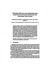
Fig. 2: Average image of 30 healthy fetuses after resizing (Section 2) and alignment defined by anatomical landmarks (Section 2). It highlights the characteristic intensity patterns in fetal MRI for the brain, heart, lungs and liver.

Preprocessing: There is a large variability in the MR scans of fetuses due to fetal development. In particular, the length of the fetus increases by 50% between 23 weeks and term (40 weeks) [2]. We thus propose to normalize the size of all fetuses by resampling the images to an isotropic voxel size sga that is a function of the gestational age (GA), so that a fetus of 30 weeks is resampled to a voxel size s30 : sga = CRLga /CRL30 × s30 , where CRL denotes the crown-rump length [2]. This differs from previously proposed methods which either ignored the GA [1,6,7] or only used it to define size constraints [9]. Moreover, fetal MRI is typically acquired as stacks of 2D images that freeze in-plane motion but form a 3D volume corrupted by fetal and maternal motion. The images are thus preprocessed using median filtering to attenuate motion artifacts. Detecting candidate locations for the heart: In theory, a detector could be trained on aligned images while at test time, it would be applied to all possible rotated versions of the 3D volume. However, in practice it would be too time consuming to explore an exhaustive set of rotations. In particular, the integral image that is used to extract intensity features would need to be computed for all tested rotations. Instead of rotating the image itself, we thus propose to rotate the sampling grid of the image features. This is done by defining a local orientation of the 3D volume for every voxel. When training the classifier, all voxels are oriented using the anatomy of the fetus (Fig. 2 and Fig. 3.a): ~u0 points from the heart to the brain, ~v0 from the left lung to the right lung and w ~ 0 from back to front (w ~ 0 = ~u0 × ~v0 ). When applying the detector to a new image, in theory, all possible orientations (~u, ~v , w) ~ should be explored. However, assuming that the location of the brain is already known [9], ~u can be defined as pointing from the current voxel x to the brain (Fig. 3.b). In this case, only the orientation of the plane Px,~u passing through x and orthogonal to ~u remains undefined. (~v , w) ~ are then randomly chosen so that they form an orthonormal basis of Px,~u . The rationale for this definition of ~u is that when x is positioned at the center of the heart, Px,~u is the transverse plane of the fetal anatomy (Fig. 2). To address the sensitivity to the brain localization, a random offset is added to the estimated brain center with a 10mm range comparable to the prediction errors reported in [9]. Additionally, knowing the location of the

4

K. Keraudren et al.

~v ~v0

~v0

~u

~u0

~u

~u0

~v0

~u0

~v

~u ~v

(a)

(b)

Fig. 3: (a) When training the classifier, features (light blue squares) are extracted in the anatomical orientation of the fetus: ~u0 points from the heart (green) to the brain (red ), and ~v0 points from the left lung (blue) to the right lung (yellow ). The pink contour corresponds to the liver. (b) At testing time, features are extracted in a coordinate system rotating around the brain. brain, the search for the heart only needs to explore the image region contained between two spheres of radii R1 and R2 (Fig. 4) that are independent of the GA thanks to the size normalization. The localization of the heart is performed in two stages: a classification forest is first applied to obtain for each voxel x a probability p(x) of being inside the heart (Fig 5.a). All voxels with p(x) > 0.5 are then passed on to a regression forest, which predicts for each of them the offset to the center of the heart. Using the predicted offsets, the probabilities are then accumulated in a voting process, and the voxels receiving the highest sum of probabilities are considered as candidate centers for the heart (Fig 5.b). During classification, in order to increase the number of true positives, an initial random orientation of the plane Px,~u is chosen and the detector is successively applied by rotating (~v , w) ~ with an angular step θ. The value of (~v , w) ~ maximizing the probability of the current voxel to be inside the heart is selected, and only this orientation of Px,~u is passed on to the regression step. Four types of features are used in the RFs: tests on image intensity, gradient magnitude, gradient orientation and distance from the current voxel to the brain. In order to be invariant to intensity shifts [10], image intensity or gradient magnitude features select two axis-aligned cube patches of random sizes at random offsets from the current voxel and compare their mean intensity. All features are extracted in the local orientation (~u, ~v , w). ~ Similarly, during the voting process, the predicted offsets are computed with the same local orientation. Detecting candidate locations for the lungs and liver: For each candidate location of the heart, candidate centers for the lungs and liver are detected. Similarly to the heart detection, a classification RF first classifies each voxel as either heart, left lung, right lung, liver or background. For each organ, a

Automated Localization of Fetal Organs in MRI

R

3

R1

5

R2

Fig. 4: Knowing the location of the brain, the search for the heart can be restricted to a narrow band within two spheres of radius R1 and R2 (red ). Similarly, knowing the location of the heart, the search for the lungs and the liver can be restricted to a sphere of radius R3 (green).

regression RF is then used to vote for the organ center. During training, the images are oriented according to the fetal anatomy (Fig. 2). During testing, both the location of the brain and heart are known and only the rotation around the heart-brain axis needs to be explored. For each voxel x, we can hence set ~u = ~u0 , and only the orientation of the plane Px,~u0 remains unknown. (~v , w) ~ are thus randomly chosen to form an orthonormal basis of Px,~u0 . In the set of features for the RFs, the distance from the current voxel to the brain, which was used in the detection of the heart, is now replaced by the distance to the heart. Additionally, the projection of the current voxel on the heart-brain axis is used in order to characterize whether the current voxel is below or above the heart relative to the brain. Similarly to the heart detection, the detector is run with an angular step θ. For each voxel, the value of θ maximizing the probability of being inside one of the organs of the fetus is selected. Spatial optimization of candidate organ centers: The voting results from the regression RF are first smoothed with a Gaussian kernel. Local maxima are then extracted to form a set of candidates xl for the center of each organ, l ∈ L = { heart, left lung, right lung, liver }, along with their individual scores p(xl ). Each combination of candidate centers is assigned a score (Eq. 1) based on the individual scores p(xl ) and the spatial configuration of all organs: X

1

λp(xl ) + (1 − λ)e− 2 (xl −¯xl )

>

Σl−1 (xl −¯ xl )

(1)

l∈L

where x ¯l is the mean position and Σl the covariance matrix for the organ l in the training dataset, computed in the anatomical coordinate system of the fetus. λ is a weight between individual scores and the spatial configuration of organs. Once the organ centers have been localized, the voting process can be reversed in order to obtain a rough segmentation (Fig. 5.c).

6

K. Keraudren et al.

(a)

(b)

(c)

Fig. 5: (a) Probability of a voxel to be inside the heart. (b) Accumulated regression votes for the center of the heart. (c) After all organs have been located, the voting process can be reversed, resulting in a rough segmentation for each organ: heart (blue), left lung (red ), right lung (green), liver (yellow ).

3

Experiments

Datasets: Two datasets of 1.5T T2-weighted ssTSE images were used in this paper. The first dataset was used to train and validate the model in a leaveone-out cross validation, in the absence of motion artifacts. It consists of 55 scans covering the whole uterus for 30 healthy subjects and 25 IUGR subjects (scanning parameters: TR 1000ms, TE 98ms, 4mm slice thickness, 0.4mm slice gap). The second dataset is used to test the model in the presence of motion artifacts. There are 224 scans, from 64 healthy subjects, which do not all fully cover the fetal body (scanning parameters: TR 15000ms, TE 160ms, 2.5mm slice thickness, 1.5mm slice overlap). A ground truth segmentation for all fetal organs was provided by an expert for the first dataset. Due to the large number of images and the presence of motion artifacts, only the center of each organ has been manually annotated in the second dataset. The location of the brain is passed to the detector for the first dataset in order to evaluate the proposed method on its own while the method of [9] is used to localize the brain automatically in the second dataset, thus evaluating a fully automated localization of fetal organs. Both datasets cover the range of gestational ages from 20 to 38 weeks. Results: The results are reported as detection rates in Table 1, where a detection is considered successful for the organ l if the predicted center is within the ellipsoid defined by (xl − yl )> Σl−1 (xl − yl ) < 1 where yl is the ground truth center. For the first dataset, Σl is the covariance matrix of the ground truth segmentation while for the second dataset, it is defined from training data as in Section 2. The distance error between the predicted centers and their ground truth are reported in Fig. 6. Although healthy and IUGR subjects were mixed in the training data, results are reported separately to assess the performance of the detector when fetuses are small for their gestational age. Training two detectors on each subset of the data did not improve the results. The higher detection

Automated Localization of Fetal Organs in MRI

7

Table 1: Detection rates for each organs.

st

1 dataset: healthy 1st dataset: IUGR 2nd dataset

Distance error (mm)

40

1st dataset: healthy

Heart

Left lung

Right lung

Liver

90% 92% 83%

97% 60% 78%

97% 80% 83%

90% 76% 67%

40

1st dataset: IUGR

40

35

35

35

30

30

30

25

25

25

20

20

20

15

15

15

10

10

10

5

5

5

0

0

Left Right Heart Liver lung lung

Left Right Heart Liver lung lung

0

2nd dataset

Left Right Heart Liver Brain lung lung

Fig. 6: Distance error between the predicted organ centers and their ground truth for the first dataset (30 healthy fetuses and 25 IUGR fetuses) and the second dataset (64 healthy fetuses).

rate for the lungs than for the heart for the healthy subjects of the first dataset (Table 1) is due to the detector overestimating the size of the heart (Fig 5.c), which can be linked to the signal loss when imaging the fast beating heart. A decrease in performance can be observed for the detection of the lungs in IUGR fetuses, which can be associated with a reduction in lung volume reported in [4]. The asymmetry in the performance of the detector between the left and right lungs can be explained by the presence of the liver below the right lung, leading to a stronger geometric constraint in Eq. 1. For the second dataset, the largest error for the detection of the brain detection using the method of [9] is 21mm, which is inside the brain and is sufficient for the proposed method to succeed. In 90% of cases, the detected heart center is within 10mm of the ground truth, which suggests that the proposed method could be used to provide an automated initialization for the motion correction of the chest [8]. Beside motion artifacts, the main difference between the first and second dataset is that the second dataset does not fully cover the fetal abdomen in all scans, which could explain its lower performance when detecting the liver. Training the detector takes 2h and testing takes 15min on a machine with 24 cores and 128 GB RAM. The parameters in the experiments were chosen as follows: s30 = 1mm, maximal patch size 30 pixels, maximal offset size 20 pixels, λ = 0.5, θ = 90◦ .

8

4

K. Keraudren et al.

Conclusion

We presented a pipeline which, in combination with automated brain detection, enables the automated localization of the lungs, heart and liver in fetal MRI. The localization results can be used to initialize a segmentation or motion correction, as well as to orient the 3D volume with respect to the fetal anatomy to facilitate clinical diagnosis. The key component to our method is to sample the image features in a local coordinate system in order to cope with the unknown orientation of the fetus. During training, this coordinate system is defined by the fetal anatomy while at test time, it is randomly oriented, within constraints set by already detected organs. In future work, the possibility to merge the classification and regression steps into a Hough Forest [5] will be investigated.

References 1. Anquez, J., Angelini, E., Bloch, I.: Automatic Segmentation of Head Structures on Fetal MRI. In: ISBI. pp. 109–112. IEEE (2009) 2. Archie, J.G., Collins, J.S., Lebel, R.R.: Quantitative Standards for Fetal and Neonatal Autopsy. American Journal of Clinical Pathology 126(2), 256–265 (2006) 3. Breiman, L.: Random Forests. Machine learning 45(1), 5–32 (2001) 4. Damodaram, M., Story, L., Eixarch, E., Patkee, P., Patel, A., Kumar, S., Rutherford, M.: Foetal Volumetry using Magnetic Resonance Imaging in Intrauterine Growth Restriction. Early Human Development (2012) 5. Gall, J., Lempitsky, V.: Class-specific Hough Forests for Object Detection. In: CVPR. pp. 1022–1029. IEEE (2009) 6. Ison, M., Donner, R., Dittrich, E., Kasprian, G., Prayer, D., Langs, G.: Fully Automated Brain Extraction and Orientation in Raw Fetal MRI. In: Workshop on Paediatric and Perinatal Imaging, MICCAI. pp. 17–24. Springer (2012) 7. Kainz, B., Keraudren, K., Kyriakopoulou, V., Rutherford, M., Hajnal, J.V., Rueckert, D.: Fast Fully Automatic Brain Detection in Fetal MRI using Dense Rotation Invariant Image Descriptors. In: ISBI. pp. 1230–1233. IEEE (2014) 8. Kainz, B., Malamateniou, C., Murgasova, M., Keraudren, K., Rutherford, M., Hajnal, J., Rueckert, D.: Motion Corrected 3D Reconstruction of the Fetal Thorax from Prenatal MRI. In: Golland, P., Hata, N., Barillot, C., Hornegger, J., Howe, R. (eds.) MICCAI 2014, part II, LNCS, vol. 8674, pp. 284–291. Springer, Heidelberg (2014) 9. Keraudren, K., Kyriakopoulou, V., Rutherford, M., Hajnal, J.V., Rueckert, D.: Localisation of the Brain in Fetal MRI Using Bundled SIFT Features. In: Mori, K., Sakuma, I., Sato, Y., Barillot, C., Navab, N. (eds.) MICCAI 2013, part I, LNCS, vol. 8149, pp. 582–589. Springer, Heidelberg (2013) 10. Pauly, O., Glocker, B., Criminisi, A., Mateus, D., M¨ oller, A., Nekolla, S., Navab, N.: Fast Multiple Organ Detection and Localization in Whole-Body MR Dixon Sequences. In: Fichtinger, G., Martel, A., Peters, T. (eds.) MICCAI 2011, part III, LNCS, vol. 6893, pp. 239–247. Springer, Heidelberg (2011) 11. Pedregosa, F., et al.: Scikit-learn: Machine Learning in Python. Journal of Machine Learning Research 12, 2825–2830 (2011) 12. Zheng, Y., Barbu, A., Georgescu, B., Scheuering, M., Comaniciu, D.: Fast Automatic Heart Chamber Segmentation from 3D CT Data using Marginal Space Learning and Steerable Features. In: ICCV. pp. 1–8. IEEE (2007)