Automatic and Precise Orthorectification, Coregistration, and Subpixel

IEEE TRANSACTIONS ON GEOSCIENCE AND REMOTE SENSING, VOL. 45, NO. 6, JUNE 2007

1529

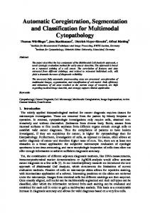
Automatic and Precise Orthorectification, Coregistration, and Subpixel Correlation of Satellite Images, Application to Ground Deformation Measurements Sébastien Leprince, Student Member, IEEE, Sylvain Barbot, Student Member, IEEE, François Ayoub, and Jean-Philippe Avouac

Abstract—We describe a procedure to accurately measure ground deformations from optical satellite images. Precise orthorectification is obtained owing to an optimized model of the imaging system, where look directions are linearly corrected to compensate for attitude drifts, and sensor orientation uncertainties are accounted for. We introduce a new computation of the inverse projection matrices for which a rigorous resampling is proposed. The irregular resampling problem is explicitly addressed to avoid introducing aliasing in the ortho-rectified images. Image registration and correlation is achieved with a new iterative unbiased processor that estimates the phase plane in the Fourier domain for subpixel shift detection. Without using supplementary data, raw images are wrapped onto the digital elevation model and coregistered with a 1/50 pixel accuracy. The procedure applies to images from any pushbroom imaging system. We analyze its performance using Satellite pour l’Observation de la Terre (SPOT) images in the case of a null test (no coseismic deformation) and in the case of large coseismic deformations due to the Mw 7.1 Hector Mine, California, earthquake of 1999. The proposed technique would also allow precise coregistration of images for the measurement of surface displacements due to ice-flow or geomorphic processes, or for any other change detection applications. A complete software package, the Coregistration of Optically Sensed Images and Correlation, is available for download from the Caltech Tectonics Observatory website. Index Terms—Change detection, coseismic displacements, geocoding, image registration, image resampling, optical imagery, orthorectification, Satellite pour l’Observation de la Terre (SPOT), satellites, subpixel correlation.

I. I NTRODUCTION

E

ARTH SURFACE changes can be determined by comparing pairs of optical satellite images acquired on different

Manuscript received April 28, 2006; revised October 25, 2006. This work was supported in part by the National Science Foundation Grants EAR-0409652 and EAR-0636097 and by the Gordon and Betty Moore Foundation. This is Caltech Tectonics Observatory contribution #52. S. Leprince is with the Department of Electrical Engineering, California Institute of Technology, Pasadena, CA 91125 USA (e-mail: leprincs@ caltech.edu). S. Barbot was with the Division of Geological and Planetary Sciences, California Institute of Technology, Pasadena, CA 91125 USA. He is now with the Institute of Geophysics and Planetary Sciences, Scripps Institution of Oceanography, University of California, San Diego, La Jolla, CA 92093 USA. F. Ayoub and J.-P. Avouac are with the Division of Geological and Planetary Sciences, California Institute of Technology, Pasadena, CA 91125 USA. Digital Object Identifier 10.1109/TGRS.2006.888937

dates. Precise images coregistration is a prerequisite in such applications, and this critical step is often a major source of limitation [1], [2]. For instance, a registration accuracy of less than 1/5 of a pixel is required to achieve a change detection error of less than 10% in Landsat Thematic Mapper images [3]. As to the measurement of Earth surface displacements, which is the driving motivation of this paper, most applications require a measurement accuracy of less than 1 m. This implies that the images co-registration accuracy should be even less, i.e., significantly smaller than the pixel size of most currently available optical satellite images. Examples of such applications include the measurement of coseismic ground deformations [4]–[7], ice flow [8], and sand dune migrations [9]. Difficulties in accurately coregistering satellite images arise from the nonideal characteristics of the optical systems, the changing attitude of the spacecraft during the scanning operation of the images, digital elevation model (DEM) errors, and inaccurate resampling. The accuracy of the measurements of ground displacements, in addition, depends on the performance of the correlation technique. Despite these difficulties, encouraging results were obtained in a number of studies. It should be noted, however, that they were all carried on using data from only one imaging system and under restrictive conditions such as similar viewing angles and satellite tracks [4], [10], [11] or using external information from global positioning system (GPS) measurements [6]. Precise coregistration of images with viewing angle differing by more than 3◦ also seems out of reach [4], [11]. The operational use of such a technique, in particular to monitor coseismic deformations, would benefit from a more generic approach, allowing to cross-correlate images from different imaging systems with different viewing angles, and without the need for information other than what is extracted from the satellite ancillary data and the topography. To be coregistered, remotely sensed images need to be projected and resampled onto some common reference system. One method consists of fixing one image as the reference image, the master image. Its viewing geometry defines the common reference system, and other images, the slave images, are projected and resampled onto this reference system. Analysis of images’ discrepancies is carried out in this reference frame by applying the desired change detection algorithm. This approach is commonly used in processing pairs of radar images

0196-2892/$25.00 © 2007 IEEE

1530


to produce differential interferograms [12]. Examples with optical images are found in [5] and [8]. A second method is to project and resample each image onto a reference system that is independent of the satellite viewing geometry, such as a ground projection. The technique, thus, consists of projecting images onto the ground according to their viewing geometry, with the change detection analysis being performed on the set of ground images generated. This approach is illustrated in [4], [6], and [7]. Here, we prefer this second method. It is the most flexible way to coregister images from different acquisition systems (e.g., pushbroom images, aerial photographs, etc.), and the production of ground-projected images provides a georeferenced by-product suitable for many other needs. This paper describes an automatic processing chain to accurately and rigorously coregister and compare a set of optical satellite images. The processing chain is composed of four fundamental processes: The first process projects each pixel from the satellite focal plane onto a ground reference system. This operation utilizes knowledge from both the imaging system and the ground topography. The second process performs the resampling of the acquired image according to the projection mapping previously calculated. This yields ground-projected images, called ortho-rectified images. Cumulative uncertainties on both the imaging system and the topography lead to distortions and misregistrations between the pairs of orthorectified images to be compared. The processing chain is therefore augmented with a third process, optimizing the satellite viewing parameters with respect to some reference frame. This reference frame will be either a shaded version of the topography model or another image previously ortho-rectified. Misregistrations to be corrected are measured from the fourth process, a correlation. In this paper, we focus on images from the Satellite pour l’Observation de la Terre (SPOT) satellite systems principally because raw images are delivered with all the acquisition parameters [ephemeris, attitude components during the imaging process, charge coupled device (CCD) look directions, etc.] provided in ancillary data [13]. We also use panchromatic (PAN) images rather than multispectral images because of their higher ground resolution, which is a major advantage for the measurement of ground deformations. PAN images of the SPOT satellites 1, 2, 3, and 4 have a ground resolution of 10 m. The 5- and 2.5-m ground resolutions are available from SPOT 5. The technique presented can be applied to any multispectral images, making it appropriate for any change detection applications. Images from other pushbroom systems also can be processed from our methodology, as explained for Advanced Spaceborne Thermal Emission and Reflection Radiometer (ASTER) images in Appendix IV. An application is given by the study in [14]. The first three sections of this paper present, respectively, the orthorectification mapping computation, the resampling scheme, and the correlation-registration algorithm. The fourth section describes the global optimization mechanism and the processing chain that allows for accurate images orthorectification and coregistration. Finally, the last section assesses the quality of the whole process and presents an application to the measurement of a coseismic displacement field.

II. P USHBROOM G EOMETRY AND O RTHORECTIFICATION M ODELS A rigorous way to register satellite images is to determine the orthorectification parameters for each image such that precise registration is achieved. We therefore first examine the modeling of the SPOT satellites viewing geometry. SPOT satellites are pushbroom imaging systems, meaning that all optical parts remain fixed during the images acquisition and the scanning is accomplished by the forward motion of the spacecraft. Each line in the image is then acquired at a different time and submitted to the variations of the platform. Since the pushbroom acquisition system of all SPOT satellites are modeled by the same set of equations (see Appendix IV for the case of ASTER images), it is possible to derive a common orthorectification scheme. A. Direct Orthorectification Model The direct orthorectification model computes the geographic location on the ground where each pixel in the raw image, i.e., the focal plane of the instrument, has to be projected. Notations are derived from the SPOT satellite geometry handbook [15]. 1) Navigation Reference Coordinate System and Look Directions: The navigation reference coordinate system (O1 , X1 , Y1 , Z1 ) is the spacecraft body fixed reference system. O1 is the satellite center of mass and denoting the satellite , the axes are defined position and velocity vectors by P and V such that, at nominal attitude when the satellite roll, pitch and yaw are null angles, we have  1 //V Y 1 //P Z  1 = Y 1 ∧ Z 1. X

(1)

The SPOT satellites (1, 2, 3, 4, and 5) positions and velocities are given in Cartesian coordinates with reference to the International Terrestrial Reference Frame (ITRF) [16]. In the past years, the WGS 84 geodetic system has been gradually aligned to the successive ITRF realizations. For this paper, we can consider that the WGS 84 and the different ITRF realizations are undistinguishable, and we then express all coordinates in the WGS 84 reference system. The SPOT satellites sensor consists of a CCD line array responsible for the image pushbroom scanning operation. Expressed in the navigation reference coordinate system, the look directions are modeling the equivalent pointing direction of each CCD element. By being constant during the image acquisition, they provide the internal camera model accounting for the mirror rotation, optical distortions, and calibration parameters resulting from on-ground postprocessing. The look directions are provided in ancillary data in the form of a two angle rotation (Ψx , Ψy ) around the satellite body fixed system axes (Fig. 1). Hence, for all columns c and for all rows r in the raw image, the look directions u1 are given by u1 (c, r) =

u1 (c, r) , u1 (c, r)2

for all c, r = 1, . . . , N

(2)

LEPRINCE et al.: ORTHORECTIFICATION, COREGISTRATION, AND SUBPIXEL CORRELATION

1531

Fig. 1. Definition of the look direction u1 from the look angles Ψx and Ψy in the navigation reference coordinate system.

with



 − tan Ψy (c) u1 (c, r) =  tan Ψx (c)  , −1

Fig. 2. Orbital coordinate system and attitude variations.

for all r



where N is the number of CCD elements in the line array. Theoretically, these look directions should be attached to the optical center of the imaging system. Here, we assume that they are attached to the center of mass O1 , since to our knowledge, no model linking the optical center to the center of mass is available. However, the nonlinear distortions induced by this approximation account for much less than a millimeter on the ground and are neglected here. Furthermore, the static error is absorbed from the parameters optimization (Section V-A2). 2) Orbital Coordinate System and Attitude Variations: The orbital coordinate system (O2 , X2 , Y2 , Z2 ) is centered on the satellite (O2 = O1 ), and its orientation is based on the spacecraft position in space (Fig. 2). Roll, pitch, and yaw variations are given as rotation angles around the Y2 , X2 , and Z2 axes defined by  2 (t) = P (t)  Z   P (t)2  (3) 2 (t) = V (t)∧Z 2 (t) X  V (t)∧Z 2 (t)2    2 (t) = Z 2 (t) ∧ X 2 (t) Y (t) are the instantaneous position and velocwhere P (t) and V ity of the satellite, respectively. For historical reasons, SPOT attitudes data are expressed within the inverted navigation reference coordinate system [15]. Applying this convention and given ap (t), ar (t), and ay (t), which are the absolute rotation angles around the pitch, roll, and yaw axes at time t, respectively, the satellite look directions u2 (c, r) in the orbital coordinate system for all CCD elements are given, for all c, r = 1, . . . , N , by u2 (c, r) = Rp (r) · Rr (r) · Ry (r) · u1 (c) with



1 Rp (r) =  0 0

0 cos ap (r) − sin ap (r)



0 sin ap (r)  cosp (r)

(4)

 cos ar (r) 0 − sin ar (r)  Rr (r) =  0 1 0 sin ar (r) 0 cos ar (r)   cos ay (r) − sin ay (r) 0 Ry (r) =  sin ay (r) cos ay (r) 0  0 0 1 where Rr (r), Rp (r), and Ry (r) are the roll, pitch, and yaw rotation matrices at the time of acquisition of image row r. 3) Look Directions in Terrestrial Coordinate System: For each pixel in the raw image, the corresponding look direction u3 expressed within the terrestrial coordinate system is then   X2x (r) Y2x (r) Z2x (r) u3 (c, r) =  X2y (r) Y2y (r) Z2y (r)  · u2 (c, r). (5) X2z (r) Y2z (r) Z2z (r) 4) Location on Earth Model: The corresponding ground location M of the raw image pixel (c, r) is determined by calculating the intersection between u3 (c, r) and the Earth ellipsoid model. For any of such pixel, we are then to find the point M (xM , yM , zM ) that verifies −−→ −−−→ O3 M (c, r) = O3 P (r) + µ.u3 (c, r), for µ > 0 and

x2 + y 2 z2 A=a+h + = 1, with B =b+h A2 B2

(6)

where O3 is the Earth Cartesian center and a and b are, respectively, the semimajor and semiminor axis of the ellipsoid. h is the approximated elevation above the ellipsoid at the ground location M . For any pixel (c, r), µ is determined such that 2 Px u3 +Py u3 u3x +u23y 2 u23z P u x y + zB 23z µ + B2 µ + 2 A2 A2 2 2 Pz2 = 1 y + PxA+P +B 2 2 −−→ where O3 P (r) = (Px , Py , Pz ) and u3 (c, r) = (u3x , u3y , u3z ). The smallest solution µ1 is to be kept (the largest one intersecting with the other side of the ellipsoid) and used in (6) to obtain the geocentric coordinates M (xM , yM , zM ) of the pixel (c, r).

1532


Using a DEM, the intersection with the topographic surface is computed by locally and successively approximating the topography with a wider ellipsoid (Appendix I). 5) Direct Model Transformation Matrices: All the pixels in the raw image are associated with Cartesian geocentric coordinates, which can be converted into geodetic coordinates and then into Universal Transverse Mercator (UTM) coordinates [17], expressed in meters, like the ground displacements to be measured. These ground coordinates are stored in two matrices N and E representing the Northing and Easting components. The pixel of coordinates (c, r) in the raw image will then have the ground coordinates {E(c, r), N (c, r)}. The transformation matrices provide necessary information to resample the raw image and to produce an ortho-rectified image. However, this approach contains an important drawback: It projects the regular pixel grid from the instrument focal plane to an irregular grid on the ground. On a large scale, irregularities result from the global rotation between the raw and ortho-rectified images due to the satellite orbit inclination. On a more local scale, irregularities are due to changing in the satellite attitudes and to the topography roughness. For specific applications in seismotectonics, coseismic displacements are typically of a subpixel scale. The resampling of the images therefore needs particular attention to preserve subpixel information from the raw images; resampled images have to respect the Shannon–Nyquist sampling criterion to avoid aliasing (Section III-A). B. Inverse Orthorectification Model To allow for the rigorous resampling of the images to orthorectify, we determine the noninteger pixel coordinates in the raw image of a predefined regular grid on the ground. This operation, called the inverse orthorectification model, has been investigated in several studies [18]–[20]. However, they are all based on the collinearity equations stating that a point in the focal plane, the optical center, and the imaged point on the ground are all aligned. This assumption is no longer valid in the presence of aberrations or distortions from the imaging system. Modern satellites, such as SPOT satellites, provide look directions as a complete physical model of the imaging system [15]. We therefore propose a new inverse orthorectification scheme, which fully exploits the information from the ancillary data, by inverting the direct orthorectification model. Our scheme assumes that any given point on the ground lying inside or in the close vicinity of the imaged area has one and only one corresponding point in the image plane or in its close vicinity. We extend the assumption to the close vicinity of the image because we extrapolate attitude and sensor values outside the image plane. In practice, this assumption is satisfied when dealing with a stable imaging system and can be verified a posteriori. We have never encountered limitations due to this assumption. 1) Orthorectification Grid: To compare a set of coregistered images, all images have to be rectified onto a common grid. The orthorectification grid is therefore defined as the smallest rectangular grid that includes the image footprint and whose starting coordinates (UTM) are multiple of the desired image

Fig. 3.

Inverse orthorectification model principle.

resolution. Comparable images (ortho-rectified at the same resolution) will then not suffer from grid misalignment. The image footprint is determined by application of the direct orthorectification model to the four corners of the raw image. 2) Inverse Orthorectification Principle: Given a point M on the ground (on the orthorectification grid), its elevation is determined from bicubic interpolation of the DEM, and its coordinates converted into the Earth centered Cartesian WGS 84 system [17]. Equation (5) gives the look directions u3 (c, r) for all c, r = 1, . . . , N . Now, we consider a continuous version of the look directions with the notation u3 (x, y) and (x, y) ∈ R2 . Finding the pixel coordinates (x, y) in the raw image that are associated with a given point M (xM , yM , zM ) on the ground is equivalent to finding (x, y) ∈ R2 that minimize the function 2 −−−→ −−−→ Φ(x, y) = O3 M − O3 M (x, y) (7) 2

where M (x, y) should be the point on the ground seen from −−→ the look direction u3 (x, y). Let O3 P = (Px , Py , Pz ) be the satellite position for the look angle u3 . Assuming a rectilinear propagation of light through the atmosphere, the line of sight −−→ implied by u3 = (u3x , u3y , u3z ) is s = O3 P + t · u3 , for some t > 0. If M lies at the intersection between s and the topography, determining its coordinates is extremely tedious, and the nonlinearities of the topography may cause the minimization of Φ to fail. For both simplicity and efficiency, we construct a projection plane for each point M on the orthorectification grid, on which M actually lies. The projection plane P(M ) is the −−−→ plane passing through M and perpendicular to O3 M (Fig. 3). Since M ∈ P(M ), the solution of the minimization of Φ is unchanged, but the straightforward computation of M and the near-quadratic regularity of Φ are now ensured. All points −−−→ −−−→ M (α, β, γ) in P(M ) must satisfy O3 M · M M = 0. Hence, the projection plane is explicitly defined by 2 2 xM α + yM β + zM γ − x2M + yM = 0. (8) + zM s then intersects P(M ) for t = t∗ =

d − xM Px − yM Py − zM Pz xM u3x + yM u3y + zM u3z

(9)


1533

with 2 2 d = x2M + yM + zM .

The solution of the inverse orthorectification problem (x∗ , y ∗ ) is therefore obtained by minimizing the function 2 −−−→ −−−→ Φ(x, y) = O3 M − O3 M (x, y) (10)

Fig. 4. General regular resampling scheme.

2

with −−−→ −−→ O3 M (x, y) = O3 P (y) + t∗ · u3 (x, y)

(11)

for all points M in the orthorectification grid. 3) Minimizing Φ: By projecting M onto the plane surface P(M ), the nonlinearities of Φ are now only due to the satellite optical distortions and changing attitudes, which are smoothly varying in the vicinity of the solution. The problem of minimizing Φ is then quasi-linear, and the near-quadratic regularity of Φ makes an unconstrained gradient minimization approach appropriate. The algorithm requires that Φ be a continuous function for all x, y ∈ R, while it is only given at integer pixel locations. Satellite velocities, positions, attitudes, and sensor orientations are then linearly interpolated between pixels and linearly extrapolated beyond the image limits (to satisfy the unconstrained minimization process). The linear extrapolation should preserve the continuity of the values as well as the global motion of the satellite. We have chosen extrapolated points to lie on the line joining the values at the image limits in both x and y directions. Several classical gradient minimization procedures were tested, namely the quasi-Newton, the steepest descent, or the conjugate gradients algorithms, but we occasionally experienced convergence problems when the initialization guess was not accurate. The two-point step size (TPSS) gradient algorithm [21] proved to be more robust and efficient. Implementation details are provided in Appendix II. 4) Inverse Model Transformation Matrices: Outputs of the minimization are stored into two matrices with dimensions determined by the orthorectification grid. x∗ values are stored in the X matrix and y ∗ values in the Y matrix. If the ground coordinates of the upper-left-corner grid element are (E0 , N0 ) and the grid resolution is r, then at the ground location (E0 + i · r, N0 − j · r), the pixel of coordinates (X(i, j), Y (i, j)) in the raw image has to be projected. This inverse orthorectification model is used next to resample raw images and to produce precise ortho-rectified images. III. I MAGE R ESAMPLING In the image processing literature the nearest neighborhood, bilinear and bicubic resampling methods are the most commonly used [22]. These methods have been designed with the constraint of keeping a small kernel size to minimize the computational cost inherent to any convolution process. These resampling methods can be seen as a zeroth-, first-, and thirdorder polynomial approximations of the theoretical resampling kernel, the sinc function. Unlike the sinc function, approximating kernels introduce a certain amount of aliasing in the

resampled images [22], which may reduce the accuracy of any correlation process, hence any registration process. For example, it has been observed systematic correlation biases when images were resampled from these methods [4]. Moreover, it will be shown next that an explicit formulation of the irregular resampling problem is required to avoid addition of aliasing while constructing ortho-rectified images. A. Resampling Regularly Spaced Data: Changing the Sampling Rate Consider the continuous band-limited low-pass signal xc (t) sampled at the Nyquist rate 2π/T0 (with T0 as the sampling period). The sampled signal is called xsT0 (t). Resampling a given sampled signal can be done by sampling its reconstructed continuous version at a new rate 2π/T1 . If T1 > T0 , appropriate low-pass filtering of the reconstructed signal, which is equivalent to reconstructing a lower band-limited version of xc (t), is needed to avoid aliasing in the resampled signal xsT1 (t). From the Shannon–Nyquist sampling theorem [23], a general ideal reconstruction filter is written as sin( πt d ) , for t = 0 πt hrd (t) = (12) d 1, for t = 0 where d can be seen as the effective reconstruction period. A general resampling scheme that allows for up-sampling as well as for down-sampling regularly spaced data is designed by setting the parameter d = Max(T0 , T1 ) (Fig. 4). It is to note that up-sampling does not add information and that xsT1 (t) is then oversampled. B. Resampling Irregularly Spaced Data We present an aliasing-free resampling scheme for irregularly spaced data, meaning that either the original sampled signal is irregularly sampled and has to be regularly resampled or the original signal is regularly sampled and has to be irregularly resampled, or any combination of both situations. For simplification, we assume that sampling irregularities account for a small fraction of the mean sampling period. Denote by {T0 } the set of sampling periods of the signal to be resampled and by {T1 } the set of sampling periods of the resampled signal. It is supposed that µ({Ti }) σ({Ti }), for i = 0, 1. Here, µ(·) represents the mean operator and σ(·) the standard deviation operator. µ({Ti }) = Ti and σ({Ti }) = 0 for regularly sampled signals. Therefore, the parameter d of a general reconstruction filter for irregularly spaced data is such that d = max ({T0 }, {T1 }) .

(13)

1534


This ensures that the resampled signal is aliasing free. However, it is locally subjected to oversampling since this scheme is equivalent to reconstructing the signal at its lower regularly sampled resolution. As it will be shown later, this nonoptimality is not a problem for most applications. 1) 2-D Resampling Kernel: For simplicity and computational efficiency, we concentrate on separable resampling kernels. The reconstruction filter is an ideal low-pass filter of the form sin πy sin( πx d dx ) · πy y , for x, y = 0 πx (x, y) = h rdx ,dy

1,

dx

dy

for x, y = 0

where dx and dy are called the “resampling distances.” They represent the maximum distance between adjacent samples in the x and y directions. Practically, a finite length approximation is derived from weighting by a nonrectangular window that tapers close to the edges, the Kaiser window. This helps minimizing the maximum reconstruction error [23] that mostly manifests itself as ringing in the reconstructed image (Gibbs phenomenon). By setting the kernel length to 2N + 1 samples, the 2-D separable Kaiser window is defined by wKdx ,dy (xn , yn )  1 2  I0 βx 1−( Nxdnx ) 2      I0 (βx )  2 12 = I0 βy 1− Nydny    · ,   I0 (βy )   0,

raw image onto the ground at locations that do not belong to a regular grid. According to the previous notations, the signal xsT0 is then irregularly sampled, and we are seeking a way to resample it, yielding xsT1 , which is regularly sampled on the ground. Here, T0 and T1 are sampling periods expressed in geographical units (meters if the UTM projection is chosen). Resampling distances dx and dy are obtained from the maximum absolute differences between adjacent entries in, respectively, the E and N direct transformation matrices. Denote by di,jE and di,jN the local direct resampling distances, taken over eight neighbors, such that

−N dx ≤ xn ≤ N dx −N dy ≤ yn ≤ N dy otherwise for

where I0 (·) represents the zeroth-order modified Bessel function of the first kind and β the shape parameter. Practically, the shape parameters are set to βx = βy = 3 and N = 12 samples. This set up is a reasonable compromise between the meansquare reconstruction error measured on a set of SPOT images and the computational cost. If we call i0 as the image to be resampled and i1 as the resampled image, then i1 is obtained by the following 2-D discrete convolution: 1 i0 [xn , yn ] i1 [x, y] = c(x, y)

di,jE = max (|E(i, j) − E(i ± 1, j ± 1)|) di,jN = max (|N (i, j) − N (i ± 1, j ± 1)|)

for all entries (i, j) of the direct transformation matrices. If the ortho-rectified grid resolution is given by Rx in the east/west direction and by Ry in the north/south direction, the global resampling distances are given by

(14)

d = max (T0 , {T1 }) .

(16)

If we denote by di,jx the local distances of the X matrix, then  |Xi,j − Xi−1,j−1 |, |Xi,j − Xi,j−1 |  |X − Xi−1,j |, |Xi,j − Xi+1,j−1 |  = max  i,j  |Xi,j − Xi+1,j+1 |, |Xi,j − Xi,j+1 | |Xi,j − Xi−1,j+1 |, |Xi,j − Xi+1,j | 

with c(x, y) =

(15)

over all local resampling distances. However, difficulties in applying the general resampling scheme described in Section III-A arise from the computation of the discrete convolution. The convolution is indeed to be performed on the ground-projected pixels. For each pixel of the ortho-rectified image, projected raw pixels falling within the resampling kernel extent, given by Dx and Dy in (14), have to be determined. A search in the direct transformation matrices is then needed for all points to be resampled, leading to a computationally inefficient scheme [19]. It is also non-rigorous since the resampling kernel cannot be discretized regularly; its discretization depends on the raw pixels projection. 3) Resampling Using Inverse Transformation Matrices: The inverse transformation matrices map a regular grid on the ground onto an irregular grid in the raw image. This is equivalent to considering {T0 } = {1} (raw image sampled at every pixels) regular and {T1 } irregular, with both expressed in pixels since they are defined in the raw image space. We define dx and dy , which must each verify

xn ∈Dx yn ∈Dy

×hrdx ,dy (x − xn , y − yn )wKdx ,dy (x − xn , y − yn )

dx = max ({di,jE } , Rx ) dy = max ({di,jN } , Ry )

xn ∈Dx yn ∈Dy

hrdx ,dy (x − xn , y − yn ) × wKdx ,dy (x − xn , y − yn )

where Dx = [x − N dx , x + N dx ] and Dy = [y − N dy , y + N dy ]; {xn , yn } are the original data samples and {x, y} are the resampled data points. 2) Resampling Using Direct Transformation Matrices: The direct transformation matrices allow to project pixels of the

di,jx

(17)

for all points (i, j) in the matrix X whose coordinates X(i ± 1, j ± 1) are within the raw image. Then, to avoid aliasing, one should choose dx = max(1, max({di,jx })). dy is determined using the same procedure applied to the Y matrix. Resampling is now straightforward because the points to be resampled are defined within the regular dataset of the raw image.


4) Direct and Inverse Resampling Differences: From (15), we notice that there exists a ground resolution (Rx , Ry ) beyond which the resampling distances of the direct scheme will everywhere be (Rx , Ry ). The irregularities in the resampling distances are smaller than the nominal ground resolution of the image σ({Ti }) µ({Ti }); then in the case of a direct resampling scheme, if images are resampled at half their nominal resolution or lower, the resampling distances will always equal the ortho-rectified grid resolution. With the inverse model procedure, since the resampling points are only computed at the ortho-rectified grid resolution, the resampling distances will always be subjected to irregularities. Concretely, if the satellite nominal resolution is 10 m and a 20-m ortho-rectified image is constructed, it will lead to dx = dy = 20 m when resampling with the direct scheme and to dx > 2 pixels and dy > 2 pixels when resampling with the inverse scheme. The image resampled with the inverse model will contain less high frequencies (due to more oversampling), and the image obtained from the direct model will have a higher effective resolution. This difference does not exist if images are resampled close to their nominal resolution, which is generally the case. It is also minimized if images are resampled lower than half their nominal resolution. The complexity of the direct scheme is therefore not justified.

1535

Fig. 5. Raw image.

Fig. 6. Ortho-rectified image.

C. Inverse Resampling Results We present some results from an image that has been processed using the inverse orthorectification model and the inverse resampling procedure. The raw image is a SPOT 5 PAN image of the Hector Mine area in California with a nominal ground resolution of 5 m, and the scene orientation is 13.6◦ . It is ortho-rectified at a ground resolution of 10 m on a UTM projection. The computed resampling distances are dx = 2.501 pixels and dy = 2.413 pixels. The raw and the ortho-rectified images are presented in Figs. 5 and 6. 1) Resampling Distances: The rescaling factor is 1/2 (the resolution is lowered by a factor of two). The resampling distances should then be dx = dy = 2 pixels. The rotation angle corresponds to the scene orientation α = 13.6◦ . Geometrically, if we take a square of side length a, rotating it by an angle α, then the smallest nonrotated square√ that will contain the rotated one will have a side length d = a 2 cos((π/4) − α). Taking a = 2 pixels, the first-order approximation of the resampling distances is then dx = dy = 2.414 pixels. Accounting for local distortions due to topography and satellite attitude variations, the resampling distances computed from the transformation matrices differ slightly from this estimate. This validates the resampling distance computation. Moreover, this computation is done with no a priori knowledge on the scene orientation, making this resampling scheme suitable for all optical imaging systems. Fig. 7 shows that the irregularities of the sampling periods are much smaller than the average sampling periods, as assumed above. In this particular case, µ({di,jx }) = 2.41 pixels with σ({di,jx }) = 0.020 pixel, and µ({di,jy }) = 2.40 pixels with σ({di,jy }) = 0.036 pixel.

Fig. 7. Distribution of local resampling distances (in pixels) for each transformation matrix.

2) Fourier Spectrum of Ortho-Rectified Images: Figs. 8 and 9 represent the Fourier spectrum of the raw and orthorectified images. These spectrums have been computed over small corresponding areas. The zero frequency is at the center of the images. The rotation seen in the ortho-rectified image spectrum reflects the general rotation applied to the raw image [24] when producing the ortho-rectified image. However, distortions due to the local topography are here producing a shear effect. The truncation of the spectrum is visible since it fits within the bandwidth defined by the Nyquist resampling frequency. As no aliasing (no frequency folding on the edges) is noticed in the ortho-image spectrum, we conclude that resampling distances are correctly computed. The dark areas of the ortho-rectified spectrum denotes oversampling, making this resampling

1536


the resampling grid could be estimated from the local rotations in the inverse transformation matrices. Another improvement would be to use locally adaptive resampling distances. In areas of steep topography, the resampling distances take high values, while lower values correspond to areas of flatter relief. By imposing the maximum resampling distances to be used for the whole image, oversampling is introduced in flatter topography areas, limiting the image effective resolution in those regions. This could be the main limiting sampling efficiency factor with high-resolution images. These possible improvements would ensure the sampling efficiency of the ortho-rectified image to come close to unity.

Fig. 8. Raw image log-spectrum.

IV. C ORRELATION OF O PTICAL I MAGES A. Statement of the Problem

Fig. 9. Ortho-rectified image log-spectrum.

scheme not optimum: Even though the image is being resampled on a 10-m grid, the frequency content is the one of an image that would be “optimally” resampled at a resolution of approximately 12.5 m. An objective sense of “optimal” resampling is defined from the sampling efficiency. Sampling efficiency.: The sampling efficiency η of a sampling scheme that allows no aliasing is defined as the ratio between the area S, support for the information (where the spectrum is not zero) within the Fourier elementary cell, and the area of the Fourier elementary cell. The cell that periodically tiles the Fourier plane of a discrete signal is defined as the Fourier cell. By applying in the Fourier domain the formula we used in Section III-C1 to deduce the smallest size of a square containing a rotated square, the efficiency of the resampling scheme presented is therefore η(α) =

2 cos2

1 π 4

−α

,

π for α ∈ 0, 4

(18)

where α is the scene orientation. Hence, for a general application, η ∈ [1/2, 1], at most. In this particular example, this gives ηSPOT ≈ 0.69 (η is a decreasing function of α). 3) Possible Improvements: The main limitation of this resampling scheme comes from the separability of the kernel. Ideally, the resampling kernel would be locally rotated, so that it would be aligned with the grid defined by the resampling points in the raw image. Consequently, the vanishing high-frequency points in the Fourier spectrum will all correspond to the Nyquist frequency, the spectrum will not be rotated anymore, and the scene orientation will not induce oversampling. The rotation of

We discuss a technique to accurately and robustly measure the relative displacement between two images of the same resolution, one being the shifted version of the other. The problem to solve is an image registration problem [25] that we have chosen to tackle with correlation methods: two similar images are said to be registered when their cross correlation attains its maximum. The relative displacement is then deduced from the position of best registration. The registration/correlation algorithm needs to meet several requirements. 1) We are primarily interested in measuring coseismic displacements from pre- and postearthquake images. For SPOT 1, 2, 3, and 4 images, the finest resolution available is 10 m. Commonly, horizontal coseismic displacements are less than 10 m. The correlation algorithm must then allow for subpixel measurements with an accuracy of a few tens of centimeters. The required accuracy is therefore at least 1/20 of a pixel. 2) During the image coregistration process, correlation is needed to measure the misregistration to be corrected even though it can be large. The correlation should then also give precise measurements at the multipixel scale, typically half the correlation window size. The image coregistration accuracy should be better than the coseismic displacement measurement accuracy. 3) The spatial resolution of the coseismic offset field measured depends on the size of the sliding correlation window. We therefore seek a method that is reliable on small correlation windows, typically 32 × 32 pixels. 4) Correlation should be as insensitive as possible to temporal decorrelations, data quantization, or other noise sources. 5) For general use, the parameters of the algorithm should not depend on the window size. 6) This algorithm has to be general so that it can process any digital images. We saw that the Fourier spectrum of the ortho-rectified images may be quite peculiar. The algorithm should then adapt to any given spectrum. When extending the global coseismic offset measurement technique to other optical devices (other satellite systems or aerial photographs), this correlation scheme should remain valid.


B. Phase Correlation Methods We focus on particular correlation methods, the phase correlation methods, which have already shown good results for similar applications [4], [6], [7], [10]. All phase correlation methods rely on the Fourier shift theorem [23]: The relative displacement between a pair of similar images is retrieved from the phase difference of their Fourier transform. Let i1 and i2 be two images that differ only by a displacement (∆x , ∆y ) such that i2 (x, y) = i1 (x − ∆x , y − ∆y ).

(19)

By denoting by I1 and I2 their Fourier transform, from the Fourier shift theorem, we have the relation I2 (ωx , ωy ) = I1 (ωx , ωy )e−j(ωx ∆x +ωy ∆y )

(20)

where ωx and ωy are the frequency variables in column and row. The normalized cross-spectrum of the images i1 and i2 is then Ci1 i2 (ωx , ωy ) =

I1 (ωx , ωy )I2∗ (ωx , ωy ) = ej(ωx ∆x +ωy ∆y ) |I1 (ωx , ωy )I2∗ (ωx , ωy )| (21)

where ∗ denotes the complex conjugate. The images’ relative displacement can thus be estimated from the 2-D slope of the cross-spectrum’s phase. By applying the inverse Fourier transform F −1 to (21), we have the correlation function

F −1 ej(ωx ∆x +ωy ∆y ) = δ(x + ∆x , y + ∆y ). (22) The images’ relative displacement can then alternatively be estimated from the coordinates of the correlation peak. In case of subpixel displacements, this peak is not a Dirac delta function anymore, but a down-sampled version of a Dirichlet kernel [26]. Further processing is then required to recover the image shift. These approaches show that phase correlation methods fall into two categories. In the first category, the relative images’ shift is recovered by explicitly estimating the linear phase of the images’ cross-spectrum [4], [27], [28]. In the second category, the relative displacement is calculated by determining the exact location of the correlation peak [26]. In [26], images to be correlated are supposed to be sampled with a sampling efficiency η = 1. This is generally not the case when images have been resampled for orthorectification. Also, to avoid correlation bias, frequency masking should be applied to only select parts of the cross-spectrum where the phase information is valid (images may be corrupted by aliasing or optical aberrations). For these reasons, a correlation algorithm whose main scheme belongs to the first category will be described, adaptive masking being applied on the cross-spectrum. C. Phase Correlation Properties We review some properties of the phase correlation methods and evaluate the sensitivity to additive white noise and blur,

1537

which are two common phenomena [29]. We also discuss the range of measurable image shifts. 1) Image Blur: The image i1 of a natural scene u1 , acquired by an imaging device using incoherent illumination, is modeled as i1 (x, y) = u1 (x, y) ∗ |h1 (x, y)|2

(23)

where h1 is the instrument point spread function [30] and ∗ denotes the continuous time convolution. The optical transfer function (OTF) of the device is

(24) H1 (ωx , ωy ) = F |h1 (x, y)|2 where F denotes the forward Fourier transform. Then I1 (ωx , ωy ) = U1 (ωx , ωy )H1 (ωx , ωy )

(25)

where U1 (ωx , ωy ) = F{u1 (x, y)}. If the same scene is acquired at a different time with possibly another instrument of OTF H2 , considering the two scenes displaced by (∆x , ∆y ) such that u2 (x, y) = u1 (x − ∆x , y − ∆y ), then (21) becomes Ci1 i2 (ωx , ωy ) = ej(ωx ∆x +ωy ∆y )

H1 (ωx , ωy )H2∗ (ωx , ωy ) . |H1 (ωx , ωy )H2∗ (ωx , ωy )| (26)

If both images are acquired by the same instrument, then H1 = H2 , Ci1 i2 (ωx , ωy ) = ej(ωx ∆x +ωy ∆y ) , and the measurement of (∆x , ∆y ) is not biased. If the two optical devices are different (e.g., SPOT and aerial camera or SPOT-4 and SPOT-5), H1 = H2 , and the measurement is potentially biased. From (24), it follows that, for an aberration-free and diffractionlimited optical system, the OTF is always real and nonnegative. In such cases, Ci1 i2 (ωx , ωy ) is therefore not biased. However, aberrations can cause the OTF to have negative values in certain bands of frequencies [30]. For SPOT satellites, only 3/5 of the spectral bandwidth is aberration-free [29]. Hence, this motivates the masking of high frequencies to achieve a biasfree correlation. It thus turns out that the suboptimality of the resampling efficiency does not appear to be a serious drawback since oversampling contributes in masking possible aberrations. 2) Phase Correlation and Noise: From the Wiener– Khintchine theorem [31], the interspectral density Sxy (ω) of two jointly wide sense stationary (WSS) random processes x(t) and y(t) is defined as the Fourier transform of their crosscorrelation function

Sxy (ω) = F {Rxy (τ )}

(27)

with Rxy (τ ) = E{x(t)y ∗ (t − τ )} and E{.} denotes the expectation over all possible outcomes of x and y. It can be shown that the relation (26) also holds if we consider the images as random stationary processes [29], [32] Si1 i2 (ωx , ωy ) = Ci1 i2 (ωx , ωy ). |Si1 i2 (ωx , ωy )|

(28)

Consider two theoretical images u1 and u2 with no noise such that u2 (x, y) = u1 (x − ∆x , y − ∆y ). Assume that the

1538


if |∆x | < (N/2) and |∆y | < (N/2). Otherwise, there is ambiguity: two different physical solutions in each x and y directions may exist and wrapping of the solution set occurs. Therefore, to avoid measurement ambiguity, displacements to be measured should be constrained to the range −N/2 to N/2 pixels, if the correlation window is of size N × N pixels. D. Discrete Fourier Transform of Finite-Length Signals

Fig. 10. Modeling of the acquisition systems.

noises from the scenes (temporal decorrelation, atmospheric noise, topographic effects, shadows, etc.) and from the sensor (quantization, thermal fluctuations, etc.) are all white and additive. The complete acquisition system is sketched in Fig. 10, where ni (x, y) and nii (x, y) are white noises, thus WSS by definition. The interspectral density of the acquired images i1 and i2 is then given by [29], [32] Si1 i2 (ωx , ωy ) = H1 (ωx , ωy )ej(ωx ∆x +ωy ∆y ) H2∗ (ωx , ωy ). Under the assumption of additive white noises, the displacement of the scenes is only altered by optical aberrations. In the case of aberration-free imaging systems or when it can be assumed from some appropriate frequency masking, then Si1 i2 (ωx , ωy ) = ej(ωx ∆x +ωy ∆y ) . |Si1 i2 (ωx , ωy )|

(29)

Hence, the measurement of ground displacements is not biased by either additive white noise or blurring, or a combination of the two phenomena. 3) Solution Periodicity and Largest Measurements: Define two discrete images of size N × N pixels such that i2 [x, y] = i1 [x − ∆x , y − ∆y ].

(30)

From the point of view of the discrete Fourier transform, infinite periodic images whose period corresponds to the finite extent of the selected image patches are being analyzed [23]. Periodicity creates sharp discontinuities, introducing “cross pattern” artifacts in the Fourier transform (Figs. 8 and 9). In [4], it has then been chosen to mask the low frequencies. However, we previously showed that the low frequencies are the less likely to be corrupted by optical aberrations or aliasing. These artifacts are importantly attenuated by weighting the image patches with a Blackman window so that image discontinuities are smoothed out [28], but it removes a significant amount of the signal energy [27]. The raised-cosine window achieves a good compromise between reducing both the frequency artifacts and the image loss of information. In one-dimension, the raised-cosine window of length N , with N being even, is given by  π  |x|−N 12 −β , for N 12 −β ≤|x|≤ N2 cos2 2βN wrc (x)= 1, for |x| < N 12 −β   0, otherwise where β, called the roll-off factor, ranges from 0 to 1/2. The 2-D window is constructed assuming a separable window. For β = 0, it is equivalent to the rectangle window. For β = 1/2, it is equivalent to the Hanning window.

The discrete normalized cross-spectrum is given by 2π

Ci1 i2 [kx , ky ] = ej N (kx ∆x +ky ∆y )

E. Finding the Images Phase Difference (31)

for kx , ky = 0, . . . , N − 1. Now, examine the case where images are shifted by (∆x , ∆y ) + (nx , ny )N samples so that i2 [x, y] = i1 [x − ∆x + nx N, y − ∆y + ny N ] for (nx , ny ) ∈ Z2 . The cross-spectrum becomes Ci1 i2 [kx , ky ] = ej

2π N (kx (∆x +nx N )+ky (∆y +ny N )) 2π

= ej2πkx nx ej2πky ny ej N (kx ∆x +ky ∆y ) = Ci1 i2 [kx , ky ]. Therefore, if (∆x , ∆y ) is a solution of the i1 , i2 , N × N pixels image translative registration problem, then (∆x + nx N, ∆y + ny N ) is also a solution, for any (nx , ny ) ∈ Z2 . We have a periodic set of solutions. We define the physical solutions as the solutions for which the two images to be correlated share a common area when overlapped. The physical solution must be unique and is attained for nx = 0 and ny = 0. From any solution in the solution set, the physical solution can be uniquely determined if and only

1) Previous Work: Several approaches have been thought of to find the best approximation to the phase difference between two images, one being a shifted version of the other. According to (21), the phase of the normalized cross-spectrum is a linear function of the displacement vector, namely ϕ(ωx , ωy ) = ωx ∆x + ωy ∆y

(32)

where ωx and ωy are radian frequencies, ranging from −π to π. The phase slope might be estimated by least square adjustment with possibly some weighting to filter out the effect of noise and aliasing at high frequencies [28]. However, this is a valid approach only when the phase is not wrapped, i.e., under the condition |ϕ(ωx , ωy )| ≤ π. This condition is always satisfied when |∆x | ≤ 0.5 and |∆y | ≤ 0.5. Hence, only displacements less than half the pixel size are measurable. This technique needs to be complemented with another one to solve for multipixels displacements. These might be estimated from the coordinates of the correlation peak (22). However, accurate subpixel measurement could not be obtained from this technique, thus providing only the nearest integer pixel estimation. The domains of validity of these two successive


approaches are then nonoverlapping. As a result, a two-step method consisting of first estimating the displacement at the multipixel scale and then at the subpixel scale from plane fitting is not stable when the displacements to be measured are close to half the pixel size. In [27], a more robust approach has been proposed to evaluate the images phase difference. The normalized crossspectrum matrix C(ωx , ωy ) is, theoretically, a rank one matrix since C is separable, i.e., C(ωx , ωy ) = ej(ωx ∆x +ωy ∆y ) = ejωx ∆x ejωy ∆y = c1 (ωx )c2 (ωy ). From the Eckart–Young– to Mirsky theorem [33], the best low-rank approximation X an N × M matrix X, with rank{X} = r with respect to both the Frobenius and the L2 norms, is obtained from the singular value decomposition (SVD). If X = U ΣV T = ri=1 ui σi viT with singular values σ1 ≥ σ2 ≥ . . . ≥ σr ≥ 0, then the best is given by low-rank k approximation X = X

k

σi ui viT

(33)

i=1

where k ≤ r. The Frobenius norm of a matrix X is defined as ! "N M " XF = # |xij |2 . (34) i=1 j=1

The idea of the study in [27] is therefore to determine the best rank one approximation to the normalized cross-spectrum matrix. The displacement vector is recovered by calculating the slope of the unwrapped phase of the two singular vectors u1 and v1T . This method has proven a strong robustness against noise. However, there are two main drawbacks remaining. First, it is also subjected to phase wrapping. Even though this approach involves only 1-D unwrapping, it still remains a sensitive step. The second drawback, which is the main concern, is that the whole normalized cross-spectrum matrix (or a rectangular subset of it) has to be used to compute the best rank one approximation. This computation is potentially biased with corrupted phase values. A solution would be to use a weighted SVD, but most of these algorithms require the weight matrix to be positive definite symmetric [34]. Frequency weights with no a priori constraint on the spectrum orientation or separability should be applied. In [4], another approach is proposed based on the Hermitian inner product of two functions f and g defined as $∞ f, g =

f (x)g ∗ (x)dx.

1539

The values of ∆x and ∆y that maximize the norm of this projection are the ones that are the most likely used to solve the registration problem. It is then proposed to find (∆x , ∆y ) that maximizes the modulus |M PQ,C (∆x , ∆y )|, where M (ωx , ωy ) M PQ,C (∆x , ∆y ) = ωx ωy

× Q(ωx , ωy )e−j(ωx ∆x +ωy ∆y ) and M (ωx , ωy ) is a binary mask to filter out some frequencies. This technique is effective and insensitive to phase wrapping. Therefore, it is suitable for both large and small displacement measurements. However, the resolution method proposed, based on a dichotomy, is computationally inefficient. Also, as previously mentioned, the frequency masking is not properly set. 2) Proposed Method: We propose to minimize, with respect to the Frobenius norm, the weighted residual matrix between the computed normalized cross-spectrum and the theoretical one. This approach allows us to explicitly solve the phase wrapping ambiguity, yielding accurate and robust displacement measurements at both subpixel and multipixel scales. This scheme also allows for flexibility on the frequency weighting. Q(ωx , ωy ) denotes the normalized cross-spectrum computed from the images and C(ωx , ωy ) the theoretical one. Define the function φ(∆x , ∆y ) =

π

π

ωx =−π ωy =−π

ϕ∆ (ωx , ωy ) = W (ωx , ωy ) |Q(ωx , ωy ) − C(ωx , ωy )|2 .

ωx

=

ωy

ωx

ωy

Q(ωx ωy )e−j(ωx ∆x +ωy ∆y ) . (36)

(37)

We can write ϕ∆ (ωx , ωy ) = W (ωx , ωy ) [Q(ωx , ωy ) − C(ωx , ωy )] · [Q(ωx , ωy ) − C(ωx , ωy )]∗ = 2W (ωx , ωy ) [1 − QR (ωx , ωy ) cos(ωx ∆x + ωy ∆y )− QI (ωx , ωy ) sin(ωx ∆x + ωy ∆y )]

−∞

% %2 % % × %Q(ωx , ωy ) − ej(ωx ∆x +ωy ∆y ) %

where W is some weighting matrix with positive entries. We are looking for (∆x , ∆y ) that minimize φ. Let

(35)

Define the theoretical normalized cross-spectrum of the images by C(ωx , ωy ) = ej(ωx ∆x +ωy ∆y ) and the one actually computed by Q(ωx , ωy ). The projection of Q onto the continuous space defined by the theoretical cross-spectrums is defined as Q(ωx ωy )C ∗ (ωx , ωy ) PQ,C (∆x , ∆y ) =

W (ωx , ωy )

by setting Q(ωx , ωy ) = QR (ωx , ωy ) + jQI (ωx , ωy ) and by noticing that Q2R (ωx , ωy ) + Q2I (ωx , ωy ) = 1, by definition of Q. So far, it can be noted that minimizing φ is equivalent to maximizing {M PQ,C (∆x , ∆y )} if M = W , {·} being the real part operator. We have the relation W (ωx , ωy )−2 {M PQ,C (∆x , ∆y )} . φ(∆x , ∆y ) = 2 ωx

ωy

1540


Considering ideal noiseless measurements and for a null expected translation between image patches, we approximate φ by φ˜ such that ˜ x , ∆y ) ∝ φ(∆

ab −

sin(a∆x ) sin(b∆y ) ∆x ∆y

(38)

for (∆x , ∆y ) in the physical solution set. Here, the frequency masking is modeled as an ideal rectangular low-pass filter with cutoff frequencies Ωx = a and Ωy = b. Without masking, a = b = π. With appropriate initialization, a gradient descent algorithm to find (∆x , ∆y ) that minimizes φ can be considered. The TPSS algorithm [21], already introduced in Section II-B3, is used. It is robust and converges rapidly, in typically less than ten iterations. Details of the algorithm are provided in Appendix III. The initialization of the algorithm is described in Section IV-E5. The proposed minimization algorithm is unconstrained and may provide a nonphysical solution. Assuming that no displacement exceed half the correlation window size, the physical displacement is given by & ∆ϕ = ∆ −

' ∆ N N

(39)

where ∆ is the optimum displacement returned by the algorithm, N is the 1-D correlation window size, and [·] is the rounding to the nearest integer operator. 3) Adaptive Frequency Masking: A bias-free correlation can be achieved through frequency masking (Sections IV-C1 and C2). Although any weighting matrix W with positive entries would be possible, we set the values W (ωx , ωy ) to be either zero (for corrupted frequencies) or one (for noncorrupted frequencies). As previously mentioned, high frequencies are the most likely to be corrupted due to optical aberrations and aliasing. The power spectrum of natural scenes is exponentially decreasing with frequency [35]–[37]. In the Fourier domain, the modulus of a white noise remains constant, and assuming that the images are degraded with some additive white noise, the phase information is then most likely to be biased in the high frequencies. We also want to filter out frequencies that correspond to the zeros of the resampling transfer function used for orthorectification (Section III-C2). Thus, all frequencies, where the phase information is the most likely to be corrupted, share the same property: The magnitude of the cross-spectrum is much lower at these frequencies than at those where the phase is less likely to be corrupted. The mask is therefore defined by retaining only the frequencies where the magnitude of the cross-spectrum exceeds some threshold. One of the initial requirements listed was that correlation parameters, hence the mask pattern, must not depend on the image correlation size. A possible solution is to define

Fig. 11. Log-spectrum (left) of 256 × 256 pixels 1A-SPOT 5 THR 2.5-m resolution image, weighted by a raised-cosine window with β = 0.5. The tilted cross results from the original image features. Corresponding mask (right) for m = 1.0. White represents unity weights and black null weights.

LSi1 i2 (ωx , ωy ) = log10 |I1 (ωx , ωy )I2∗ (ωx , ωy )| NLSi1 i2 (ωx , ωy ) = LSi1 i2 (ωx , ωy )−max {LSi1 i2 (ωx , ωy )}

where I1 and I2 are the Fourier transform of the images to be correlated. LS stands for “log-spectrum” and NLS for

Fig. 12. (Upper left) log-spectrum of 256 × 256 pixels ortho-rectified SPOT 5 HRG 5-m resolution image, weighted by a raised-cosine window with β = 0.5 and (upper right) corresponding masks for 256 × 256 pixels window, m = 1.0. (Lower right) computed mask on 64 × 64 pixels window and m = 1.0.

“normalized log-spectrum.” The frequency mask is then defined according to the parameter m such that Wi1 i2 (ωx , ωy ) 0, if NLSi1 i2 (ωx , ωy ) ≤ m · µ {NLSi1 i2 (ωx , ωy )} = 1, otherwise. A value of m close to unity gives satisfactory results for most of the images. The log-spectrum and corresponding mask of a level 1A-SPOT 5, THR 2.5-m resolution image is presented in Fig. 11. The 2.5-m resolution image is characterized by its quincunx sampling scheme [38], leading to a diamond shape spectrum. The mask figure shows that only the frequencies that are the most likely to be corrupted are filtered out. In Fig. 12, the log-spectrum and the corresponding masks of an orthorectified SPOT 5 HRG 5-m resolution image are presented. Frequencies within the bandwidth of the resampling kernel are accurately selected, and the mask pattern remains unchanged as the window size changes. These characteristics warrant unbiased correlation and ensure flexibility of the algorithm. 4) Adding Robustness, Resampling in Frequency, and Fine Tuning of Frequency Mask: The robustness and accuracy of the algorithm are improved by iterating it. Denote by (∆0x , ∆0y )


the displacement measured after the first convergence of the algorithm and by Q0 (ωx , ωy ) the normalized cross-spectrum measured from the images to correlate. Once (∆0x , ∆0y ) have been obtained, it is possible to compute (∆1x , ∆1y ) from Q1 (ωx , ωy ) defined as Q1 (ωx , ωy ) = Q0 (ωx , ωy )e−j (ωx ∆x +ωy ∆y ) . 0

0

(40)

If the sequence {(∆ix , ∆iy )} converges toward zero, then the uncertainty on the measurement decreases. It is seen as a successive resampling of the images, done in the frequency domain by compensating the shift measured. The frequency mask is similarly adjusted. One may assign less weight to frequencies that have an original weight equal to unity but whose fit to the theoretical cross-spectrum is poor. Since Q and C are normalized, |Q(ωx , ωy ) − C(ωx , ωy )| ≤ 2. Hence, if 0 ≤ W (ωx , ωy ) ≤ 1, ϕ∆ (ωx , ωy ) ∈ [0, 4]. Denote by 0 0 C 0 (ωx , ωy ) = ej(ωx ∆x +ωy ∆y ) the best match for the normalized cross-spectrum that has been first deduced from minimization. The residual per frequency after the first minimization is % %2 ϕ0∆ (ωx , ωy ) = W 0 (ωx , ωy ) %Q0 (ωx , ωy ) − C 0 (ωx , ωy )% where W 0 is the original weighting matrix. A new weighting matrix is then defined as n ϕ0 (ωx , ωy ) . (41) W 1 (ωx , ωy ) = W 0 (ωx , ωy ) 1 − ∆ 4 We have chosen n = 6. This scheme forces the algorithm to converge toward a solution which is close to the first solution obtained, but it adds more robustness against noise in practice. Based on these principles, we define the robustness iterations as follows:  −j (ωx ∆ix +ωy ∆iy ) i+1 i    Q (ωx , ωy ) = Q (ωx , ωy )e % %2 ϕi∆ (ωx , ωy ) = W i (ωx , ωy ) %Qi (ωx , ωy ) − C i (ωx , ωy )% n  i   W i+1 (ωx , ωy ) = W i (ωx , ωy ) 1 − ϕ∆ (ωx ,ωy ) . 4 The global shift between the two images is then given by   ∆x = ∆ix  ∆y =

i

i

(42)

∆iy .

The robustness iterations can stop when the sequence of {(∆ix , ∆iy )} becomes lower than some prescribed threshold. In practice, we prefer imposing a fixed number of iterations (up to four). It achieves good noise and bias reduction in the measurements while maintaining a reasonable computational cost. From the quantities calculated above, the signal-to-noise ratio (SNR) of the measurement is given by SNRi = 1 −

ωx

4

ωx

ωy

ϕi∆ (ωx , ωy )

ωy

W i (ωx , ωy )

.

(43)

It quantifies the quality of the correlation and ranges from zero (no correlation) to one (perfect correlation).

1541

5) Initializing the Minimization Algorithm: The minimization algorithm needs to be initialized with some displacement (∆x0 , ∆y0 ). According to (38), a gradient descent algorithm should be initialized with (∆x0 , ∆y0 ) = (∆∗x ± 1, ∆∗y ± 1) to converge toward the solution (∆∗x , ∆∗y ). The function φ(∆x , ∆y ) could then be scanned with steps ∆x < 1 pixel and ∆y < 1 pixel in the physical solution set, with the scanning point minimizing φ being used as initialization. However, this solution is computationally expensive, in particular, for large image patches. We therefore rather use the peak correlation method defined by (22) to approximate the solution. By providing that the displacement to be measured is less than half the correlation window size, this directly provides the physical solution. Designate by (x0 , y0 ) the integer coordinates of the correlation peak. According to (22), in case of a pure integer shift, we should have (∆x0 , ∆y0 ) = (−x0 , −y0 ). Denote by pxi yj the amplitude of the correlation at coordinates (xi , yi ). We obtain a better estimate by setting  1 1 xi pxi yj  i=−1 j=−1  ∆ = − 1 1  x0 pxi yj i=−1 j=−1 (44) 1 1 yi pxi yj  j=−1   ∆y0 = − i=−1 . 1 1 i=−1

j=−1

pxi yj

This approximation is computationally efficient and is used to initialize the minimization algorithm. F. Image Correlation, Complete Algorithm Denote by i1 a reference image (the master image) and by i2 (the slave image) an image representing the same scene shifted by a translation. It is assumed that i1 and i2 share the same resolution. Let p1 and p2 be two overlapping patches extracted from i1 and i2 . Let p1 and p2 be of size 2M × 2M pixels with M such that 2M is larger than twice the largest translation to be estimated. The SNR, thus the correlation accuracy, is higher when the overlapping area of patches to correlate is maximum. Patches to correlate are then iteratively relocated to compensate for their relative displacement. These iterations (usually at most two) are done from the peak correlation method to lower the computational cost. This method has been found as robust against noise as the minimizing algorithm for pixel scale measurements. The minimization algorithm is performed last on relocated patches. Step 1) Define two raised-cosine windows of size 2M × 2M . wrc1 with β1 = 0.35 and wrc2 with β2 = 0.5. Step 2) Let p02 = p2 . Correlate p1 (x, y)wrc1 (x, y) with p02 (x, y)wrc1 (x, y) using the peak correlation method [and applying the subpixel approximation as defined by (44)]. The estimated translation is given ( 0y ). Let (t0x , t0y ) = ([∆ ( 0x ], [∆ ( 0y ]), where [·] ( 0x , ∆ by (∆ is the rounding to the nearest integer operator. Define p12 (x, y) = p02 (x + t0x , y + t0y ). Iterate Step 2) until tix ≤ 1 and tiy ≤ 1. If convergence is not reached, then stop and set SNR = 0. Else, let n + 1 be the number of iterations needed to achieve

1542


( nx , ∆ ( ny ) convergence. Then, define (∆x0 , ∆y0 ) = (∆ and set  n   tix  Tx =    Ty =

i=0 n

i=0

tiy .

Step 3) By taking (∆x0 , ∆y0 ) as initialization values, correlate using the phase minimization algorithm the patches p1 (x, y)wrc2 (x, y) and pn2 (x, y)wrc2 (x, y). Set m close to unity. If the minimization does converge, let (∆xϕ , ∆yϕ ) be the physical solution derived. Otherwise, stop and set SNR = 0. If |∆xϕ | > 1.5 or |∆yϕ | > 1.5 then stop and set SNR = 0. Step 4) (optional): Set Tx = Tx + ∆xϕ and Ty = Ty + ∆yϕ . Using sinc interpolation with resampling distances dx = dy = 1 pixel, interpolate p2 such that pn2 (x, y) = p02 (x + Tx , y + Ty ). Set (∆x0 , ∆y0 ) = (0, 0). Then, go back to Step 3) only once. Step 5) Return

Fig. 13. (a) Evolution of the mean bias (black line) and standard deviation (shaded area) of the correlation measurements when the masking parameter m is varying. No robustness iterations are applied. Measurements are given for a half pixel offset. (b) Evolution of the mean bias and standard deviation of the correlation measurements when adding robustness. Measurements are given for a half pixel offset and m = 0.9.

(∆x , ∆y , SNR) = (Tx + ∆xϕ , Ty + ∆yϕ , SNR). In Step 2), the convergence within 0.5 pixel between two image patches cannot always be achieved. The correlation peak method exhibits some bias, and in noisy images, if a displacement of 0.5 pixel is to be measured, it can be systematically overestimated. Therefore, if a stopping condition such that tix = 0 and tiy = 0 were set, displacements that could effectively be recovered in Step 3) would be lost. This situation has been encountered in practice. The consequence is that, in Step 3), offsets theoretically up to 1.5 pixels have to be measured. Step 4), which consists in precisely relocating the patch p2 to maximize the overlap with the patch p1 , is optional. Precise relocation is achieved from sinc interpolation. A larger patch has to be considered to avoid edge effects in the interpolated patch. The resampling kernel is of size 25 × 25 pixels. Only one iteration of this optional step is applied since improvements on subsequent iterations are insignificant. G. Correlation Tests and Results We have produced a set of test images from raw SPOT 5 HRG 5-m resolution images. Translated images have been generated from sinc resampling. To simulate ortho-rectified images or oversampled images such as the SPOT 5 THR 2.5-m resolution images, the test images have been oversampled by 33% by setting the resampling distances to dx = dy = 1.5 pixels. We used a resampling kernel of size 25 × 25 pixels. We have consistently verified that the larger the correlation window, the lower the correlation uncertainty and bias. Therefore, only cases with small, 32 × 32 pixels, correlation windows are presented. Correlation windows scan the test images with a constant step of 16 pixels in each dimension. The test images, subsets of the SPOT full scene, are composed of 3000 × 3000 pixels. Thirty-two thousand four hundred correlation measures are gathered at each test. Correlation quality is assessed

by examining the distribution of these measurements when the offset introduced between the test images is varying. Since results in both x and y directions are nearly identical, only variations along the x axis are presented. 1) Masking Test: We consider the correlation algorithm with no Step 4), no frequency masking, and no robustness iterations. If the test images are shifted by 0.5 pixel, the distribution of the measurements (Fig. 14) yields µ{∆x } = −0.42 pixels and σ{∆x } = 0.017 pixels. In this case, the correlation is neither precise (the error is 8% of the pixel size) nor very accurate. Let us now examine the distribution of the correlation measures when the masking parameter m is varying [Fig. 13(a)]. The solid black line represents the mean bias B = ∆xth − µ{∆x }, where ∆xth is the theoretical displacement to be evaluated, and the shaded area represents the two-sigma (±σ{∆x }) deviation of the measurements. Measurements are biased toward the nearest integer pixel. When m ≥ 1.4, the masking effect no longer exists. When m ≤ 0.7, the mask is discarding too much information, and the correlation loses precision and accuracy. An optimum value is attained for m = 0.75−0.9. By setting m = 0.9 (Fig. 14), it is now measured µ{∆x } = −0.47 pixels and σ{∆x } = 0.010 pixels. 2) Robustness Iterations: With the robustness iterations, the frequency mask is adapted at each iteration. The algorithm is then initialized with a suboptimal value of the masking parameter, typically m = 0.9. Fig. 13(b) represents the evolution of the mean bias and error deviation of the correlation measurements when the robustness iterations are increasing. The maximum improvement is reached after four iterations. More iterations do not degrade the results. If the algorithm is initialized with m ≤ 0.75, the robustness iterations have no significant effect on the correlation. The histogram of the measurements for m = 0.9 with four robustness iterations is presented in Fig. 14. Precision and accuracy of the correlation are greatly improved. We measure µ{∆x } = −0.48 pixels and σ{∆x } = 0.003 pixels.


Fig. 14. Histograms of the correlation measurements for a constant offset ∆x = −0.5 pixels. A constant bin size of 1/1000 pixel is used. Bias and error are characterized for four configurations of the algorithm. Suggested improvements such as masking, robustness iterations, and sinc interpolation allow for precise and accurate correlation, even with small image patches.

1543

Fig. 16. Mean correlation bias (black line) and standard deviation (shaded area) are plotted with respect to the relative displacement between the test images. The complete form of the algorithm that includes Step 4) is characterized here. m = 0.9, and four robustness iterations are applied. Considering the optional step in the algorithm allows for a reduction of the mean bias by a factor of ten. The maximum measurement uncertainty is about 1/200 pixel for patches of size 32 × 32 pixels.

V. P ROCESSING C HAIN From the technical data related to the SPOT 1, 2, 3, and 4 satellites [39], the absolute location error when no ground control points (GCP) are used, considering a flat terrain, is less than 350 m. It is at most 50 m on SPOT 5. Registration errors are then up to 700 m when coregistering SPOT 1–4 images and up to 100 m when coregistering SPOT 5 images. For our application, we need to coregister the images with an accuracy of a few tens of centimeters by optimizing the orthorectification parameters. To remain of general use, this technique should not involve additional information other than the one from the satellite and the topography. Fig. 15. Mean correlation bias (black line) and standard deviation (shaded area) are plotted with respect to the relative displacement between the test images. The simplest form of the algorithm is characterized here, without the Step 4). m = 0.9, and four robustness iterations are applied. The correlation measurements exhibit a nearly linear bias with respect to the offsets to be estimated. The sharp discontinuities around ±1.5 pixels are due to the patches relocation to the nearest integer pixel. They highlight the convergence condition in Step 2).

3) Global Performances, Simplest Form: We consider the simplest form of the algorithm, with no Step 4). Due to the convergence condition imposed in Step 2), measurements fall within the range of −2 to +2 pixels. Fig. 15 shows the mean bias and the measurements’ standard deviation with respect to the offsets to be estimated. For 32 × 32 pixels windows, the maximum error is about of 1/20 of the pixel size. 4) Global Performances, Extended Form: We consider the extended form of the algorithm, including Step 4). Fig. 16 shows the mean bias and measurements’ standard deviation with respect to the offsets to be estimated. This step increases the processing time by almost a factor of ten, but the correlation bias is significantly reduced by a factor of ten. The maximum uncertainty, considering 32 × 32 pixels windows, is only about 1/200 of the pixel size.

A. Corrected Orthorectification 1) Problem Modeling: For an ideal topographic model, image misregistrations result from cumulative errors on the satellite viewing parameters, i.e., errors on the satellite look angles u1 that are modeling the optical system; the attitude variations of the platform given by the roll, pitch, and yaw angles; the spacecraft position; and velocity. On the SPOT systems, information on the satellite trajectory (position and velocity) is sampled every 30 s, while the image acquisition time is around 9 s. However, these data are recorded with a very high accuracy owing to the onboard Doppler Orbitography and Radio positioning Integrated by Satellite receiver system [40]. Root-mean square (RMS) error on the satellite position is less than 70 cm in each of the three satellite reference axes [15], and compared with the 830-km satellite altitude, it appears negligible. This high position accuracy combined with a very smooth trajectory of the satellite allows for a precise estimation of the satellite trajectory during the time of the image acquisition. Major uncertainties on the viewing parameters are therefore not likely to come from erroneous positions and velocities. All the remaining parameters that are composing the viewing geometry, i.e., optical model and attitude variations, are

1544


combined in the global look directions u3 (5). The various sources of errors on each individual parameter might then be considered to contribute only to a global error on the resulting look directions. From this perspective, the strict constraint on the trajectory accuracy is loosened since an error in position can be modeled from different imaging parameters [41]. For example, changes on the altitude can be compensated from changes on the instrument focal length, which is a constituting parameter of the instrument modeling vectors u3 . 2) Look Directions Correction: Assume that the exact ground coordinates where a particular pixel has to be projected are known; say, the pixel p(x0 , y0 ) in the raw image is associated with the ground point M0 . The set {p(x0 , y0 ), M0 } is called a GCP. Theoretically, the associated look direction u3th (x0 , y0 ) is determined by −−−→ −−→ O3 M0 = O3 P (y0 ) + t · u3th (x0 , y0 ),

for some t > 0.

then to find the coefficients (ai , bi , and ci ) for i = 0, 1, 2 such that 2 wn ai xn +bi yn +ci −dui3 (n) , for i = 0, 1, 2 ?i = (xn ,yn )

is minimum. The solution is obtained by equating the partial derivatives of ?i to zero. Define the constants α1 =

N

wn2 x2n

β2 =

n=1

α2 = α3 =

N

N

wn2 yn2

n=1

wn2 xn yn

β3 =

N

n=1

n=1

N

N

wn2 xn

γ3 =

n=1

wn2 yn wn2 .

(47)

n=1

Then, for each dimension i of u3 , compute Hence, this gives −−−→ −−→ O3 M0 − O3 P (y0 ) u3th (x0 , y0 ) = −−−→ −−→ O3 M0 − O3 P (y0 )

δ1i = δ2i

−−→ where O3 P (y0 ) is the given satellite position at the time when the line y0 was being acquired. Define u3 (x0 , y0 ) as the look direction at the pixel p(x0 , y0 ), derived from the satellite ancillary data. The discrepancy with the theoretical look direction is − → du3 (x0 , y0 ) = u3th (x0 , y0 ) − u3 (x0 , y0 ) −−−→ −−→ O3 M0 − O3 P (y0 ) − u3 (x0 , y0 ). = −−−→ −−→ O3 M0 − O3 P (y0 )

(46)

2

− → If three GCPs are given, the three discrepancies du3 (xn , yn ) computed for n = 0, 1, 2 can be linearly extrapolated in each of the three dimensions to correct all the look directions u3 (x, y) in the image. This correction compensates for any linear drift along the satellite trajectory, including linear drifts of the roll, pitch, and yaw angles. It yields a nonlinear correction in terms of ground coordinates, in particular, due to the topography. If more than three GCPs are available, higher order corrections can be applied. Here, we determine the best linear correction in the least square sense. Given N pixels p(xn , yn ) associated to N ground coordinates Mn , N discrepancies − → du3 (xn , yn ) for n = 0, . . . , N − 1 are computed  0  du3 (n) − → − → du3 (xn , yn ) = du3 (n) =  du13 (n)  , du23 (n)

for n = 1, . . . , N.

We assign a confidence level to each GCP through some weights wn . Three corrective planes, each best approximating in the weighted least square sense the set of discrepancies − → du3 (n) in all three dimensions, must be computed. We are

wn2 xn duin

n=1

(45) 2

N

=

N

wn2 yn duin

n=1

δ3i =

N

wn2 duin .

(48)

n=1

Hence, the sets of coefficients are determined by   i  i  α1 α2 α3 δ1 a  bi  =  α2 β2 β3  .  δ2i  , for i = 0, 1, 2. ci α3 β3 γ3 δ3i A global correction matrix C is thus defined as  0 0 0 a b c C =  a1 b1 c1  . a2 b2 c2

(49)

At any pixel (x, y) in the raw image, the approximated look direction discrepancy is therefore given by   x − → du3app (x, y) = C  y  . (50) 1 Assuming N GCPs to be known prior to orthorectification, calculating C is a preprocessing step. During the orthorectification, once the look direction u3 (x, y) has been determined from the ancillary data (5), it is corrected by the corresponding approximated look direction discrepancy such that the new corrected look direction becomes − → u3cor (x, y) = u3 (x, y) + du3app (x, y).

(51)

The orthorectification process is then pursued following the standard procedure. In case of a noncorrected orthorectification or if no GCPs are provided, entries of C are set to zero. Then, u3cor (x, y) = u3 (x, y).


B. Look Directions Optimization From Precise GCPs Generation Instead of optimizing the viewing parameters from a given set of GCPs, we describe a global scheme that iteratively refines a rough selection of GCPs such that the look directions correction implied allows for precise image georeferencing and coregistration. This general principle is described next, followed by its particular application to image georeferencing and then to image coregistration. 1) Acquiring Precise GCP Principle: Given a raw image, selected patches are roughly ortho-rectified using only the satellite ancillary data. GCPs are then determined from the misregistration, measured from correlation, between these image patches and a ground reference image. A global methodology is as follows. 1) Select a set of at least three pixels in the raw image. Call this set of pixels {p(xi , yi )}, with xi , yi integers, the image control points (ICP). They have been designated to become the future GCPs. 2) From the satellite ancillary data and a given set of GCPs {GCP 0 }, deduce the correction matrix C0 . 3) From the satellite ancillary data and the matrix C0 , project on the ground the ICPs. The direct corrected model orthorectification is applied here (Section II-A). All ICPs p(xi , yi ) are associated with ground coordinates ˜ 0 ), then forming approximated GCPs. (λ0i , ϕ0i , h i 4) Locate in the reference image the closest integer pixels to the points of coordinates (λ0i , ϕ0i ). Call these pixels p0ref i . In the reference image, select N × N pixels patches, P0ref i , centered on the pixels p0ref i . 5) According to the ground grids defined by the patches P0ref i (ground resolution and coordinates), ortho-rectify onto the same grids, using the inverse model orthorectification method and the correction implied by C0 , the raw image. It produces the roughly ortho-rectified ( 0. patches P i ( 0. 6) Correlate the reference patches P0ref i with the patches P i Deduce the north/south and the east/west geographical shifts (∆λ0i , ∆ϕ0i ) between the patches. SNRs of the correlations are designated by SNR0i . 7) From the DEM, determine from bicubic interpolation the elevations h0i of the ground points (λ0i + ∆λ0i , ϕ0i − ∆ϕ0i ). Define the new set of GCPs such that {GCP1i } = {(λ0i + ∆λ0i , ϕ0i − ∆ϕ0i , h0i , SNR0i )}. 8) Go back to 2) and iterate the global process by providing the set of refined GCPs {GCP1i } as a priori knowledge for the next round. The SNR on the GCPs is used as a confidence weight to determine the new correction matrix C1 . This process is repeated until both the mean and the standard deviation of the ground misregistrations (∆λi , ∆ϕi ), weighted by the SNR and taken over all GCPs, become stable. When this procedure is stopped, we are left with an } = {(xi , yi , λki + ∆λki , ϕki − accurate set of GCPs: {GCPk+1 i k k k ∆ϕi , hi , SNRi )} if k + 1 is the total number of iterations. This set of GCPs is then utilized to ortho-rectify the raw image from the inverse corrected orthorectification scheme.

1545

The algorithm is initialized by the GCP set {GCP0 }, from which C0 is calculated. This initial correction ensures a significant overlap of the patches to correlate, even though the satellite parameters maybe largely biased. This initial correction is not needed when processing SPOT 5 images. The set {GCP0 } is then empty and C0 = 0. However, when dealing with SPOT 1, 2, 3, and 4 images, the initial misregistration between patches may be quite large (only attitude angular velocities are provided, so that attitude angles are known up to a constant). The set {GCP0 } can then consist of three GCPs, which are manually selected. 2) Georeferencing With Precise GCPs and Statistical Correlation: Georeferencing consists in associating pixels to absolute ground coordinates. In the context of processing satellite images, the georeferencing is seen as the coregistration of the images with a ground truth, which is a topographic model in our case. The absolute georeferencing error is therefore from the DEM. The accurate registration of a set of images with the topographic model aims at limiting artifacts due to parallax when comparing images. The process of precise orthorectification therefore starts with a precise GCP generation according to the topography. A shaded DEM is generated from the scene sun elevation and azimuth during acquisition, provided in ancillary data [13]. This shaded topography model is used as the first reference image for the GCPs optimization procedure. GCPs are derived from a correlation algorithm that measures the misregistration between ortho-rectified image patches and a reference image. Comparing satellite images with a shaded topography is a valid approach owing to the large swath of imaging satellites (60 km for SPOT and ASTER satellites). Some topographic features in the raw image are then very likely to be recognized in the shaded relief image. However, the nature of the two images to be correlated is quite different. The satellite image is acquired by an optical sensor, and the relief image is a synthetic image. Their Fourier transform is therefore hardly comparable, and at this point, rather than the correlation algorithm presented in Section IV-F, we use a simpler less accurate but more robust method: the statistical correlation. The statistical correlation is defined as the absolute value of the correlation coefficient taken between a roughly orthorectified patch and the corresponding reference patch [42], [43]. This computation is carried out on patches surrounding the reference patch, such that a statistical correlation matrix is built. The estimated misregistration, expressed in pixels, is found from quadratic approximation, separately in each x and y dimensions, of the maximum of the correlation matrix. We chose a C1 -continuous approximating quadratic B-spline [44] for its simplicity and because it was showing little biases at the subpixel scale. The SNR is computed from the average of the two approximated maxima in each dimension. In over 30 GCPs, the optimization algorithm converges toward an uncertainty on the set of the generated GCPs that is smaller than the topography resolution (typically within half the resolution at 1 − σ). 3) Coregistration With Precise GCPs and Frequency Correlation: Starting with a set of raw images, designate a particular image to be ortho-rectified and coregistered with the

1546


topography. This ortho-rectified image next becomes the new reference. Correlation between comparable satellite images is more accurate than between the satellite images and the relief image. New ICPs, chosen in the remaining raw images, are then optimized to become GCPs relative to the reference image. The frequency correlator described in Section IV-F is used to optimize the GCPs. The optional Step 4) is not needed since the iterative resampling is implicit in the GCPs generation scheme. Only a few ICPs are necessary in this process. Ultimately, the goal of this study is to retrieve the horizontal coseismic displacement field from pre- and postearthquake images. If we assume the pre-earthquake image to be coregistered according to the topography, the ortho-rectified pre-earthquake image becomes the registration reference for the postearthquake image. In this case, ICPs on the raw postearthquake image should be chosen as far away as possible from the zone of ground deformation. Coseismic displacements could otherwise be partly compensated and biased from the look directions correction. C. Complete Processing Chain We summarize the procedure to accurately ortho-rectify and coregister a set of pushbroom satellite images and to retrieve coseismic displacements from pre- and postearthquake images. It is assumed that ancillary data on the satellite viewing geometry are available with the raw images. It is also assumed that a topographic model whose resolution is close to the ground resolution of the images is provided. 1) One image of the set is chosen to be the reference image. A shaded version of the topographic model is generated as described above. If the satellite viewing parameters for this particular image are largely biased, three GCPs are visually selected from the shaded topographic model. On visually recognizable topographic features, ICPs are selected from the raw image, and GCPs are generated using statistical correlation on the shaded topography. 2) From the set of GCPs obtained, the mapping of the raw image onto the ground is computed with the inverse orthorectification model. Two inverse transformation matrices, one for each of the two dimensions of the image, are created. 3) The reference image is resampled according to the transformation matrices. 4) Another raw image of the set is chosen. Three GCPs are manually selected from the first ortho-rectified image, if needed. ICPs are chosen from the raw image, and GCPs are generated using frequency correlation on the reference image. 5) The raw image is ortho-rectified according to the set of GCPs devised. It is then resampled. An accurately orthorectified and coregistered image is produced. Steps 4) and 5) are repeated if more than two images of the same area have to be coregistered. 6) The image ground projection grids have been designed so that they all align exactly. Any change detection algorithm can then be applied on overlapping areas. In the case of coseismic deformation measurements,

correlation using the frequency correlation detailed in Section IV-F is performed between sliding windows scanning the pre- and postearthquake images. Each correlation results in a measure of displacement along the lines (east/west displacements) and along the columns (north/south displacements) of the ortho-images The correlation grid is defined from three parameters: the correlation window size, the step size (defining the correlation image pixel size), and the coordinates in the master image where the correlation starts. The starting pixel is the closest to the upper-left master image corner whose ground coordinates are multiple of both the image resolution and the correlation step size. Doing so allows us to mosaic or stack correlation images without further resampling. VI. T ESTS AND R ESULTS Tests of the performance and limitations of the technique are carried on cloudless pairs of SPOT images acquired above the Hector Mine area in California, where a Mw 7.1 earthquake occurred in 1999. The Shuttle Radar Topography Mission (SRTM) DEM [45] with a ground resolution of 1 (30 m) is used. It has an absolute height accuracy of 16 m and a relative height accuracy of 10 m. The absolute horizontal accuracy is 20 m, and the relative horizontal accuracy is 15 m. These accuracies are quoted at the 90% level. The SRTM mission initially measured ground positions in Cartesian coordinates but delivers ortho-metric heights, expressed with respect to the EGM 96 geoid. According to the orthorectification procedures described, ground elevations should be expressed with respect to the WGS 84 ellipsoid, and the DEM should be compensated by adding the geoid undulations. However, for the EGM 96 geoid, the shortest wavelength resolved is of 111 km and corresponds to the spherical harmonic of 360◦ [46]. Neglecting the deflection of vertical, the difference between the ellipsoid and geoid heights is then considered constant at the scale of an image footprint (60 × 60 km), and the DEM is not compensated for. This constant height offset is then absorbed during the GCPs optimization. Two experiments are done. First, the orthorectification and the coregistration are examined from a set of two images acquired after the earthquake. Second, a set of two images bracketing the 1999 Mw 7.1 Hector Mine earthquake is considered. A. Measuring a Null Displacement Field From SPOT 5 Images This experiment involves the coregistration of two orthorectified SPOT 5 images, denoted by image 1 and image 2. Table I case A displays their general characteristics. Acquired six months apart, they share a nominal ground resolution of 5 m. In addition, they have very similar incidence angles so that geometric artifacts, if present, should be negligible. Although they were acquired at the same time of the day, the shadows are quite different due to the seasonal difference of the sun elevation. These two images were acquired by two different instruments HRG 1 and HRG 2, which are theoretically identical. The Hector Mine area is a desert region, and in over a period of 6 months, landscape modifications due to vegetation


1547

TABLE I RELEVANT PARAMETERS FOR THE SPOT SCENES

changes or man-made constructions were very limited. No major seismic activity was reported in this area between the acquisition of these two images [47]. Additionally, the Hector Mine earthquake did not produce any measurable afterslip at the surface [48], so there should be no terrain change in this dataset. Overall, these images have nearly identical characteristics and are as similar as two satellite images, which are acquired at different periods of time, can be. 1) Processing Steps: The first processing step is to coregister image 1 to the topography. Since we are using SPOT 5 images, no manually selected GCPs are needed. To minimize the resolution difference between the DEM (30 m) and the image (5 m), the DEM is resampled on a 10-m UTM grid. A sinc kernel (theoretically C ∞ ) is used to later avoid griding artifacts in the shaded relief image. This interpolation is not required, but it has been found to improve the GCPs accuracy by up to 15%–20%. The sun elevation and azimuth of image 1 are used to construct the shaded image. Thirty five ICPs are chosen in the raw image on visually recognizable topographic features. The GCPs optimization is carried out through statistical correlation with the shaded DEM on patches of 300 × 300 pixels corresponding to 3 × 3 km on the ground. Several iterations of the algorithm are performed, and at each round, the average and the standard deviation of the misregistrations are measured over all GCPs [Fig. 17(a)]. The initial misregistration measured (µ = 20.97 m and σ = 14.07 m) is within the SPOT specifications; the global error is less than 50 m. Convergence of the algorithm is reached after three iterations. The average residual misregistration is evaluated to 40 cm, while the standard deviation residual is estimated to 13.1 m. This last uncertainty is consistent with the 15-m relative horizontal accuracy of the SRTM DEM. This shows clearly that the DEM resolution and accuracy limits the use of such approach. The georeferencing quality is therefore limited by that of the DEM. Using this set of GCPs, image 1 is ortho-rectified onto a UTM grid with a 5-m resolution. It is then resampled. The resampling distances are dx = 1.26 pixels and dy = 1.21 pixels, consistent with the scene orientation of 13.61◦ (theoretical resampling distances are dth = 1.20 pixels: Section III-C1, a = 1 pixel).

Fig. 17. Evolution, with respect to the iterations of the look directions correction algorithm, of the misregistration of the GCPs to be generated. The mean bias (black line) and the standard deviation (shaded area) are calculated from the local misregistration of each GCP, weighted by their relative SNR. (a) Convergence of the GCPs between the raw image 1 and the shaded relief image. (b) Convergence of the GCPs between the raw image 2 and the orthorectified image 1.

Image 2 is then coregistered with the ortho-image 1. No manual GCPs are needed. Three ICPs distant from each other are chosen from the raw image 2. These points are optimized from frequency correlation on the ortho-image 1, and a set of three GCPs is generated. Correlation patches of size 512 × 512 pixels corresponding to 2.56 × 2.56 km on the ground are chosen. The correlation mask parameter is set to m = 0.9, and two robustness iterations are performed for each correlation. The misregistration residuals on the GCPs with respect to the number of iterations are presented in Fig. 17(b). Once again, with no a priori knowledge, the average and the standard deviation of the initial misregistrations are within the SPOT 5 specifications. It is measured as µ = 22.74 m and σ = 11.98 m. Convergence is reached after three iterations. The average residual misregistration measured is µ = 1.2 cm for a standard deviation σ = 1.6 cm. Since a linear correction based upon three GCPs is applied, this small coregistration error reflects the maximum accuracy of the correlation given the correlation patches size and the noise contained within the patches. This proves the convergence of the process. When increasing the number of GCPs, the coregistration accuracy commonly stays below 1/50 of a pixel. The image 2 is ortho-rectified and resampled on a 5-m UTM grid using these three GCPs. The computed resampling distances are dx = 1.26 pixel and dy = 1.21 pixel. Correlation between sliding windows is performed on the overlapping ortho-rectified images. The frequency correlation from Section IV-F is used. Correlation is executed on 32 × 32 pixels windows (160 × 160 m on the ground) and with a sliding step of 8 pixels (40 × 40 m on the ground). The mask parameter is set to m = 0.9, and four robustness iterations are applied. 2) Results Analysis: The result of the correlation process is presented in Figs. 18 and 19 , where each image represents one

1548


Fig. 18. North/south component of the SPOT 5/SPOT 5 correlation. Displacements are positive toward the north. Shadowing biases are mostly visible in this component since the sun azimuth of the two images is mostly north/south oriented (127.72◦ and 158.15◦ ). Decorrelation points are discarded and appear in white.

component of the horizontal ground displacement field. Fig. 20 shows the SNR image associated with the measurements. Here, only the simplest form of the correlation algorithm is presented since the extended form failed to show any improvement. Offsets measured with the two approaches agree within less than 10 cm. The relative noise between the two images induces a measurement uncertainty that overwhelms a possible correlation bias. The correlation images, composed of 1748 × 1598 measurements, need 3.25 h to be computed using the algorithm’s simplest form on a personal computer with a 3.6-GHz Xeon CPU. On the same computer, the extended algorithm needs 26.3 h. Only the simplest form of the correlation process is considered hereafter. Although images 1 and 2 are very similar, decorrelation areas are present. Decorrelation is the loss of correlation, characterized by a low or null (if the correlation algorithm does

not converge) SNR, or by extremely large unphysical measurements (> 5 m here). These decorrelation points represent here 0.1% of the total number of measurements. Inspection of the decorrelation areas shows that correlation is lost in three major circumstances. First, temporal decorrelation occurs when windows to correlate contain drastic changes. These changes may be caused by lateral surface processes, mainly due to alluvions. This is particularly clear in the surrounding of Emerson Lake, a salt lake located on the west side of the scene (Fig. 20). Vegetation changes, clouds, or snow is not a concern in this desert region. New buildings or large man-made modifications are also a source of temporal decorrelation. The second source of decorrelation is the shadowing difference. Scene 2 was acquired in winter when the sun elevation was much lower (33.38◦ ) than when the scene 1 was acquired during summer (68.27◦ ). In image 2, this results in topographic shadows where


1549

Fig. 19. East/west component of the SPOT 5/SPOT 5 correlation. Displacements are positive toward the east. No shadowing bias is noticed along this direction. An unexplained wave artifact of a period of 5 km and with an amplitude of 40 cm on the ground is seen. Decorrelation points are discarded and appear white.

information is lost along with the correlation. The third source of decorrelation involves ground features that are, at the correlation window scale, translation invariant. The algorithm is not capable of proposing a stable registration point between the windows to correlate and does not converge. For instance, this phenomenon occurs in areas of constant radiometry. The interior of the Emerson Lake is an example. Large water basins on the south–east side are another example. Straight and isolated roads are also cases where correlation is lost along the road direction. After filtering out these decorrelation points, histograms in each dimension are given in Fig. 21. They show an average displacement of 7.8 cm. Therefore, on average, a registration better than 1/50 of the nominal image resolution (5 m) is achieved. The spread of the histograms is Gaussian and can be seen as reflecting the noise on the measurements. However,

it does not characterize the noise level of the correlation technique, which should be much lower, as shown in Section IV-G3, but rather the “natural” noise of the scenes. The noise is indeed not distributed evenly as a function of the spatial wavelength and is thus not white. The largest displacements forming the tails of the histograms are found on topographic features and alluvions. In alluvions and deposits areas, measured displacements are up to 1.5 m, with more typical values around 60–70 cm. These measurements are most likely to be physical. On the topographic features, displacements up to 2.5 m are observed. Visual inspection of the images reveals that they are artifacts resulting from shadowing differences. Given the close incidence angles of the two images, topographic bias can only account for at most a few centimeters. The large difference in the sun elevation then largely contributes in biasing the correlation measurements on topographic features. Also, the

1550


Fig. 20. SNR map assessing the quality of the measurements. SNR values range from zero to one, but it is only shown ranging from 0.9 to 1 since most of the values are very close to one. Decorrelation areas are shown in black. Examples of the typical decorrelation situations are indicated. Cloud cover or vegetation changes are not an issue in this desert region.

spread of the correlation histograms is larger in the sun azimuth direction. Looking at the east/west displacement field, a sinusoidal artifact that covers the whole image is visible. The amplitude is estimated around 40 cm, with a period of 5 km. We have not yet found a definitive explanation for this artifact. If we exclude areas where measurements are obviously biased, meaning away from shading artifacts, alluvions, or decorrelation areas, the measurements standard deviation is about 25 cm. Using 32 × 32 pixels correlation windows, the intrinsic noise of the correlation is therefore estimated at 1/20 pixel. This performance is much lower than the theoretical one stated in Section IV-G. Real scene images actually contain aliasing from the optical system and are subjected to radiometric noise and quantization.

Reducing the effects of these noise sources then appears as a priority to further improve the performance of the technique. The measurement of disparities between a set of satellite images is thus subjected to several kind of noises. The decorrelation noise is modeled as a zero-mean impulse noise: some measurements take random values within the range allowed by the correlation window size (± half the correlation window size). Another component of the noise has been described as the “natural” noise of the scene. It is additive, Gaussian, and zero mean with a standard deviation typically around 1 m. On average, it determines the minimum displacement that can confidently be retrieved from a set of images. This noise has itself two additive components. It has a low-frequency component that characterizes artifacts induced from the lack of


1551

B. 1999 Hector Mine Earthquake Imaged From SPOT

Fig. 21. Histograms of the relative offsets between the two ortho-rectified SPOT 5 images. 32 × 32 pixels correlation window have been used. Decorrelation points are discarded. (a) It is measured µ{∆NS } = −0.058 m and σ{∆NS } = 0.80 m. (b) It is measured µ{∆EW } = −0.051 m and σ{∆EW } = 0.57 m.

Fig. 22. Section across the power spectral density of the north/south correlation image.

topographic resolution, shadowing, or satellite induced artifacts (due to attitudes or sensor uncertainties). It has also a highfrequency component, modeled as white additive and Gaussian. This noise accounts for the measurement uncertainty induced by slight scene changes, aliasing, quantization, noise of the sensors, and intrinsic correlation accuracy. Fig. 22 shows a section across the power spectral density of the north/south correlation image. The superposition of the noises clearly appears. A white noise with lower power is superposed to a higher power low-frequency noise. More confidence on the displacements measured can therefore be obtained if these two noise sources can be unambiguously isolated. The low-frequency noise tends to be more localized in the correlation images.

In this last example, we analyze SPOT 4 and SPOT 2 images bracketing the 1999 Mw 7.1 Hector Mine earthquake. The SPOT 4 image, acquired in August 1998, is referred to as image 1. The SPOT 2 image, acquired in August 2000, is referred to as image 2. Principal characteristics of these images are reviewed in Table I case B. This test is an opportunity to assess the performance of the technique used to measure coseismic ground deformation. It also allows us to test the registration quality when images show a significant difference in their incidence angle. As stated in the introduction, most of the techniques currently in use fail to achieve precise image coregistration when incidence angle difference exceeds 3◦ . Here, it is 8.1◦ . 1) Processing Steps: We follow the same procedure as in the previous example, and the same 10-m sinc interpolated DEM, obtained from the 1 SRTM DEM, is used. The only difference is that three GCPs are visually selected between the raw image 1 and the shaded DEM to initiate the GCPs optimization. The initial misregistration corresponds to the uncertainty on the three GCPs manually selected µinit = 32.72 m and σinit = 23.6 m. Convergence is reached after three iterations, and µfinal = 0.25 m and σfinal = 11.43 m. The raw image 1 is ortho-rectified and resampled, according to the GCPs generated, onto a 10-m UTM grid. Computed resampling distances are dx = 1.29 pixels and dy = 1.16 pixels. Three GCPs are visually selected from the raw image 2 with respect to the orthoimage 1, and three ICPs are chosen from the raw image 2 such that they are distant from each other and they do not belong to the near fault deformation zone. Optimization is achieved through frequency correlation of 256 × 256 pixels patches (2.56 × 2.56 km). Convergence is reached after three iterations, and the average residual misregistration is below 1.5 mm, with a standard deviation below 2 mm. By using only three ICPs, the convergence only reflects the accuracy of the correlation. In this case, we notice a significant improvement, in comparison to the previous test, because the shadowing of the scenes is similar. The raw image 2 is ortho-rectified and resampled, according to this set of three GCPs generated, onto a 10-m UTM grid. Computed resampling distances are dx = 1.32 pixels and dy = 1.17 pixels. The resampling distance dx increases as the incidence angle increases: The foreshortening effect becomes more important in the satellite across track direction. Overlapping areas of the ortho-images 1 and 2 are cropped, and correlation is performed with 32 × 32 pixels (320 × 320 m) sliding windows and with a step of 8 pixels (80 m). The mask parameter is set to m = 0.9, and four robustness iterations are applied. The simplest form of the correlation algorithm is used. 2) Results Analysis: Figs. 23 and 24 represent, respectively, the displacements along the north/south and the east/west directions. Fig. 25 shows the SNR associated with the measurements. The ground deformation induced by the earthquake is clearly visible. The surface rupture appears as a discontinuity in the displacement field that is traced from the northwest corner to the center of the correlation images. The horizontal slip vector is measured from profiles taken perpendicular to the fault trace

1552


Fig. 23. North/south component of the SPOT 4/SPOT 2 correlation. Displacements are positive toward the north. The fault rupture is visible going from the northwest corner to the center of the image. The maximum displacement on the fault along the north–south direction is 6 m. A secondary branch is also noticed. Sensor artifacts lead to linear distortions in the satellite along the track direction. Decorrelation points are discarded and appear in white. The profile AA is reported in Fig. 26.

(Fig. 26). Horizontal coseismic displacement measured on the fault is up to 6 m in the north/south direction and up to 3.5 m in the east/west direction. In the north/south correlation image, a secondary rupture branches to the north where the main rupture bends. The coseismic displacement measured on this secondary branch is up to 1 m. The location of the fault trace and the surface fault slip recovered from the SPOT images compare well with the surface ruptures and fault slip measured in the field [49], and from SAR images [48], [50], [51]. We observed in Fig. 27 that the fault slip measured from the SPOT images is generally close to the maximum slip measured in the field and varies smoothly along strike. The horizontal coseismic fault slip at the surface is therefore accurately and densely (every 80 m) recovered from the proposed technique. With the nominal images resolution of 10 m, all the measurements are in the

subpixel range, within ±3 m. Several sources of decorrelation, noise, or artifacts are noticed. Decorrelation areas are visible and are explicitly showed in the SNR image. Some of them are the consequence of drastic surface changes that occurred during the 2 years separating the images acquisition. Decorrelation is easily identifiable on the Emerson salt lake and the Lavic salt lake areas. Large decorrelation areas going from the center of the correlation images and toward the east are due to sensor saturation: white sandy areas appear too bright on the postearthquake image. Nonrecorded high radiometric contrasts induce a loss of correlation. By filtering out the decorrelation areas and away from the major discontinuities, the displacements show a Gaussian distribution centered on µNS = −4.4 cm in the north/south


1553

Fig. 24. East/west component of the SPOT 4/SPOT 2 correlation. Displacements are positive toward the east. The fault rupture is visible going from the northwest corner to the center of the image. The maximum east/west component of the fault slip is estimated to be 3.5 m. Sensor distortions are inducing linear artifacts and parallax effects on topographic features. Decorrelation points are discarded and appear in white.

direction and on µEW = 23.3 cm in the east/west direction. On average, the registration of the images is on the order of 1/40 of the nominal image resolution. The standard deviations are, respectively, 62.2 and 85.6 cm in the north/south and east/west components. This noise level is consistent with the previous example, given the longer time period between the images and their lower resolution. Linear artifacts in the satellite along-track direction are biasing the mean displacements. They are due to the SPOT 4 and 2 CCD arrays misalignments. The PAN SPOT 1, 2, 3, and 4 satellite sensors are indeed composed of four CCD linear sensors of 1500 pixels each, aligned together to form the complete 6000 pixels sensor [13]. The discontinuities measured range from 30–70 cm (0.03 to 0.07 pixel). This is in agreement with the sensor discontinuities and distortions reported in [41] and [4].

In the east/west component, a small horizontal linear offset is present around the location 34◦ 31 N, 116◦ 17 W. Unexplained at this time, it is identified as an artifact from image 2. This offset is indeed not present when correlating the SPOT 4, 1998, and SPOT 5, 2002, images, while it does appear in the correlation of the SPOT 2, 2000, and SPOT 5, 2002, images. The distortions of the CCD arrays (relative tilt between CCD arrays as seen in [41]) also produce local look direction distortions along the satellite across track direction. Some parallax effects are therefore noticed in the east/west component of the disparity field when these distortions occur on areas of rough topography. Beside this small parallax effect due to the CCD distortions, no other topographic artifacts are seen in the east/west correlation images. The north/south correlation image is free of topographic artifacts. No shadowing differences are biasing the measurements since the SPOT images have been

1554


Fig. 25. SNR of the SPOT 4/SPOT 2 correlation. The SNR ranges from zero to one, but it is only shown ranging from 0.9 to 1 since most of the values are close to one. Decorrelation areas are shown in black. In this particular case, decorrelations are mainly due to sensor saturation and alluvions.

acquired at the same period of the year. This test demonstrates the performance of our procedure to coregister satellite images with important incidence angle difference. It also indicates that, when the DEM ground resolution and height accuracy are “precise enough,” shadowing differences and CCD distortions are the main sources of artifacts. VII. C ONCLUSION AND F UTURE W ORK This paper presents a complete procedure for automatic and precise orthorectification and coregistration of optical satellite images. The approach has been validated using SPOT images and SRTM DEM, without any external information such as GPS. In the test cases analyzed, the coregistration accuracy is

on the order of 1/50 of the image nominal resolution, and the absolute georeferencing precision is similar to the one of the DEM used. The orthorectification takes into account the imaging system distortions and the satellite attitude variations during the image acquisition. Owing to the inverse orthorectification model, the raw images are rigorously resampled to produce orthorectified images without adding aliasing. The rigorous resampling has proven to be a key for our application, and we advocate for the use of near theoretical resampling kernels for applications requiring geodetic accuracy. Based on our analysis of the frequency correlation methods, improvements have been suggested to improve accuracy, robustness, and flexibility. Displacements smaller than 1/20 of a pixel, using


Fig. 26. Profile AA from the SPOT 4/SPOT 2 north/south correlation image. This profile shows the maximum displacement of 6 m measured in the north/south direction. The high-frequency noise is clearly visible and account for about 85 cm.

Fig. 27. Right lateral slip is determined by projecting the horizontal slip vectors along the fault strike. Horizontal slip vectors are measured from linear least square adjustment, on each side of the fault, and on each north/south and east/west images of stacked profiles running perpendicularly to the rupture. Profiles are stacked over a width of 880 m and a length of 8 km. Slip vectors further north (0–4 km) do not fall within the image extent, and further south (beyond 27 km) are corrupted by decorrelations. The overall envelop of the lateral slip reported from SPOT measurements is in good agreement with the field survey, although field measurements are underestimated: In many portions of the rupture, cultural features of sufficient linearity were lacking to properly estimate the distributed shear, that may account for up to 40% of the total right lateral deformation [49]. The origin of the measurements is located at the UTM point 566880 E, 3828400 N.

32 × 32 pixels correlation windows, are accurately measured from real noisy images. The test cases show that our procedure does not introduce any bias on the measurements of ground displacements. Owing to our precise georeferencing and correlation techniques, we have found evidence for artifacts and biases of the imaging systems at the subpixel scale. Sensor discontinuities and distortions on the SPOT 2 and 4 satellites have been identified and measured. Similarly, biased displacements induced by shadowing differences have been quantified. It is up to a few meters in the example considered, exceeding topographic artifacts due to parallax effects. Image acquisition

1555

dates and times should therefore be carefully considered in change detection applications. Correlation noise results from three additive components: Decorrelation, due to severe ground changes or lack of information between the scenes, is modeled as an impulse noise; topographic artifacts, shadowing differences, uncorrected satellite attitudes, and sensor distortions are modeled as a localized low-frequency noise; slight changes in the scenes, radiometric quantization, aliasing, sensor noise, and correlation uncertainties are modeled as an additive white Gaussian noise. The last two components constitute the natural noise and determine the smallest ground motion that can accurately be measured. The standard deviation of this noise is typically around 1 m, but the low-frequency component, mostly localized in the images, accounts for the largest errors. This is why the ground displacement discontinuities are accurately measured, with an uncertainty ranging from 20 to 80 cm in each of the north/south and east/west directions. This technique is a powerful complement to differential radar interferometry [12], which can provide much more accurate measurements of ground displacements in the range direction, but generally fails in the near fault zone due to a loss of coherence or a fringe rate in excess of one fringe per pixel [52]. Some limiting factors have also been identified, suggesting directions for further improvements. The resampling method proposed ensures the production of aliasing-free ortho-images, but is suppressing some of the image high frequencies. An adaptive resampling kernel would increase the resampling efficiency. The frequency correlation technique is very versatile, but its sensitivity to aliasing or quantization has not been analyzed yet. The information provided on each CCD, on the form of a look direction, is essential in correcting optical biases. This information is fully available on SPOT 5 images, which has made it possible to accurately model sensor artifacts. For high precision instruments, accurate on-board calibration of all the sensor CCD elements should be generalized. The accuracy or the sampling of the on-board gyroscopes may not allow the recording of too small or too fast attitude variations. We have encountered some cases, not shown in this paper, where long wavelength variations due to pitch oscillations were visible in the correlation images. These small unrecorded variations had an amplitude of 1.5 m on the ground with a periodicity of 4.2 km. This sets the accuracy limit of the SPOT gyroscopes. A linear correction is therefore not always sufficient, and higher order or trigonometric corrections may be investigated. The processing techniques described allow to coregister optical satellite images, possibly acquired from different satellite systems, with unprecedented accuracy. It should be helpful in reducing or eliminating measurements uncertainties and biases for any change detection applications. The algorithms described in this paper have been implemented in a software package, Co-registration of Optically Sensed Images and Correlation (COSI-Corr), developed with Interactive Data Language (IDL) and integrated under ENVI. It allows for precise orthorectification, coregistration, and correlation of SPOT and ASTER satellite images as well as aerial photographs. It is available from the Caltech Tectonics Observatory website (http://www.tectonics.caltech.edu/).

1556


A PPENDIX I D IRECT M ODEL O RTHORECTIFICATION U SING A DEM Let M0 be the ground point at elevation h0 obtained from direct model orthorectification of a given look angle u3 . Using a DEM, the point M , seen from u3 that belongs to the topography surface, is approximated from the following algorithm: i=0 h0 = hstart M0 = M computed at elevation h0 repeat i=i+1 hi = h(Mi−1 ) from DEM Mi = M computed at elevation hi until Mi − Mi−1 ≤ dmin

dmin is set for a precision of 1 cm. Convergence is usually reached after two iterations. hstart is set to zero when the process is first started; then, the exit value of the previous computed point is used. The DEM is interpolated at the location Mi using bicubic interpolation. A PPENDIX II TPSS A LGORITHM A PPLIED TO THE I NVERSE O RTHORECTIFICATION P ROBLEM By calling Rx and Ry as the nominal image ground resolution in the Easting and Northing directions, the best image subpixel coordinates m = (x∗ , y ∗ ) that minimize Φ (7) are given by the following TPSS [21] algorithm: m−1 = (x0 − 1, y0 + ε)t m0 = (x0 , y0 )t g−1 = (Rx , Ry )t h = 10−2 /Ry Φ0 = Φ(x0 , y0 ) k=0 repeat ) gk =

Φ(xk +h,yk )−Φ(mtk ) h Φ(xk ,yk +h)−Φ(mtk ) h

found that h should depend on the raw image resolution. p sets the minimum orthorectification accuracy. For a centimeter accuracy (p = 10−2 ), convergence is reached with an average of three iterations. A PPENDIX III TPSS A LGORITHM A PPLIED TO THE P HASE C ORRELATION M INIMIZATION P ROBLEM If m = (∆x , ∆y ) represents the displacement to be estimated, the algorithm is described as follows: m−1 = (∆x0 − 0.1, ∆y0 − 0.1)t W (ωx , ωy ) ωx ωy g−1 = W (ωx , ωy ) ωx ωy k=0 repeat ) (∂ϕ∆ (ωx ,ωy )) * gk =

ωx

ωy

ωx

ωy

k

∂∆x (∂ϕ∆ (ωx ,ωy )) k

∂∆y

∆m = mk − mk−1 ∆g = gk − gk−1 αk = ∆m t · ∆m/s∆m t · ∆g mk+1 = mk − αk · gk k =k+1 until |mk − mk−1 | ≤ (p, p)

with ∂ϕ∆ (ωx , ωy ) = 2W (ωx , ωy )ωx ∂∆x × [QR (ωx , ωy ) sin(ωx ∆x + ωy ∆y ) −QI (ωx , ωy ) cos(ωx ∆x + ωy ∆y )] and ∂ϕ∆ (ωx , ωy ) = 2W (ωx , ωy )ωy ∂∆y

*

∆m = mk − mk−1 ∆g = gk − gk−1 αk = ∆m t · ∆m/∆m t · ∆g mk+1 = mk − αk · gk Φk+1 = Φ(mtk+1 ) k =k+1 until |Φk − Φk−1 | ≤ p2

At the first grid point, m0 = (x0 , y0 )t is set to an arbitrary position in the raw image. For all others, the result of the previous optimization is used for initialization. Starting conditions for the gradient g−1 are difficult to set up since one cannot guess the correct sign but the proposed initialization works well in practice. We used ε = 10−9 . The value of h may be critical. It has to be as small as possible to give derivation a good accuracy, but should not be too small so that interpolation of satellite attitude remains meaningful. We have

× [QR (ωx , ωy ) sin(ωx ∆x + ωy ∆y ) −QI (ωx , ωy ) cos(ωx ∆x + ωy ∆y )] where QR and QI are defined as in Section IV-E2. p sets the stop-condition for the convergence. We have chosen p = 10−3 so that displacements in each direction are estimated with an accuracy of at least 10−3 pixel. The initialization of the algorithm, given by (∆x0 , ∆y0 ), is described in Section IV-E5. A PPENDIX IV A PPLICATION TO ASTER I MAGES Position, velocity, sight vectors, and attitude angles of the imaging system during image acquisition are provided with raw (level 1A) ASTER images in ancillary data [53]. These parameters constitute the ASTER viewing geometry. The ASTER sight vectors are equivalent to the SPOT look directions u2 . Geometrical axes conventions between SPOT and ASTER systems are different: X and Y axes are swapped, and the Z axis is inverted. Taking into account these conventions and from the attitude angles provided, it is therefore possible to


retrieve the look directions u1 for ASTER images by inversion of (4). ASTER ancillary data are then translated onto SPOT variables. We have done so in a preprocessing step, and 15-m raw ASTER images have been successfully processed from the complete chain proposed. Systematic oscillations in the correlation images with an amplitude of 5–6 m and a periodicity of 4.8 km have revealed the lack of accuracy and sampling density of the ASTER attitude data. Subtracting stacks across correlation images have allowed the removal of most of these attitude artifacts to produce high-quality displacement field between pairs of images [14]. The natural noise of such correlation images has been estimated to be around 2 m in each north/south and east/west component. ACKNOWLEDGMENT The authors would like to thank R. Binet and R. Michel (Laboratoire de Detection Geophysique, CEA, France) for their insightful comments and the valuable discussions on their early work in the field of subpixel image registration and correlation; C. Schiek and J. Hurtado [University of Texas, El Paso (UTEP)] for their useful comments; J. Treiman [United States Geological Survey (USGS)] for providing the Hector Mine field survey slip measurements; the three anonymous reviewers whose comments have helped clarified a number of points; and P. Willis (Institut de Physique du Globe de Paris (IPGP), France), for helping in clarifying some geodesy notions. R EFERENCES [1] J. Townshend, C. Justice, C. Gurney, and J. McManus, “The impact of misregistration on change detection,” IEEE Trans. Geosci. Remote Sens., vol. 30, no. 5, pp. 1054–1060, Sep. 1992. [2] N. Bryant, A. Zobrist, and T. Logan, “Automatic co-registration of spacebased sensors for precision change detection and analysis,” in Proc. IGARSS, Jul. 2003, vol. 2, pp. 1371–1373. [3] X. Dai and S. Khorram, “Effects of image misregistration on the accuracy of remotely sensed change detection,” IEEE Trans. Geosci. Remote Sens., vol. 36, no. 5, pp. 1566–1577, Sep. 1998. [4] N. Van Puymbroeck, R. Michel, R. Binet, J.-P. Avouac, and J. Taboury, “Measuring earthquakes from optical satellite images,” Appl. Opt., vol. 39, no. 20, pp. 3486–3494, Jul. 2000. [5] H. Vadon and D. Massonnet, “Earthquake displacement fields mapped by very precise correlation. Complementarity with radar interferometry,” in Proc. IGARSS, Honolulu, HI, Jul. 2000, vol. 6, pp. 2700–2702. [6] S. Dominguez, J.-P. Avouac, and R. Michel, “Horizontal coseismic deformation of the 1999 Chi-Chi earthquake measured from SPOT satellite images; implications for the seismic cycle along the western foothills of central Taiwan,” J. Geophys. Res., vol. 108, no. B2, p. 2083, 2003. [7] R. Binet and L. Bollinger, “Horizontal coseismic deformation of the 2003 Bam (Iran) earthquake measured from SPOT-5 THR satellite imagery,” Geophys. Res. Lett., vol. 32, no. 2, pp. L02307.1–L02307.4, 2005. [8] E. Berthier, H. Vadon, D. Baratoux, Y. Arnaud, C. Vincent, K. Feigl, F. Remy, and B. Legresy, “Surface motion of mountain glaciers derived from satellite optical imagery,” Remote Sens. Environ., vol. 95, no. 1, pp. 14–28, 2005. [9] R. Crippen and R. Blom, “Measurement of subresolution terrain displacements using SPOT panchromatic imagery,” in Proc. IGARSS, Jun. 1991, vol. 3, pp. 1667–1670. [10] R. Michel and J.-P. Avouac, “Deformation due to the 17 August 1999 Izmit, Turkey, earthquake measured from SPOT images,” J. Geophys. Res., vol. 107, no. B4, p. 2062, 2002. [11] C. Schiek, “Terrain change detection using ASTER optical satellite imagery along the Kunlun fault, Tibet,” M.S. thesis, Univ. Texas, El Paso, TX, 2004. [Online]. Available: http://www.geo.utep.edu/pub/schiek/ Cara_Schiek_Master_Thesis.pdf

1557

[12] D. Massonnet, M. Rossi, C. Carmona, F. Adragna, G. Peltzer, K. Feigl, and T. Rabaute, “The displacement field of the Landers earthquake mapped by radar interferometry,” Nature, vol. 364, no. 6433, pp. 138– 142, Jul. 1993. [13] SPOT User’s Handbook, SPOT Image Corporation, Reston, VA, 1990. [14] J. P. Avouac, F. Ayoub, S. Leprince, O. Konca, and D. Helmberger, “The 2005, Mw 7.6 Kashmir earthquake, rupture kinematics from sub-pixel correlation of ASTER images and seismic waveforms analysis,” Earth Planet. Sci. Lett., vol. 249, no. 3/4, pp. 514–528, 2006. [15] S. Riazanoff, SPOT Satellite Geometry Handbook. Toulouse, France: SPOT Image, Jan. 2002. [16] Z. Altamini, P. Sillard, and C. Boucher, “ITRF 2000: A new release of the international terrestrial reference frame for Earth sciences applications,” J. Geophys. Res., vol. 107, no. B10, p. 2214, 2002. [17] J. Snyder, Map Projections—A Working Manual, ser. U.S. Geological Survey Professional Paper 1395. Washington, DC: Government Printing Office, 1987. [18] T. Westin, “Precision rectification of SPOT imagery,” Photogramm. Eng. Remote Sens., vol. 56, no. 2, pp. 247–253, 1990. [19] L. Chen and L. Lee, “Rigorous generation of digital orthophotos from SPOT images,” Photogramm. Eng. Remote Sens., vol. 59, no. 5, pp. 655– 661, 1993. [20] Y. El-Manadili and K. Novak, “Precision rectification of SPOT imagery using the direct linear transformation model,” Photogramm. Eng. Remote Sens., vol. 62, no. 1, pp. 67–72, 1996. [21] J. Barzilai and J. Borwein, “Two-point step size gradient methods,” IMA J. Numer. Anal., vol. 8, no. 1, pp. 141–148, 1988. [22] R. Keys, “Cubic convolution interpolation for digital image processing,” IEEE Trans. Acoust., Speech, Signal Process., vol. ASSP-29, no. 6, pp. 1153–1160, Dec. 1981. [23] A. Oppenheim, R. Schafer, and J. Buck, Discrete-Time Signal Processing, 2nd ed. Upper Saddle River, NJ: Prentice-Hall, 1999. [24] P. P. Vaidayanathan, Multirate Systems and Filter Banks. Upper Saddle River, NJ: Prentice-Hall, 1993. [25] B. Zitová and J. Flusser, “Image registration methods: A survey,” Image Vis. Comput., vol. 21, no. 11, pp. 977–1000, 2003. [26] H. Foroosh, J. Zerubia, and M. Berthod, “Extension of phase correlation to subpixel registration,” IEEE Trans. Image Process., vol. 11, no. 3, pp. 188–200, Mar. 2002. [27] W. Hoge, “A subspace identification extension to the phase correlation method [mri application],” IEEE Trans. Med. Imag., vol. 22, no. 2, pp. 277–280, Feb. 2003. [28] H. Stone, M. Orchard, C. Ee-Chien, and S. Martucci, “A fast direct Fourier-based algorithm for subpixel registration of images,” IEEE Trans. Geosci. Remote Sens., vol. 39, no. 10, pp. 2235–2243, Oct. 2001. [29] H. Carfantan and B. Rouge, “Estimation non biaisée de décalages subpixelaire sur les images SPOT,” in Proc. Colloque GRETSI, Toulouse, France, Sep. 2001. [30] J. Goodman, Introduction to Fourier Optics, 2nd ed. New York: McGraw-Hill, 1996. [31] A. Leon-Garcia, Probability and Random Processes for Electrical Engineering, 2nd ed. Reading, MA: Addison-Wesley, 1994. [32] C. Knapp and G. C. Carter, “The generalized correlation method for estimation of time delay,” IEEE Trans. Acoust., Speech, Signal Process., vol. ASSP-24, no. 4, pp. 320–327, Aug. 1976. [33] G. H. Golub and C. F. V. Loan, Matrix Computations, 2nd ed. Baltimore, MD: The Johns Hopkins Univ. Press, 1989. [34] J. Manton, R. Mahony, and Y. Hua, “The geometry of weighted low-rank approximations,” IEEE Trans. Signal Process., vol. 51, no. 2, pp. 500– 514, Feb. 2003. [35] D. Field, “Relations between the statistics of natural images and the response properties of cortical-cells,” J. Opt. Soc. Amer. A, Opt. Image Sci., vol. 4, no. 12, pp. 2379–2394, 1987. [36] D. Tolhurst, Y. Tadmor, and T. Chao, “Amplitude spectra of natural images,” Ophthalmic Physiol. Opt., vol. 12, no. 2, pp. 229–232, 1992. [37] A. van der Schaaf and J. van Hateren, “Modeling the power spectra of natural images: Statistics and information,” Vis. Res., vol. 36, no. 17, pp. 2759–2770, 1996. [38] C. Latry and B. Rouge, “Optimized sampling for CCD instruments: The Supermode scheme,” in Proc. IGARSS, Jul. 2000, vol. 5, pp. 2322–2324. [39] SPOT Satellite Technical Data, 2003, Toulouse, France: SPOT Image. [Online]. Available: http://www.spotimage.fr [40] C. Jayles and M. Costes, “Ten centimeters orbits in real-time on-board of a satellite, DORIS/DIODE current status,” Acta Astronaut., vol. 54, no. 5, pp. 315–323, 2004. [41] T. Westin, “Interior orientation of SPOT imagery,” in Proc. 27th ISPRS Congr., Commission I, Washington, DC, 1992, vol. 29, pp. 193–198.

1558


[42] M. Sveldow, C. McGillem, and P. Anuta, “Image registration: Similarity measure and preprocessing method comparisons,” IEEE Trans. Aerosp. Electron. Syst., vol. AES-14, no. 1, pp. 141–149, Jan. 1978. [43] W. Pratt, “Correlation techniques of image registration,” IEEE Trans. Aerosp. Electron. Syst., vol. AES-10, no. 3, pp. 353–358, May 1974. [44] N. Dodgson, “Quadratic interpolation for image resampling,” IEEE Trans. Image Process., vol. 6, no. 9, pp. 1322–1326, Sep. 1997. [45] Shuttle Radar Topography Mission, 2000, JPL-NASA. [Online]. Available: http://www2.jpl.nasa.gov/srtm/statistics.html [46] X. Li and H. Gotze, “Tutorial: Ellipsoid, geoid, gravity, geodesy, and geophysics,” Geophysics, vol. 66, no. 6, pp. 1660–1668, 2001. [47] Caltech Online Catalog. [Online]. Available: http://www.data. scec.org/catalog_search/date_mag_loc.php [48] M. Simons, Y. Fialko, and L. Rivera, “Coseismic deformation from the 1999 Mw 7.1 Hector Mine, California, earthquake as inferred from InSAR and GPS observations,” Bull. Seismol. Soc. Amer., vol. 92, no. 4, pp. 1390–1402, 2002. [49] J. A. Treiman, K. J. Kendrick, W. A. Bryant, T. K. Rockwell, and S. F. McGill, “Primary surface rupture associated with the Mw 7.1 16 October 1999 Hector Mine earthquake, San Bernardino County, California,” Bull. Seismol. Soc. Amer., vol. 92, no. 4, pp. 1171–1191, 2002. [50] G. Peltzer, F. Crampé, and P. Rosen, “The Mw 7.1, Hector Mine, California earthquake: Surface rupture, surface displacement field, and fault slip solution from ERS SAR data,” C. R. Acad. Sci. Paris, Earth Planet. Sci., vol. 333, no. 9, pp. 545–555, 2001. [51] Y. Fialko, M. Simons, and D. Agnew, “The complete (3-D) surface displacement field in the epicentral area of the 1999 Mw 7.1 Hector Mine earthquake, California, form space geodetic observations,” Geophys. Res. Lett., vol. 28, no. 16, pp. 3063–3066, 2001. [52] R. Michel, J. P. Avouac, and J. Taboury, “Measuring near field coseismic displacements from SAR images: Application to the Landers earthquake,” Geophys. Res. Lett., vol. 26, no. 19, pp. 3017–3020, 1999. [53] ASTER User’s Guide, Part I-II, Earth Remote Sensing Data Analysis Center, Tokyo, Japan, 2001.

Sébastien Leprince (S’06) received the Diplôme d’Ingénieur degree from the Ecole Supérieure d’Ingénieurs en Electronique et Electrotechnique, Paris, France, and the M.S. degree in electrical engineering from the California Institute of Technology, Pasadena, in 2003, where he is currently working toward the Ph.D. degree in electrical engineering. His research focus was initially on high-frequency electronics and digital communication systems. His current research interests include image processing and analysis, optical acquisition systems, and remote sensing.

Sylvain Barbot (S’05) was a computer science undergraduate major and received the M.S. degree in geophysics from the Institut de Physique du Globe de Paris, Paris, France, in 2005. He is now a graduate student at the Institute of Geophysics and Planetary Physics, Scripps Institution of Oceanography, La Jolla, California. He has worked on synthetic aperture radar and light detection and ranging remote sensing, with applications in seismo-tectonics. His research interests include earthquake physics and signal processing.

François Ayoub received the Diplôme d’Ingénieur from the Institut Français de Mécanique Avancée, Clermont-Ferrand, France, in 2000. Since 2003, he has been a Research Scientist with the California Institute of Technology, Pasadena, where his interests have been focused on remote sensing, image analysis, and image processing algorithms.

Jean-Philippe Avouac received the Diplôme d’Ingénieur from Ecole Polytechnique, Palaiseau, France, in 1987, and the Ph.D. degree in geology from Université Paris VII, Paris, France, in 1987 and 1991, respectively. He is Professor of geology with the California Institute of Technology and Director of the Caltech Tectonics Observatory. His research activity is focused on understanding deformation of the Earth’s crust, with a special focus on mountain building processes. His group is using a variety of techniques to measure crustal deformation based on GPS, remote sensing (SAR and optical images), or field geology and geomorphology, and has contributed to methodological advances.