Oct 19, 1994 - anonymous ftp or gopher: cpt.univ-mrs.fr. âUnité Propre de ... are correctly taken into account in the statistical model. In other words, we.
Centre de Physique Th´ eorique∗ - CNRS - Luminy, Case 907 F-13288 Marseille Cedex 9 - France
AUTOMATIC BIASES CORRECTION
arXiv:astro-ph/9410056v1 19 Oct 1994
Roland TRIAY1
Abstract The key point limits to define the statistical model describing the data distribution. Hence, it turns out that the characteristics related to the so-called Inverse Tully-Fisher relation and the Direct relation are maximum likelyhood (ml) estimators of different statistical models, and we obtain coherent distance estimates as long as the same model is used for the calibration of the TF relation and for the determination of distances. The choice of the model is motivated by reasons of robustness of statistics, which depends on selection effects in observation.
Key-Words : galaxies : distance scale, distances – statistical methods October 1994 CPT-94/P.3082 anonymous ftp or gopher: cpt.univ-mrs.fr
∗ 1
Unit´e Propre de Recherche 7061 and Universit´e de Provence, Marseille
1. INTRODUCTION The method of correcting biases in estimating the distances of galaxies is one of the major problem which must be solved for a better understanding of the cosmic velocity fields, see [3, 5, 7] and P.Teerikorpi (this conference). If one keeps in mind that any technique of fitting is intimately related to a statistical model [1] then one understands that the cause of the weak convergence of present debates, for arguing on the use of either the direct Tully-Fisher relation (DTF) or the inverse relation (ITF), interprets as an unsufficiently handled formulation of the problem. The obstacle toward a consensus can be overcomed by arguing on the model instead of the technique of fitting. Most of the present contribution is a brief presentation of results obtained in [9].
2. BASICS OF THE BIASES CORRECTION To ask oneself whether the statistical estimator (statistic) corresponds to the model parameter for which it has been made up, is indeed a sensible question. Generically, a statistic θˆ of a given parameter θ provides us with an estimate θˆN = θ + ǫN
(1)
within a (unkown) random error ǫN , where N denotes the sample size. Thus, the accuracy of such an estimate can be discussed only in terms of characteristics describing the probability law of ǫN . For example, it is clear that the smaller the variance of ǫN the more precise such an estimate, as long as it is not biased. By definition, “θˆN is biased when the expected value of ǫN is not zero”. While an unbiased statistic shows a smaller variance, it turns out that such a property is not essential, it can be reached asymptotically (i.e., for N → ∞). Actually, the typical problem of biases in the present fields of interest is intimately related to the question of whether the selection effects in observation are correctly taken into account in the statistical model. In other words, we easily understand that one can obtain unbiased statistics as long as the probability density (pd) describing the ǫN -distribution is known, which requires a “statistical modeling” of the data. At this point, which is the first step toward the understanding of any problem involving observations, nothing prevents us to use solely the maximum likelihood (ml) technique for obtaining suitable statistics. The enormous advantage of such an approach is to provide us unambiguously with a unique fitting technique, which prevents us from subjective speculations on diagrams. 1
2.1 The Statistical Model – The Method The pd describing the distribution of observables reads dPobs =
φ dPth , Pth (φ)
(2)
where 0 ≤ φ ≤ 1 is a selection function in observation, dPth describes the R distribution of intrinsic variables related to sources and Pth (φ) = φ dPth is the normalization factor. Obviously, working hypotheses are required in order to define the selection function φ (in term of observables) and the theoretical pd dPth (in term of intrinsic quantities). Hence, we can write the likelihood function† Lobs = Lth − ln (Pth (φ)), where Lth corresponds to the pd dPth , and the ml statistic is derived from the equation ∂θ Lobs = 0.
(3)
Note the feature which informs on the presence of biases : a θ-statistic related to equation ∂θ Lth = 0 differs from θˆN if ∂θ Pth (φ) 6= 0. If the sample is not peculiar then the ml statistic θˆN provides us with the most probable value of θ within a given accuracy, althought it is not necessarely unbiased. For recovering an accurate estimate, the ml statistic must be shifted by the expected value of ǫN , θ ≈ θˆN − Pobs (ǫN ) ,
(4)
while (in practice) such an approach might demand cumbersome calculations. However, according to the Central limit theorem, if N is large enough then one expects that the discrepancy is neglectable (ǫN ≈ 0), which means that the ml statistic is asymptotically unbiased. Finally, we easily understand that any result is warranted as long as the distribution of variables involved in the calculation is correctly described by such a model. The calculation of the mean absolute magnitude of galaxies from a magnitude limited sample is a pedagogic example for comparing the ml approach to the Malmquist (1920) calculation [6]. The statistical model is based on – a Gaussian luminosity distribution function; – a uniform spatial distribution; – and a sharp cutoff at a limiting magnitude mlim . Thus dPth ∝ gG (M; M◦ , σM )dM eβµ dµ, where β = 3 ln 10 /5, and the selection function φm (m) = θ (mlim − (µ + M)), where θ denotes the Heaveside distribution func� � 2 tion. Since the normalization factor Pth (φm ) ∝ exp β2 σM − M◦ depends on M◦ , the standard statistics are expected to be biased. Indeed, if σM is unknown then the ml equations provide us with the following system of unbiased †
Actually, it is more convenient to use its natural logarithm.
2
statistics 2 M◦ = hMi + βσM , �q � 1 2 2 h(M − M )2 i − 1 , σM = 1 + 4β ◦ 2β 2
(5) (6)
which can be solved by Newton’s method. Note that the ml approach generalizes the Malmquist (1920) solution. 3. ABOUT THE DISTANCE ESTIMATE OF GALAXIES The goal is to estimate a distance modulus from the observed apparent magnitude m = M + µ and the distance estimator p, which gives a rough estimate of the absolute magnitude M ≈ a.p + b by means of the Tully-Fisher relation (for spirals) [10], or the Faber-Jackson relation (for ellipticals) [2]. The distribution of intrinsic quantities is described by dPth = κ(µ)dµ F (p, M)dpdM, where κ(µ) accounts for the galaxies distribution in space and F (p, M) for the distribution in the p-M plane‡ . For reasons that become clear in the following, we describe the p-M distribution according to different statistical models F (p, M)dpdM = gG (ζ; 0, σζ )dζ ×
(
fM (M; M◦ , σM )dM fp (p; p◦ , σp )dp
(ITF) , (DTF)
(7)
where ζ = a.p + b − M accounts for the intrinsic dispersion about the TFrelation, it is assumed to be Gaussian distributed about zero and with standard deviation σζ . Table 1 gives the related ml statistics of parameters a, b and σζ in term of statistics of the covariance (Cov), the standard deviation (Σ), the mean (h.i) and the correlation coefficient (ρ). It is then clear that the identifications of a to the “slope” and b to the “zero-point” of the TF relation are model dependent. These statistics are valid as long as the working hypotheses (Constraints) are fulfilled, in particular the absence of p-selection effects. They must be corrected for a bias due to measurement errors, which also increase the dispersion. However, for typical samples, we obtain estimates with a relative (1 σ) accuracy of 7% for a and 15% for b. The simulations show that the main source of error is actually due to the small size of the calibration sample (≈ 30 galaxies) instead of errors. Hence, we understand that the choice of the model must be discussed as a strategy. Indeed, the ITF model is much less constraintfull than the DTF, which makes the related statistics more robust (see e.g. [4]). In the other hand, ‡
It must be noted that this distributionR is different from the one in the TF-diagram, which is described by a pd ∝ F (p, M )dpdM µ φκ(µ)dµ.
3
Table 1: Calibration Statistics a b σζ
ITF Σ(M) /Cov(p, M) hMi − q ahpi −1 |ρ(p, M)| Σ(M) 1 − ρ2 (p, M) 2
Constraints
φp = 1
DTF Cov(p, M)/Σ(p)2 hMi q − ahpi + βσζ2 Σ(M) 1 − ρ2 (p, M) φp φµ = 1 φm (m) = θ(mlim − m) κ(µ) ∝ exp(βµ) fp (p) = gG (p; p◦ , σp )
one might expect that (in general) the more numerous the working hypotheses the more precise the related statistic, the simulations show that the accuracy increases of 5% in the DTF model. However, it is clear that if one of these hypotheses is not so correct then the estimate is bogus. In practice, such a characteristic forces us to prefer the ITF approach, because of the usual conditions in observation. Nevertheless, it turns out that both models show the same robustness if they are improved for taking into account p-selection effects (in prep.). In order to estimate a likely distance modulus µ of a galaxy from the same statistical model we have to assume that the galaxy belongs to the same population of the calibration sample. According to the Bayesian schema§ , provided the observables m = mk Rand p = pk , the distribution of possible R outcomes reads dPobs (µ | mk , pk ) ∝ M p δ(m − mk )δ(p − pk )dPobs , which gives (k) fµ (µ; µ(k) ◦ , σµ )dµ
∝ κ(µ) gG (µ; µ ˜ k , σζ )dµ ×
(
fM (mk − µ; M0 , σM ) 1
(ITF) (DTF)
where µ ˜k = mk −(a.pk +b) is model dependent, the mean µ(k) ◦ and the standard (k) deviation σµ depend on working hypotheses which specify the functions κ and fM . The value µ(k) interprets as an unbiased estimate of the distance ◦ ˜ k is not a bias of Malmquist type modulus. The difference between µ(k) ◦ and µ but a volume correction, since the Dirac’s distribution functions cancel the dependence of any selection function on m and on p. Finally, it is important to mention that if the distribution function fµ is not symetric about µ(k) ◦ then this unbiased distance estimate does not necessarely correspond to the most probable distance µ ˘k = µ ˜k +
σζ2 ∂µ
ln κ(µ) +
σζ2
(
∂µ ln fM (mk − µ; M0 , σM ) (ITF) , 0 (DTF)
§
(8)
It is prefered to the frequentist schema [4] because the sample has a unique element, µ interprets as a model parameter of the pd dPobs (mk , pk | µ).
4
(k) which is defined as the root of equation ∂µ fµ (µ; µ(k) ◦ , σµ ) = 0. Therefore, we see that the problem of the distance estimate of individual galaxies depends on the choise of the “strategy of gambling” (i.e., either one minimizes the random error or one bets to the most likely value within a given accuracy). According to Eq. (8), it is important to note that the DTF statistic does not require information on the luminosity distribution function, which makes the related distance estimate more robust than the ITF one. Therefore, we understand that if p-selection effects are absent then it is more convenient to use the ITF model for the calibration step, while the DTF model is prefered for the distance estimate. The possibility to get benefit of both advantages is presented by S. Rauzy (this conference). If fM = gG and κ(µ) ∝ eβµ then the distance estimates coincide,
µ ˘k =
µ(k) ◦
=
(
1 1+γ 2
��
�
µ ˜k + βσζ2 + γ 2 (mk − M◦ ) µ ˜ k + βσζ2
�
(ITF) (DTF)
(9)
where γ = σζITF /σM is a tiny quantity. The formal comparison of statistics shows that the discrepancy is a random variable of zero mean and neglectable standard deviation. Moreover, if the estimation of the mean M◦ limits to the calibration sample then both models provide us with the same distance estimate¶ .
References [1] Bigot G., Triay R., 1990, Phys. Lett. A 150,236 [2] Faber, S.M., Jackson, R. 1976, ApJ 204,668. [3] Gouguenheim L., Bottinelli L., Fouqu´e P., Paturel G., Teerikorpi P., 1989, in The quest for the Fundamental Constants in Cosmology, XXIVth Moriond Astrophys. Meetings, eds J. Audouze and J. Tran Thanh Van, p.3 [4] Hendry M.A., Simmons J.FL 1990, Astron. Astrophys. 237,275 [5] Lynden-Bell D., Faber S.M., Burstein D., 1988, ApJ 326,19 [6] Malmquist K., 1920, Medd. Lund. 22,1 [7] Teerikorpi P., 1990, Astron. Astrophys. 234,1 [8] Triay R., 1993, in Cosmic Velocity Fields, proceed. of the 9th Astrophysics Meeting IAP, Paris, eds. F.R. Bouchet & M. Lachi`eze-Rey. ¶
Since we have the ml estimate M0 = aITF hpi1 + bITF + β(Σ1 (M ))2 .
5
[9] Triay R., Lachi`eze-Rey M., Rauzy S., 1994, Astron. Astrophys. 289, 19 [10] Tully R.B., Fisher J.R. 1977,Astron. Astrophys. 54, 661
6