Timothy J. Carroll, PhD. Howard A. Rowley, MD ... St, Suite 700, Chicago,. IL 60611 (e-mail: t-carroll@northwestern ...... Lin W, Celik A, Derdeyn C, et al. Quan-.
Radiology
Timothy J. Carroll, PhD Howard A. Rowley, MD Victor M. Haughton, MD
Index terms: Brain, infarction, 10.4352 Cerebral blood vessels, flow dynamics, 17.76 Magnetic resonance (MR), contrast enhancement, 10.12143 Magnetic resonance (MR), diffusion study, 10.12144 Magnetic resonance, vascular studies, 10.12144 Published online before print 10.1148/radiol.2272020092 Radiology 2003; 227:593– 600 Abbreviations: AIF ⫽ arterial input function CBF ⫽ cerebral blood flow CBV ⫽ cerebral blood volume ⌬R2* ⫽ change in R2* FWHM ⫽ full width half maximum MTT ⫽ mean transit time TE ⫽ echo time 1
From the Departments of Medical Physics (T.J.C.) and Radiology (H.A.R., V.M.H.), University of Wisconsin, Madison. Received February 21, 2002; revision requested May 7; final revision received September 13; accepted September 23. Supported by National Institutes of Health grant R01-HL66488-01 A1. Address correspondence to T.J.C., Northwestern University, Departments of Biomedical Engineering and Radiology, 448 E Ontario St, Suite 700, Chicago, IL 60611 (e-mail: t-carroll@northwestern .edu).
Author contributions: Guarantor of integrity of entire study, T.J.C.; study concepts and design, T.J.C., H.A.R., V.M.H.; literature research, T.J.C., H.A.R.; clinical studies, T.J.C., H.A.R.; experimental studies, T.J.C., V.M.H.; data acquisition and analysis/interpretation, T.J.C., H.A.R., V.M.H.; statistical analysis, T.J.C.; manuscript preparation, definition of intellectual content, editing, revision/review, and final version approval, T.J.C., H.A.R., V.M.H. ©
RSNA, 2003
Automatic Calculation of the Arterial Input Function for Cerebral Perfusion Imaging with MR Imaging1 An automated method for determination of arterial input function (AIF) for rapid determination of cerebral perfusion with dynamic susceptibility contrast magnetic resonance (MR) imaging was derived. In 100 patients, the automated method was used to create images of relative blood flow, relative cerebral blood volume, and mean transit time. In 20 patients, the voxel chosen with the automated AIF correlated with a large cerebral artery and exhibited less partial-volume averaging when compared with an AIF chosen manually. It is possible to reliably determine the AIF at dynamic susceptibility contrast MR imaging and eliminate the need for operator input and lengthy postprocessing. ©
RSNA, 2003
Magnetic resonance (MR) imaging techniques for the study of cerebral perfusion have been developed and used clinically to detect and assess the severity of ischemic stroke prior to treatment. By using tracer kinetic models and dynamic susceptibility contrast MR imaging, perfusion parameters were derived from the signal intensity changes in the brain following the intravenous injection of a bolus of a gadolinium-based contrast agent. Typically, a time series of multi-phase echo-planar, T2*- or T2-weighted images are acquired and used to derive parametric maps of relative cerebral blood flow (CBF), mean transit time (MTT), and relative cerebral blood volume (CBV) (1–3). In cases of hyperacute stroke, these perfusion images have been shown to be more accurate for prediction of the areas destined for infarction than commonly used diffusion-weighted images (4).
Ostergaard and co-workers (5,6) and Wirestam et al (7) have shown that an accurate determination of relative CBF is possible by using MR imaging methods through mathematical deconvolution of a tissue concentration curve with an arterial input function (AIF). In current implementations of the MR imaging perfusion study, the AIF is determined interactively on the basis of an operatorchosen region of interest that is assumed to represent signal intensity changes in a large feeding vessel, such as the middle cerebral artery (6,7). Some groups have proposed methods to calculate an AIF from the time of arrival of the contrast material and the time course of signal intensity changes in the proximal carotid artery (8). In both of these approaches, off-line postprocessing of the MR perfusion data is required, and this postprocessing necessitates additional time, a dedicated workstation, and specially trained operators. These additional steps and the need for advanced training could pose practical barriers to widespread clinical application of dynamic susceptibility contrast MR imaging perfusion techniques. We have developed a means of determining AIF with dynamic susceptibility contrast MR imaging on the basis of adaptive thresholding. The purpose of this study was to compare the AIFs calculated with an automated method without operator input with those calculated with the conventional interactively determined region of interest– based method and to determine if the automated method provided technically adequate results in clinical practice.
Materials and Methods Patients and Image Acquisition Patient records were reviewed in a consecutive series of 100 patients (46 male, 54 female; mean age, 49.3 years ⫾ 19.2 593
Radiology
[SD], age range, 1–90 years) who were referred for dynamic susceptibility contrast MR imaging in this study. This study was approved by our institutional review board, and informed consent was not required. The perfusion images were processed with the automated AIF method and with the conventional user-defined AIF method, according to the standard protocol of the institution. In all cases, diffusion-weighted images (b ⫽ 1,000 sec/mm2) and fluid-attenuated inversion-recovery T2- and T1-weighted contrast material– enhanced images were obtained and compared with the perfusion images. Standard 1.5-T MR imagers (Signa Advantage and CV/i; GE Medical Systems, Wakesau, Wis) were used. For the perfusion study, images were acquired in the transverse plane with two-dimensional gradient-recalled-echo single-shot echo-planar imaging with the following parameters: repetition time msec/echo time (TE) msec, 2,000/60; flip angle, 60°; field of view, 24 cm; readout resolution, 128 steps; phase-encoding values, 64; and section thickness, 7 mm. Thirty-six whole-head images were obtained (imaging time, 73 seconds) per subject. An injection of 0.1 mmol per kilogram of body weight of the contrast agent gadodiamide (Omniscan; Amersham Health, Princeton, NJ) was administered at 2.0 – 4.0 mL/sec, followed by a saline flush by using a power injector (Spectris; Medrad, Indianola, Pa) 13 seconds after initiation of imaging. Automated AIF The details of the automated AIF algorithm (9) appear as an Appendix to this report. In short, the automated AIF algorithm identifies a single voxel to represent the AIF on the basis of arrival time of contrast medium and integrated signal change of the voxel. Thresholds for the arrival of contrast medium are measured in units of SD of the precontrast signal intensity. Physiologic and hardware-related fluctuations are thereby incorporated into the threshold on an examination-by-examination basis. The mean precontrast signal intensity is calculated from five image sets acquired before the administration of contrast medium, and the SD of the precontrast signal intensity is calculated. The arrival time of the contrast medium is defined as the time at which signal intensity first deviates from the mean by 10 SDs. Voxels with arrival times of more than 2 seconds later than the first arrival times were rejected because they likely represented voxels with 594
䡠
Radiology
䡠
May 2003
predominantly venous circulation. The automated AIF voxel was selected as the time course in the remaining voxels that exhibited the largest integrated change in signal intensity. A time integration window, roughly 8 seconds, containing four consecutive images was used to remove transient noise spikes, as well as to optimize the chosen AIF with respect to relative CBV.
AIF (6,7,11). The operator iteratively placed a region of interest in the location of the proximal middle cerebral artery on anatomic images (mean area ⫽ 7.0 mm2 ⫾ 5.4). The operator then viewed a cine loop display of the time course of that voxel on the dynamic T2*-weighted images to determine that it had signal loss characteristic of an artery on the basis of arrival time, bolus shape, and the magnitude of the signal change.
Image Processing The resulting time-series of images were postprocessed through deconvolution (6,7) of the AIF and indicator dilution techniques (10). To calculate hemodynamic parameters (1–3), gadolinium concentration as a function of time was determined for each voxel, up to a scale factor, on the basis of the relationship determined with the following equation: 关Gd兴共t兲 ⫽ ⫺
冉 冊
S共t兲 K , ln TE S0
(1)
where [Gd](t) is the contrast agent concentration of the voxel at time t; S(t) is the signal intensity of the voxel at time, t, S0 is the precontrast signal intensity; and K is a constant that reflects the contrast agent relaxivity and pulse sequence parameters. The value of K was set to unity, since it appears as a cofactor in both the numerator and the denominator in the calculation of CBV and therefore is irrelevant in the calculation. A stack of two-dimensional images, one image per section, in which signal intensity was proportional to CBF (relative CBF) were produced automatically in less than 1 minute. Additional images of CBV (relative CBV) and MTT were produced (1–3). All image-processing software used at MR imaging was written in house and installed on the host console computer of the imagers. The calculated relative CBF, relative CBV, and MTT images were immediately reinserted into the image database of the MR imaging unit for near real-time display. Comparison of AIFs Detailed comparison and validation of the automated AIF method compared with the standard manual method was undertaken in 20 of 100 cases in which a suspected perfusion abnormality was present. The 20 randomly selected patients included 10 male patients and 10 female patients, with a mean age of 52.05 years ⫾ 27.14 and an age range of 3–90 years. Manual AIF selection was performed by an operator trained in a previously reported method for choosing an
Anatomic Registration of Automated AIF The anatomic location of the automated AIF was superimposed on the relative CBF images as small crosshairs. These images were presented independently to two board-certified neuroradiologists (H.A.R., V.M.H.), who were instructed to identify the position of the voxel relative to known vascular structures. Discrepant findings were resolved with consensus. Quantitative Comparison Signal intensity versus time curves were used to calculate ⌬R2*(t) for both the automated AIF and the user-defined AIF, with ⌬R2*(t) ⫽ ⫺ln[S(t)/S0]/TE. The ⌬R2*(t) curves from both AIFs were fitted to a gamma-variate function, that is, C(t) ⫽ atb e⫺ct, by using the LevenburgMarquart algorithm (12). The effects of recirculation were removed by fitting only the first pass of the bolus of contrast agent. The fitted curves were compared on the basis of three criteria that reflected the partial-volume effects and the extent with which the input function was convolved from the point of injection to the point of measurement. The three criteria were as follows: peak ⌬R2*, width of the ⌬R2* curve, and ratio of the integrated ⌬R2* curves. These are explained further next. One effect of the convolution is to broaden the width of the AIF. In vivo, when venous injections are performed, the idealized bolus has undergone convolution in transit from the injection site to the arteries in the brain. Further convolution of this bolus occurs as it passes through the capillary bed. We compared the full width half maximum (FWHM) of the two AIFs to determine which AIF represented the least convolved and thus represented a more pristine AIF. Previously, this criterion was used to choose voxels as an AIF (8). A greater concentration of gadolinium at the peak of the bolus was assumed to indicate less partial-volume averaging, Carroll et al
Radiology
because ⌬R2* and contrast agent concentration are proportional. Therefore, we compared the peak ⌬R2* and the integrated ⌬R2* curves of the user-defined and the automated AIF. With the integrated ⌬R2* curves, we derived a measure of the “relative vascular volume” of the two AIFs by means of defining the userAIF as a reference and calculated the CBVratio as follows: CBVratio ⫽
兰 auto-AIF共t兲dt , 兰 user-AIF共t兲dt
(2)
where auto-AIF(t) is the ⌬R2* per unit time of the automated AIF and user-AIF(t) is the ⌬R2* per unit time of the userdefined AIF. The ratio exceeded 1 when the vascular volume determined with the automated AIF exceeded that determined with the user-defined AIF.
Results Technical Validation in Patients Of 100 consecutive patients, 28 patients had perfusion abnormalities evident on the perfusion images and 72 had none. Of the 28, five had increased perfusion indicative of increased blood volume in a tumor and 23 had perfusion deficits indicative of ischemia or infarction. In these cases, hemodynamically significant carotid arterial stenosis, carotid arterial occlusion, middle cerebral arterial occlusion, posterior cerebral arterial occlusion, or basilar arterial occlusion was identified on the accompanying MR angiographic images. One such example is shown in Figure 1. In no case were the perfusion images processed from the automatically determined AIF considered technically inadequate. Anatomic Location of AIF Voxels
Statistical Analysis Statistical analysis was performed for the FWHM, peak ⌬R2*, and CBVratio of the automated and the user-defined AIFs. Significant differences were determined on the basis of a Wilcoxon signed rank test. Significant differences were defined with a P value less than .05. We also compared the integrate ⌬R2* and half width of the raw unfit data.
Technical Validation in Patients Blood flow maps of relative CBF, relative CBV, and MTT were prepared with the automated method for each case and were interpreted with the picture archiving and communication system together with the anatomic images. In each case, the quality of the images and the presence or absence of an abnormality were assessed by a neuroradiologist. In each case, conventional images were available for interpretation or comparison in the event that the automatically processed images were considered technically inadequate. In all cases, commercially available software was also available to evaluate time courses from selected regions of interest to obtain additional perfusion information. Images were classified as technically inadequate if the relative CBF, relative CBV, and MTT maps did not have marked distinction between gray and white matter, had inadequate definition of the brain contours, or had inadequate definition of a perfusion deficit when one was shown to be present by using any method. Volume 227
䡠
Number 2
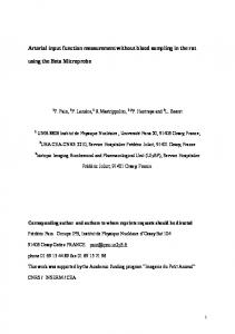
Of the 20 randomly selected patients, 19 had observable perfusion abnormalities; abnormalities in seven of these 19 patients were caused by vascular occlusions. The location of the automated AIF voxel was found to cover, or was located immediately adjacent to, a major vessel in each case: In 10 patients, the automated AIF voxel was located in the middle cerebral arterial branch in the sylvian fissure; in six patients, in the anterior cerebral artery in the interhemispheric fissure; in two patients, in the posterior cerebral artery within the deep calcarine fissure; and in two patients, in the basilar artery. In each case, the location suggested the presence of a vessel that had a predominantly inferosuperior course within the voxel. A single section that contained the voxel chosen as the AIF from each of the examinations in 20 patients is shown in Figure 2. The locations of the chosen voxels are shown as a small cross in each section. Quantitative Comparison: Automated AIF versus User-defined AIF In all 20 cases both the automated and user-defined AIFs were successfully fit to a gamma-variate function. Visual inspection of the ⌬R2* fit confirmed that the automated AIF exhibited the characteristic gamma-variate shape. The peak ⌬R2*, the FWHM, and the CBVratio for the two AIFs are included in the Table. The mean differences between the automated and user-defined AIF were ⫺0.16 sec⫺1 ⫾ 0.99 and 14.87 sec ⫾ 20.66, respectively, for the FWHM and peak ⌬R2* distributions. The peak ⌬R2* was significantly higher
(P ⬍ .05) with the automated AIF (⌬R2* ⫽ 46.35 sec⫺1 ⫾ 14.80) than it was with the user-defined AIF (⌬R2* ⫽ 31.48 sec⫺1 ⫾ 10.78). The CBVratio significantly exceeded 1.0 (CBVratio ⫽ 1.97 ⫾ 2.53; P ⬍ .05). The FWHM was smaller for the automated AIF (FWHM ⫽ 2.47 sec ⫾ 0.68) than it was for the user-defined AIF (FWHM ⫽ 2.63 sec ⫾ 1.01); however, these differences were not statistically significant (P ⫽ .67).
Discussion Findings of this study indicate that perfusion-weighted MR images can be generated reliably with a program that automatically identifies the AIF. Requiring no operator input, this method allows rapid, standardized calculation of relative CBF without the need for off-line image processing. The automated AIF had a greater peak value and a smaller width at half maximum, which suggests less partial-volume averaging artifact than that with the user-defined AIF. The CBVratio calculated on the basis of the automated AIF is significantly greater than that calculated with the user-defined AIF. Since the program selects the AIF on the basis of its time course rather than on the basis of anatomic location, operator selection bias is eliminated and partial-volume averaging is minimized. The automated AIF algorithm can be used to eliminate off-line postprocessing of dynamic susceptibility contrast MR images and the need for specially trained personnel. The automation of the determination of an AIF could potentially remove several steps in the processing of dynamic susceptibility contrast MR images. Streamlining the generation of relative CBF images may prove beneficial for time-critical applications, such as the delineation of ischemic regions in patients who have acute stroke. Elimination of the complexity in image processing could potentially result in broader dissemination of the dynamic susceptibility contrast MR imaging technology in the radiology community. In this pilot study of the reliability of the automated AIF, perfusion images were successfully produced with no additional off-line postprocessing and were reviewed as part of the nominal patient work-up. The automated AIF curves had a more “arterial” shape than the user-defined AIF curves, in the sense that they were less broadened, as might occur as the bolus of contrast material passes through the vascular bed. Although AIFs
Arterial Input Function for Assessment of Cerebral Blood Flow
䡠
595
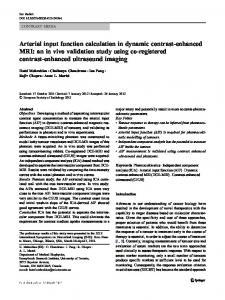
Radiology Figure 1. Images obtained in a 64-year-old woman with acute stroke and perfusion-diffusion mismatch. The patient had sudden onset of right hemiparesis and aphasia (National Institutes of Health Stroke Scale score, 20). A, Transverse intermediate-weighted image obtained at 3 hours 10 minutes after onset shows no parenchymal signal intensity changes. There is no evidence of arterial flow seen beyond the proximal left middle cerebral artery on the intermediate-weighted image. B, Three-dimensional time-of-flight image with no arterial flow seen. C, Transverse diffusion-weighted MR images (b ⫽ 1,000 sec/mm2) with an area of hyperintensity that correlated with the ischemic insult (arrow). D, Apparent diffusion coefficient maps with a region of reduced diffusion. Perfusion parameter maps were calculated by using the AIF method (Figure 1 continues).
calculated with the conventional method are not considered a reference standard, the conventional method represents a reasonable check on the accuracy of the automated method. The automated AIF is a robust means of generating parametric images of relative CBF, relative CBV, and MTT by using dynamic susceptibility contrast MR imaging. It routinely provides technically adequate images in clinical cases and, in particular, in those characterized by severe cerebrovascular disease. One potential criticism of the automated AIF is that it selects one and only one voxel that is used to deconvolve the entire data set. Classic tracer kinetic modeling assumes each capillary bed is supplied by a unique and different input function. Therefore, some groups have suggested that individual AIFs should be 596
䡠
Radiology
䡠
May 2003
applied to normal and ischemic territories. However, in clinical practice, the perfusion maps are used to identify areas that deviate from normal. Use of the single best internal “control” AIF, therefore, could be viewed as a practical advantage over the use of many individual AIFs, which would actually reduce sensitivity for low-flow lesions. No failures due to patient motion were identified in the pilot series, but the effect of patient motion on the reliability of the program has not been evaluated. The effect of congestive heart failure, arteriovenous shunting, or other conditions that might affect the automated program were also not systematically evaluated in this study. The AIF selected by the automated program appeared to localize on or immediately adjacent to a major artery. The pro-
gram selects the voxel on the basis of a large signal intensity change. A voxel containing an artery with an inferosuperior orientation was most likely chosen by the program, since such an anatomic relationship minimizes partial-volume averaging artifacts. Further processing of this AIF by using iterative techniques may be necessary for quantitative flow in milliliters per 100 g per minute (13). The program rejects veins because of the requirement that voxels selected have the earliest signal intensity changes. Venous structures such as the sagittal sinus appear to be effectively removed from the set of voxels considered as an AIF, and such locations were never chosen for the AIF in the cases analyzed. The AIF program also effectively discriminated signal intensity changes related to bolus passage from physiologic Carroll et al
Radiology
Figure 1 (continued). E, Map shows markedly prolonged MTT as normal to decreased. F, Map shows CBV. G, Map shows a severe overall reduction in CBF throughout the entire left middle cerebral artery territory. Parameter maps reconstructed off line (H, I) show similar patterns. H, Map shows voxels with prolonged transit time displayed in red, with the most rapid transit times shown in green. This image shows mean time to enhancement. I, Map shows relative CBV. Elevated relative CBVs are shown in red and lower values are shown in blue.
or imager noise unrelated to the passage of the bolus of contrast agent. In all 20 cases, a voxel with a characteristic gamma-variate shape was identified, which indicated that the chosen voxels were not anomalous noise spikes or other spurious signal changes. By using the proposed method of determining AIF, the potentially confounding effect of transient signal changes due to noise were minimized with integration of the signal intensity changes over several seconds. Selection of the AIF on the basis of minimum width or peak signal change would not likely have produced as reliable a result because of spurious brief fluctuations. An additional benefit of the signal Volume 227
䡠
Number 2
integration is that it correlates well with the determination of relative CBV (ie, rCBV), which may be calculated as follows: rCBV ⫽
冕
冕
关Gd兴共t兲dt/
AIF共t兲dt.
In this respect, we have chosen a voxel that has optimal relative CBV and therefore minimal partial-volume averaging. The reduced partial-volume averaging is evidenced by the fact that the automated AIF has both the higher peak ⌬R2* and the greater integrated contrast than the user-AIF. These results indicate less partial-volume averaging in the automated
AIF, which indicates a cleaner measure of the true AIF and, hypothetically, a more accurate determination of flow. The use of the arrival time parameter could potentially be modified and used to identify the time courses of venous efflux voxels. The identification of a venous time course has been shown to be useful in correction of AIF for quantitative determination of CBF (14). The use of this approach to automated quantitative CBF would present some advantages relative to previously reported quantitative CBF measures for which fewer sections were acquired and for which a dedicated imaging section was required to interrogate the distal carotid artery (8).
Arterial Input Function for Assessment of Cerebral Blood Flow
䡠
597
Radiology Figure 2. Cerebral blood flow images obtained in 20 randomly chosen patients (numbers in parentheses are patient numbers). The voxel that was identified as the automated AIF was demarked with a small cross (⫹) that was drawn by the postprocessing software to cover the chosen voxel. Two neuroradiologists identified the vascular anatomy of the AIF voxel. In all cases, the AIF was identified with an arterial branch, such as the middle cerebral artery, the anterior communicating artery, or the posterior communicating artery. Examples of these arteries are indicated with arrows.
However, in the current investigation, we do not have direct correlative studies with a reference standard. This is a limitation that prevents an evaluation of absolute CBF and the evaluation of the potential improvements afforded by the proposed venous efflux correction. The automated AIF algorithm, as in the case of the manual method, chooses a single voxel or region of interest to represent the AIF for the whole brain. There is some question as to whether the same AIF is appropriate to deconvolve tissue curves measured in a more proximal section. On the basis of simulations, Ostergaard et al (5) concluded that singular valued deconvolution underestimates flow measured from tissue curves that possess an arrival time delay relative to 598
䡠
Radiology
䡠
May 2003
the AIF. To validate this finding, Wirestam et al (7) compared AIFs recorded in the carotid artery with an AIF manually chosen in a proximal area of the imaging section. They were unable to reproduce the expectations of the simulations and found no difference in absolute cerebral perfusion when these two AIFs were compared. It should also be noted that on the basis of the original work of Ostergaard et al (5), Fourier deconvolution of an AIF will not exhibit the same sensitivity to arrival time. In short, the arrival time issue is one of the chosen deconvolution techniques and not the manner in which the AIF is chosen. The automated method has limitations. The algorithm depends on six parameters chosen for our specific imaging
protocol. The suitability of the algorithm for other protocols in which fewer precontrast points are obtained or smaller amounts of contrast medium are used has not been tested. However, with a suitable choice of parameters, it is anticipated that this algorithm can be suitably adjusted to other acquisitions. For example, in spin-echo acquisitions, the transient signal changes associated with bolus passage are not as great as they are in the gradient-echo acquisitions presented in this work. Therefore, a different criterion for determining the time of departure from baseline may be required with spin-echo acquisitions. It should be noted that we have successfully applied the automated AIF with the current set of parameters to spin-echo acquisitions in a Carroll et al
Comparison of Automated AIF and User-defined AIF on the Basis of ⌬R2*, FWHM, and CBVratio in 20 Patients
Radiology
Peak ⌬R2* (sec⫺1) Subject
FWHM (sec)
Automated AIF
User-defined AIF
Automated AIF
User-defined AIF
CBVratio
46.56 93.68 41.28 43.20 42.26 70.28 26.25 49.44 59.63 51.52 36.95 48.24 45.18 29.81 40.98 35.28 35.68 42.10 41.07 47.58 46.35 14.80
36.27 15.47 30.89 27.43 41.10 37.11 30.21 32.69 16.29 35.10 44.42 17.89 42.24 21.15 28.16 28.13 39.90 57.89 18.58 28.73 31.48 10.78
2.08 2.20 1.80 2.52 3.92 2.00 2.04 2.56 2.28 2.96 1.52 2.12 1.88 2.68 4.00 2.12 3.00 3.40 2.00 2.28 2.47 0.68
2.40 2.50 3.64 2.96 3.28 2.88 2.56 1.96 5.24 3.24 0.96 2.24 1.56 2.20 4.36 1.92 1.32 2.72 2.72 2.00 2.63 1.01
1.10 12.56 0.64 1.29 1.26 1.30 0.68 1.96 1.52 1.28 1.30 2.55 1.28 1.67 1.28 1.34 2.05 0.92 1.63 1.89 1.98 2.53
1 2 3 4 5 6 7 8 9 10 11 12 13 14 15 16 17 18 19 20 Mean SD
Note.—The mean difference, SD, and P value for automated AIF at peak ⌬R2* were 14.87, 20.66, and less than .05, respectively, and at FWHM, they were ⫺0.16, 0.99, and .67 (not significant), respectively. The P value for CBVratio was less than .05. All comparisons were determined with the Wilcoxon signed rank test.
Figure A1. Left: Adaptive threshold derived from the SD of signal intensity, , of a predetermined set of time frames (double arrows) was used to determine the mean precontrast signal intensity, S0. The averaged whole-brain signal intensity is used to determine the leading edge of the bolus of contrast agent on the basis of adaptive thresholds calculated from S0 and . The global arrival time is used to reject large signal changes associated with veins in the subsequent steps of the automated AIF calculation. Right: Second adaptive threshold was used to determine the arrival time of the leading edge of the bolus of contrast agent (arrows) on a voxel-by-voxel basis. The integrated signal depletion, , measured in units of (x,y,z), and arrival time determine the voxel that most accurately represents the AIF. The recirculation peak of the voxel chosen as the AIF voxel is used to remove the effects of recirculation on subsequent calculation of relative CBF, relative CBV, and MTT.
limited number of cases; however, a study in a larger number of patients is needed to establish its utility for these acquisitions. Finally, a more direct optimization of the relative CBV may be possible through the use of the ⌬R2* curve as opposed to the raw signal changes. In conclusion, we have evaluated an Volume 227
䡠
Number 2
automated rapid method of estimating AIF for the calculation of relative CBF at dynamic susceptibility contrast MR imaging. The automated AIF was found to yield relative CBF parametric images of diagnostic quality in 100 consecutive patients by using a standard MR imager and single-dose gadolinium-based contrast
material. In a randomly chosen sample of 20 patients, the voxel that was chosen as the AIF was found to be associated with signal changes in the middle, posterior, or anterior cerebral artery in or other arterial structures. When compared with the user-defined AIF, the automated AIF was found to have significantly higher peak ⌬R2* and similar bolus width as a user-defined AIF.
APPENDIX The automated AIF algorithm proposed in this work interrogates the sample of all voxels in the entire perfusion time-series to identify the voxel that optimally represents the AIF. The AIF voxel is optimized with respect to integrated signal change, which correlates with optimal blood volume. Voxels occupied by veins, and thus exhibit large CBV, are rejected with determination of their arrival time relative to other voxels. The automated AIF algorithm determines bolus arrival times on the basis of adaptive thresholds: thresholds for the arrival of contrast material and signal enhancement are measured in units of the SD of the precontrast signal. In this way, signal fluctuations from both physiologic and hardware noise that vary from image to image and patient to patient are implicitly included in the algorithm. Our algorithm can be delineated in five steps: (a) determine precontrast time frames, (b) calculate the contrast material arrival time of each voxel, (c) remove venous voxels on the basis of late contrast material arrival time, (d) find the arterial voxel with the highest peak signal change associated with bolus passage, and (e) determine the time limits of the bolus passage for the AIF deconvolution. These are described next. The precontrast time frames that are used for baseline signal and noise calculations are determined with the whole-brain signal intensity as a function of time. By using these average signal intensities, we estimate the mean precontrast signal and the SD by using frames acquired from 10 to 20 seconds after initiation of imaging. The 10 –20second time window is appropriate because our imaging protocol requires intravenous injection of contrast material 13 seconds after initiation of imaging to ensure contrast-free time frames for the determination of baseline signal intensity. The SD was used to determine an upper limit for signal fluctuation to determine precontrast frames (⬍3) and a threshold for contrast material arrival (⬎10), as shown in Figure A1. By using the precontrast frames determined from the analysis of the whole brain, the mean precontrast signal intensity, or S0 of each individual voxel located at position
Arterial Input Function for Assessment of Cerebral Blood Flow
䡠
599
Radiology
x,y,z and the SD, or (x,y,z), of each individual voxel were calculated and used to determine contrast material arrival time of each voxel. Since the changes of whole-brain signal versus time were dominated by signal in the large blood vessels, we calculated a separate arrival time threshold to determine voxel-by-voxel arrival time. The contrast material arrival time in each voxel is the first time point with a signal depletion of greater than 5 䡠 (x,y,z). This arrival time was used to identify any voxels with delayed arrival times. If the arrival time of a voxel was more than 2 seconds after the whole-brain arrival time, it was assumed to reflect flow in large venous structures and, therefore, was removed from further consideration as the AIF voxel. The AIF is defined as the voxel, of the remaining voxels, that exhibits the largest change in signal intensity sustained over four time frames, or roughly 8 seconds, in the current imaging protocol (Fig A1). The AIF was then used to determine the arrival of the contrast material and the recirculation peak of the bolus. This is accomplished with identification of the first time point after peak signal where the derivative of the AIF decreased to less than zero. The arrival time and recirculation points were used to determine the time limits for gamma-variate fits and the deconvolution of tissue concentration curves.
600
䡠
Radiology
䡠
May 2003
Acknowledgment: The authors acknowledge the contributions of Lindsey Nelson, BS. 8. References 1. Rosen BR, Belliveau JW, Vevea JM, et al. Perfusion imaging with NMR contrast agents. Magn Reson Med 1990; 14:249 – 265. 2. Rosen RR, Belliveau JW, Buchbinder BR, et al. Contrast agents and cerebral hemodynamics. Magn Reson Med 1991; 19:285–292. 3. Rosen RR, Belliveau JW, Aronen HJ, et al. Susceptibility contrast imaging of cerebral blood volume: human experience. Magn Reson Med 1991; 22:293–299. 4. Sunshine JL, Bambakidis N, Tarr RW, et al. Benefits of perfusion MR imaging relative to diffusion MR imaging in the diagnosis and treatment of hyperacute stroke. AJNR Am J Neuroradiol 2001; 22: 915–921. 5. Ostergaard L, Weisskoff RM, Chesler DA, et al. High resolution measurement of cerebral blood flow using intravascular tracer bolus passages. I. Mathematical approach and statistical analysis. Magn Reson Med 1996; 36:715–725 6. Ostergaard L, Sorenson AG, Kwong KK, et al. High resolution measurement of cerebral blood flow using intravascular tracer bolus passages. II. Experimental comparison and preliminary results. Magn Reson Med 1996; 36:726 –736. 7. Wirestam R, Andersson L, Ostergaard L, et al. Assessment of regional cerebral blood flow by dynamic susceptibility contrast MRA using different deconvolution tech-
9.
10. 11.
12.
13.
14.
niques. Magn Reson Med 2000; 43:691– 700. Rempp KA, Brix G, Wenz F, Becker CR, Gueckel F, Lorenz WJ. Quantification of regional cerebral blood flow and volume with dynamic susceptibility contrast-enhanced MR imaging. Radiology 1994; 193:637– 641. Carroll TJ, Rowley HA. Automatic determination of the arterial input function (AIF) in dynamic contrast-enhanced MRI in acute stroke (abstr). In: Proceedings of the Ninth Meeting of the International Society for Magnetic Resonance in Medicine. Berkeley, Calif: International Society for Magnetic Resonance in Medicine, 2001; 1578. Zierler KL. Equations for measuring blood flow by external monitoring of radioisotopes. Circ Res 1965; 16:309 –321. Sorenson AG, Copen WA, Ostergaard L, et al. Hyperacute stroke: simultaneous measurement of relative cerebral blood volume, relative cerebral blood flow and mean tissue transit time. Radiology 1999; 210:519 –527. Press WH, Teukolsky SA, Vetterling WT, Flannery BP. Numerical recipes in C. 2nd ed. Cambridge, England: Cambridge University Press, 1992. Van Osch MJP, Vonken EJPA, Bakker CJG, Viergever MA. Correcting partial volume artifacts of the arterial input function in quantitative cerebral perfusion MRI. Magn Reson Med 2001; 45:477– 485. Lin W, Celik A, Derdeyn C, et al. Quantitative measurement of cerebral blood flow in patients with unilateral carotid artery occlusion: a PET and MR study. J Magn Reson Imaging 2001; 14:659 – 667.
Carroll et al