Automatic Generation of Neural Networks based on Genetic Algorithms Fiszelew, A.1, Britos, P. 2, 3, Perichisky, G. 3 & García-Martínez, R. 2 1
Intelligent Systems Laboratory. School of Engineering. University of Buenos Aires. Paseo Colón 850 4to Piso. Ala Sur. (1063). Capital Federal. ARGENTINA
[email protected] 2 Software & Knowlwdge Engineering Center (CAPIS). Buenos Aires Institute of Technology. Av. Madero 399. (1106) Capital Federal. ARGENTINA
[email protected],
[email protected] 3 Ph.D. Computer Science Program. School of Computer Science. National University of La Plata. ARGENTINA
[email protected] Abstract - This work deals with methods for finding optimal neural network architectures to learn particular problems. A genetic algorithm is used to discover suitable domain specific architectures; this evolutionary algorithm applies direct codification and uses the error from the trained network as a performance measure to guide the evolution. The network training is accomplished by the backpropagation algorithm; techniques such as training repetition, early stopping and complex regulation are employed to improve the evolutionary process results. The evaluation criteria are based on learning skills and classification accuracy of generated architectures Key-words: evolutionary computation, neural networks, genetic algorithms, codification methods. Introduction The artificial neural networks offer an attractive paradigm for the design and the analysis of adaptive intelligent systems for a wide range of applications in artificial intelligence [1, 2]. Despite the great activity and investigation in this area during last years, that led to the discovery of relevant theoretical and empirical results, the design of neural networks for specific applications under certain designing constrains (for instance, technology) is still a test and error process, depending mainly on previous experience in similar applications [3]. The performance (and cost) of a neural network for particular problems is critically dependant on, among others, the choice of the processing elements (neurons), the net architecture and the learning algorithm [4, 5, 6, 7, 8, 9]. This work is focused in the development of methods for the evolutionary design of architectures for artificial neural networks. Neural networks are usually seen as a method to implement complex non-linear mappings (functions) using simple elementary units
interrelated through connections with adaptive weights [10, 11]. We focus in optimizing the structure of connectivity for these networks. Evolutionary design of neural architectures The key process in the evolutionary approach for topology designing is depicted in figure 1.
Figure 1 Design process of evolutionary neural architectures In the most general case, a genotype can be thought as an array of genes, where every gene takes a value from a properly defined domain [12]. Each genotype codes a phenotype or candidate
1
solution for the domain of interest – in our case a neural architecture class. Such codifications could use genes that take numeric values to represent a few parameters or complex structures of symbols that become into phenotypes (in this case neural networks) by means of a proper decodification process. This process can be extremely simple or quite complex. The resulting neural networks (the phenotypes) can also be equipped with learning algorithms that train them using stimulus from the environment or simply be evaluated in a given task (assuming that the weights of the net are also settled by the coding / decoding mechanism). This evaluation of a phenotype determines the fitness of its corresponding genotype [13, 14]. The evolutionary procedure works in a population of such genotypes, preferably selecting genotypes that code phenotypes with a high fitness, and reproducing them. Genetic operators such as mutation, crossover, etc., are used to introduce variety into the population and to test variants of candidate solutions represented in the current population. In this way, over several generations, the population gradually will evolve toward genotypes that correspond to phenotypes with high fitness.
particular, like we mention previously, it is possible that the network ends up overfitting the training data if the training session is not stopped at the right time. We can identify the beginning of overfitting by using crossed validation: the training examples are split into an training subset and a validation subset. The training subset is used to train the network in the usual way, except for a little modification: the training session is periodically stopped (every a certain number of epochs), and the network is evaluated with the validation set after each training period. The figure 2 shows the conceptualized forms of two learning curves, one belonging to measures over the training subset and the other over the validation subset. Usually, the model doesn't work so well on the validation subset as it does on the training subset, the design of which the model was based on. The estimation learning curve decreases monotonously to a minimum for a growing number of epochs in the usual way. In contrast, the validation learning curve decreases to a minimum, then it begins to increase while the training continues.
The generalization problem
When we look at the estimation learning curve it seems that we could improve if we go beyond the minimum point on the validation learning curve. In fact, what the network is learning beyond that point is essentially noise contained in the training set. The early stopping heuristic suggests that the minimum point on the validation learning curve should be used as an approach to stop the training session.
The topology of a network, that is, the number of nodes and the location and the number of connections among them, has a significant impact in the performance of the network and its generalization skills. The connections density in a neural network determines its ability to store information. If a network doesn't have enough connections among nodes, the training algorithm may never converge; the neural network will not be able to approximate the function. On the other hand, overfitting can happen in a densely connected network. Overfitting is a problem of statistical models where too many parameters are presented. This is a bad situation because instead of learning how to approximate the function presented in the data, the network could simply memorize every training example. The noise in the training data is then memorized as part of the function, often destroying the skills of the network to generalize.
Figure 2 Representation of the early stopping heuristic based on crossed validation.
Having good generalization as a goal, it is very difficult to realize the best moment to stop the training if we are looking only at the training learning curve. In
The question that arises here is how many times we should let the training subset not improve over the validation subset, before stopping the training ses-
In this work, the genotype only codes the architecture of a neural network with forward connections. The training of the weights for those connections is carried out by the back-propagation algorithm.
2
sion. We define an early-stopping parameter β to represent this number of training epochs.
(a) 0010 0000 0100 1010 0011 0111
The permutation problem
(b)
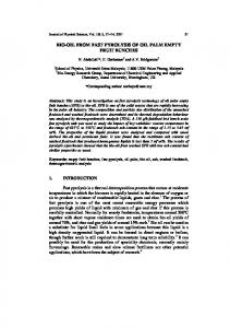
A problem that evolutionary neural networks face is the permutation problem. It not only makes evolution less efficient, but also hinders to the recombination operators the production of children with high fitness. The reason is the many-to-one mapping from the coded representation of a neural network to the real neural network decoded, because two networks that order their hidden nodes in different ways have different representation but can be functionally equivalent, as shown in the figures 3 and 4.
Figure 4 (a) A neural network that is equivalent to the one in figure 3(a); (b) The representation of the genotype under the same scheme of representation. To attenuate the effects of the permutation problem, we implement a phenotype crossover, that is, a crossover that works on neural networks rather than on chains of genes that make up the population. Another operator that helps in the face of the permutation problem is mutation. This operator induces to explore the whole search space and allows maintaining a genetic diversity in the population, so that the genetic algorithm is able to find solutions among all the possible permutations of the network. The noisy fitness evaluation problem The evaluation of the fitness of the architectures of neural networks will always be noisy if the evolution of the architectures is separated from the training of the weights. The evaluation is noisy because what is used to evaluate the fitness of the phenotype is the real architecture with weights (that is, the phenotype created from the genotype) and the mapping between phenotype and genotype is not one-to-one.
(a) 0100 1010 0010 0000 0111 0011 (b) Figure 3 (a) A neural network with its connection weights; (b) A binary representation of the weights, assuming that each weight is represented with 4 bits. Zero jeans no connection.
Such a noise can deceive to evolution, because the fact that the fitness of a phenotype generated from genotype G1 is higher than the fitness of a phenotype generated from genotype G2 doesn't imply that G1 has truly better quality that G2. To reduce this noise, we train each architecture many times starting from different initial weights chosen randomly. Then we take the best result to estimate the fitness of the phenotype. This method increases the computation time for the fitness evaluation, so a compromise must be achieved among the attenuation of the noise and the number of repetitions for the training. The complexity-regularization problem As the network design is statistical in nature, we need an appropriate tradeoff between reliability of the training data and goodness of the model. In the context of back-propagation learning, we may realize this tradeoff by minimizing the total risk expressed as: R(w) = εS(W) + λ εC(w)
3
The first term, εS(W), is the standard performance measure, which depends on both the network (model) and the input data. In back-propagation model learning it is typically defined as a meansquare error whose extends over the output neurons of the network and which is carried out for all the training examples on an epoch-by-epoch basis. The second term, εC(w), is the complexity penalty, which depends on the network (model) alone; its inclusion imposes on the solution prior knowledge that we may have on the models being considered. We can think of λ as a regularization parameter, which represent the relative importance of the complexity-penalty term with respect to the performance-measure term. In the weight-decay procedure that we used, the complexity penalty term is defined as the squared norm of the weight vector w (i.e., all the free parameters) in the network, as shown by:
ε C (w ) = w = 2
∑w
i∈Ctotal
2
i
where the set Ctotal refers to all the synaptic weights in the network. This procedure operates by forcing some of the synaptic weights to take values close to zero, while permitting others to retain their relatively large values. Accordingly, the weights of the network are grouped roughly into two categories: those that have a large influence on the network (model), and those that have little or no influence on it. The weights on the latter category are referred to as excess weights. In the absence of complexity regularization, these weights result in poor generalization by virtue of their high likelihood of taking on completely arbitrary values or causing the network to overfit the data in order to produce a slight reduction in the training error. The use of complexity regularization encourages the excess weights to assume values close to zero, and thereby improve generalization. Experimental design The hybrid algorithm that we employ for the automatic generation of neural networks uses a direct coding scheme, and develops the following steps: 1. Create an initial population of individuals (neural networks) with random topologies. Train each individual using the back-propagation algorithm. 2. Select the mother and the father from the population. 3. Recombinate both parents to obtain two
children. 4. Mutate each child randomly. 5. Train each child using propagation algorithm.
the
back-
6. Replace the children into the population. 7. Repeat from step 2 for a given number of generations. Parameters used in the Genetic Algorithm This algorithm applies a tournament selection (ordinal based) and replacement consists on a steady state update also implemented with a tournament technique. The tournament size is 3. A hundred of generations for the genetic algorithm are carried out in every experiment. All the experiments use a population size of 20. This is a standard value used in genetic algorithms. We make here a compromise among selective pressure and calculation time. The employment of 20 individuals is good to accelerate the development of the experiments without affecting at the results. Parameters used in the Neural Network Each neural network has 2 hidden layers and is trained over 500 epochs with back-propagation. This value is higher than the one usually used to train neural networks, giving enough time to the training to converge, and so taking advantage of the whole potential of each network. The back-propagation algorithm is based on the sequential training mode; the activation function chosen for each neuron is the hyperbolic tangent. We use a number of back-propagation repetitions equal to 3 to train each neural networks starting from different random initial weights. The best result is then used to estimate the fitness of the network. This algorithm provides an “approximation” to the trajectory in the weight space calculated by the descendant gradient method. The correction ∆wji(n) applied to the weight that connects the neuron i to the neuron j is defined by the delta rule:
A simple way to increment the learning rate and at the same time avoid the risk of instability (oscillations in the net) is to modify the delta rule including a momentum term, lie shown in:
4
∆w ji (n ) = α∆w ji (n − 1) + ηδ j (n)y i (n )
Some results from experimentation
where α is usually a positive number called the momentum constant. In the experimentation, the learning rate η is 0.1 and the momentum constant is 0.5. The database used The database chosen for the experimentation was taken form a file of datasets in Internet [15]. It consists on data concerning 600 applications for credit cards. Each application represents a sample for the training. The information of the application comprises the input for the neural network during the learning phase. The output is a true/false value that specifies whether the application was accepted or rejected. All the data in the applications is changed into meaningless symbols to protect the confidentiality. The attributes of a sample are similar to:
Figure 5 Complexity-regularization with adjustable regularization parameter: (1) λ=0 (no regularization); (2) λ=0.05; (3) λ=0.01; (4) λ=0.15
b,30.83,0,u,g,w,v,1.25,t,t,01,f,g,00202,0,+ In order to present the data to the network, the maximum and minimum values for every attribute into the training set are determined, then they are scaled between -1 and +1. The non-numerical inputs (multiple-choice) are treated in the same way, using discrete intervals. Using these methods of transformation, we obtain a 47 inputs network. The + sign at the end of the example stands for the class of the sample. In this case it will be a + or a -, depending on the approbation of the application, therefore the network has two outputs, one that activates when it is approved and the other when is rejected.
Figure 6 Comparison of the hit percentage of neural networks generated with different regularization parameters λ.
Cross Validation The cross validation is employed in the experimentation with the intention of getting better results. The cross validation consists on swapping the training set and the validation set, in the way that each one is used for the opposite purpose. This method assures that any tendency found in the results is, in fact, just tendency, and not causality. Thus, the database is randomly partitioned into two sets of equal size that are in turns used as training and validation subsets.
Figure 7 Early-stopping with adjustable stopping parameter: (1) No early stopping; (2) β=2; (3) β=5; (4) β=10.
5
Figure 8 Comparison of hit percentage of neural networks generated with different early-stopping parameters β. Comparison of a resulting neural network with other networks To determine if the evolutionary process is actually improving or not the neural networks concerning with their domain-specific topologies, we compare a resulting net generated by the hybrid algorithm with the best random topology (the one generated in the first generation of the genetic algorithm). These nets are also compared with a topology similar to the one obtained by the hybrid algorithm but 100% connected (or fully connected). We observe the effects of the three different topologies on the convergence of the neural networks while they are trained with a data partition, as depicted in the figure 9. Then we evaluate their classification skills on another data partition, as shown in the figure 10.
Figure 10 Comparison of hit percentage for different topology and connectivity.
From figure 9 we see that the neural network generated by the hybrid algorithm is able to learn better a new set of data than the other nets, including the one that implements its same topology but is fully connected. The network generated by the hybrid algorithm also has the best percentage for classifying examples not seen previously, as it is illustrated in figure 10. Conclusions The real world often has problems that cannot be solved successfully by a single basic technique; each technique has its pros and its cons. The concept of hybrid system in artificial intelligence consists on combining two approaches, in a way that their weaknesses are compensated and their strengths are boosted. The aim of this work is to create a way of generating topologies of neural networks that can easily learn and classify a certain class of data. To achieve this, a genetic algorithm is used to find the best topology that fulfills this task. When the process finishes, the result is a population of domain-specific networks, ready to take new data not seen previously. The analysis of the results of the experiments de monstrates that this implementation is able to create neural networks topologies that in general work better than random or fully connected topologies when they learn and classify new domain-specific data.
Figure 9 Ability to learning new data using: (1) Hybrid algorithm topology; (2) Best random topology; (3) Hybrid algorithm topology but 100% connected.
An aspect that should be examined more deeply is how the cost of a topology should be determined. In the current implementation, the cost is simply the training error of the neural network on a partition of the data set. The question that arises here is if this
6
is the best way to determine the fitness of a topology.
Genetic algorithms and simulated annealing ( pp. 116-128).
Another step to take would be to repeat the experiments for different data sets. Scalability is an important problem in neural networks implementations, therefore it would be interesting to see how the current implementation scales to bigger networks that contain thousands of inputs.
9. Honavar V. and L. Uhr. (1993) Generative Learning Structures and Processes for Generalized Connectionist Networks. Information Sciences, 70:75--108.
A last issue that should be explored is parallelization of the genetic algorithm, especially considering the huge processing times involved during the experimentation. By parallelizing the algorithm, it is possible to increment the population's size, reduce the computational cost and so to improve the performance of the AG. The parallel genetic algorithms or PGAs constitute a recent area of investigation, and very interesting approaches exist such as the Coarse Grained (islands model) PGAs or the Fine Grain PGAs [16]. References 1. Hinton G. E. (1989) Connectionist Learning Procedures. Artificial Intelligence, vol. 40, pp. 185-234 2. Hertz J., A. Krogh and R. Palmer (1991) Introduction to the Theory of Neural Computation. Reading, MA: Addison-Wesley. 3. Dow R. J. and Sietsma J. (1991) Creating Artificial Neural Networks that generalize. Neural Networks, vol. 4, no. 1, pp. 198-209.
10. Yao Xin (1999) Evolving Artificial Neural Networks. School of Computer Science. The University of Birmingham. B15 2TT. 11. Yao X. and Liu Y. (1998) Toward Designing Artificial Neural Networks by Evolution. Applied Mathematics and Computation, 91(1): 83-90. 12. Goldberg D. E. (1991) A comparative analysis of selection schemes used in genetic algorithms. In Gregory Rawlins, editor. Foundations of Genetic Algorithms, pages 69-93, San Mateo, CA: Morgan Kaufmann Publishers. 13. Rich E. and Knight K. (1991) Introduction to Artificial Networks. MacGraw-Hill Publications. 14. Stone M. (1974) Cross-validatory choice and assessment of statistical predictions. Journal of the Royal Statistical Society, vol. B36, pp. 111133. 15. Blake C. L. y Merz C. J. (1998) UCI Repository of machine learning databases. http://www.ics.uci.edu/~mlearn/MLRepository.ht ml Irvine, CA: University of California, Department of Information and Computer Science. 16. Hue Xavier (1997) Genetic Algorithms for Optimization. Edinburgh Parallel Computing Centre. The University of Edinburgh.
4. Haykin Simon (1999) Neural Networks. A Comprehensive Foundation. Second Edition. Pretince Hall. 5. Holland J. H. (1975) Adaptation in Natural and Artificial Systems. University of Michigan Press (Ann Arbor). 6. Holland, J. H. (1980) Adaptive algorithms for discovering and using general patterns in growing knowledge-based. International Journal of Policy Analysis and Information Systems, 4(3), 245-268. 7. Holland, J. H. (1986) Escaping brittleness: The possibilities of general purpose learning algorithms applied in parallel rule-based systems. In R. S. Michaiski, J. G. Carbonell, & T. M. Mitchell (Eds. ), Machine Learning II (pp. 593-623). Los Altos, CA: Morgan Kaufmann. 8. Holland, J. H., Holyoak, K. J., Nisbett, R. E., & Thagard, P. R. (1987). Classifier systems, Qmorphisms, and induction. In L. Davis (Ed.),
7